3
Thermomechanical Effects in Liquid Crystals
Patrick OSWALD1, Alain DEQUIDT2 and Guilhem POY1
1Laboratoire de Physique, ENS de Lyon, France
2CNRS, SIGMA Clermont, Clermont Auvergne University, Clermont-Ferrand, France
3.1. Introduction
Any unconstrained thermodynamical system tends to spontaneously evolve in such a way as to homogenize its intensive variables.
Let us take a concrete example. In a conducting fluid containing a solute, for instance, these variables are the temperature, the pressure, the velocity, the chemical potential of the solute and the electric potential. The thermodynamic equilibrium state of this system is reached when all these variables are constant and the free energy is minimal. However, these variables vary in space and time during the equilibration phase. Thus, a non-homogeneous distribution of temperature will result in the appearance of a heat flux. Similarly, a gradient of chemical potential will produce a flux of solute, while a gradient of electric potential and/or velocity will generate an electric current and/or a flux of momentum.
To each of these irreversible phenomena is associated a transport coefficient, which enters into a transport law of the type
where Jk is the flux of the property k, γk is the associated transport coefficient and Xk is the gradient force that acts on this property.
In the previous example, these laws were known for a long time and correspond to the Fourier law (1822) for the heat flux, to the Fick law (1855) for the solute diffusion, to the Ohm law (1827) for the electric current and to the Newton law of viscosity (1687) for the velocity when the fluid is Newtonian. The associated transport coefficients are the thermal conductivity, the chemical diffusion coefficient, the electric conductivity and the dynamical viscosity.
Historically, these phenomenological laws were obtained empirically. However, it is possible to recover them by using the thermodynamics of irreversible phenomena (Prigogine 1967). This theory applies when the local equilibrium hypothesis is valid and supposes that there exist linear relations between the fluxes and the forces responsible for the transport phenomena. These general linear relations are important because they directly show that the transport phenomena can interfere with each other. This leads to crossed phenomena that are often smaller – and thus more difficult to measure – than the direct effects described above. For example, a temperature gradient may cause a concentration gradient (Soret effect or thermodiffusion) while a flux of heat can be generated by a difference in electric potential (a thermoelectric effect known as the Peltier effect). Inverse effects also exist, known as the Dufour effect in the chemical case and the Seebeck effect in the electric case. Many other effects of this type have been described in the literature such as the fountain effect in superfluid helium II. In that case, a temperature gradient inside a tube containing the superfluid generates a pressure gradient responsible for the expulsion of the superfluid out of the tube. Other examples, including electromagnetic and acoustical processes, are given in the reference book by de Groot and Mazur (1962).
In this chapter, we describe two crossed effects observed in nematic and cholesteric liquid crystals (LC) subjected to a temperature gradient ![]() . The first effect couples the rotation of the molecules to the temperature gradient (thermomechanical [TM] effect), while the second one couples the flows to the temperature gradient (thermohydrodynamical [TH] effect).
. The first effect couples the rotation of the molecules to the temperature gradient (thermomechanical [TM] effect), while the second one couples the flows to the temperature gradient (thermohydrodynamical [TH] effect).
These effects do not exist in usual fluids, but are possible in LCs because of the existence of a long-range orientational order of the molecules, to which is associated a new hydrodynamical variable, the director ![]() , which is the unit vector giving the mean orientation of the molecules at each point.
, which is the unit vector giving the mean orientation of the molecules at each point.
In practice, the director can experience a torque and rotate on itself in the absence of any flow. This irreversible process is dissipative and described by the phenomenological law
In this formula, of the same type as equation [3.1], ![]() is a viscous torque,
is a viscous torque, ![]() is the rotation rate of the director equal to
is the rotation rate of the director equal to ![]() in the absence of flow1 and γ1 is a transport coefficient known as the rotational viscosity. This effect is described by the vertical blue arrow on the right in the general scheme in Figure 3.1.
in the absence of flow1 and γ1 is a transport coefficient known as the rotational viscosity. This effect is described by the vertical blue arrow on the right in the general scheme in Figure 3.1.

Figure 3.1. Direct and crossed effects in nematic and cholesteric liquid crystals subjected to a temperature gradient. The thermomechanical effect is described by the red arrows in solid line and the thermohydrodynamical effect corresponds to the red dashed-line arrows. σ(s) is the symmetric part of the non-equilibrium stress tensor, D is the strain rate tensor,  is the heat flux,
  is the temperature gradient,
  is the non-equilibrium torque and
  is the director rotation rate
In nematic or cholesteric LCs, the Newton law for viscosity and the Fourier law for heat conduction can also be generalized for taking into account the particular symmetries of the phase. This leads to replace the viscosity and the thermal conductivity by a viscosity tensor νijkl and a thermal (or heat) conductivity tensor κij . In these systems, these two laws write in the form:
and
where ![]() is the symmetric part of the non-equilibrium stress tensor,
is the symmetric part of the non-equilibrium stress tensor, ![]() is the strain rate tensor (by denoting the derivative with respect to xj by a subscript j after a comma) and
is the strain rate tensor (by denoting the derivative with respect to xj by a subscript j after a comma) and ![]() is the heat flux. These two equations describe the two direct effects represented by the left and middle vertical blue arrows in Figure 3.1.
is the heat flux. These two equations describe the two direct effects represented by the left and middle vertical blue arrows in Figure 3.1.
Besides these direct effects, the thermodynamics of irreversible phenomena teaches us that crossed effects can also exist.
One of them is described by the green arrows in Figure 3.1. This crossed effect is well known in nematic and cholesteric LCs and couples the flows with the director rotation. This effect is described by another transport coefficient known as the rotational viscosity γ2 in the literature. This viscosity is very important and responsible in part for the “backflow” effects observed in numerous experiments (de Gennes and Prost 1995; Oswald and Pieranski 2005; Svenšek and Žumer 2001). The latter effect is even used in practice in, for instance, some bistable nematic LCD displays (Dozov et al. 1997).
In this chapter, we focus on the two other crossed effects represented in Figure 3.1. The first one is the TM effect represented by the solid line red arrows. It couples the director rotation to the temperature gradient. The second one is the TH effect represented by the dashed-line red arrows. It couples the flows to the temperature gradient.
These two effects were first predicted in undeformed cholesteric LCs by Leslie (1968) and later, independently, by Akopyan and Zel’dovich in 1984 and Brand and Pleiner in 1988 in deformed nematic LCs (Akopyan and Zel’dovich 1984; Brand and Pleiner 1988; Pleiner and Brand 1996). The general theory of these effects is given in Poy and Oswald (2018). In this paper, the calculations are extended to deformed cholesteric phases and the equivalence between the Akopyan and Zel’dovich model and the Brand and Pleiner model is demonstrated. We note right now that, for reasons to do with symmetry, these effects can only exist in systems that are not invariant under the reflection in a mirror. This is the case in the undeformed cholesteric phase of D2 symmetry2 in which no mirror symmetry exists because of the chirality of the phase, but not in the undeformed nematic phase of symmetry D∞h. In the nematic phase, TM and TH effects can only appear when the mirror symmetry of the director field is broken at the macroscopic level, i.e. when the phase is distorted. This is the reason why the transport coefficients ξij and ζijk describing these crossed effects in Figure 3.1 are reduced to two pure pseudoscalars (Leslie coefficients noted μ and ν in the following) in an undeformed cholesteric LC while the other coefficients – only present in deformed nematic or cholesteric phases – are linear functions of the director field distortions ni,j with proportionality coefficients that are pure scalars. We also emphasize that the cross-effect coefficients ξij and ζijk must satisfy the Onsager reciprocal relations (Onsager 1931a, 1931b; Wigner 1954) coming from the property of microscopic reversibility (Casimir 1945). These relations are respected in Figure 3.1 and we refer to Poy and Oswald (2018) for their demonstration. Finally, we recall that, according to the Curie principle, all the phenomenological equations must be invariant under the action of the symmetry group of the phase (D∞h for nematics, D∞ for cholesterics), undeformed or not, as explained in Poy and Oswald (2018).
The goal of this chapter is to review the main works, theoretical, numerical and experimental, on the TM and TH effects in nematic and cholesteric LCs. The rest of this chapter is divided in four sections. In section 3.2, we recall the basic equations of the nematodynamics and we give the general expressions of the constitutive equations in the presence of a temperature gradient. In section 3.3, we summarize the main theoretical results obtained by Sarman and coworkers by molecular dynamics simulations in the case of the TM effect. The last two sections are essentially experimental and deal, respectively, with the TM effect (section 3.4) and the TH effect (section 3.5). Several experiments will be described in these sections, in particular the Éber and Janossy experiment that revealed for the first time the existence of a TM effect in a cholesteric LC. Finally, conclusions and perspectives are drawn in section 3.6.
3.2. The Ericksen–Leslie equations
3.2.1. Conservation equations
In an ordinary fluid, the hydrodynamic variables are the density ρ, the velocity ![]() and the internal energy per unit volume e. In a nematic or a cholesteric LC, a new variable exists, the director
and the internal energy per unit volume e. In a nematic or a cholesteric LC, a new variable exists, the director ![]() . Each of these variables is associated with a conservation equation.
. Each of these variables is associated with a conservation equation.
The first one is the mass conservation equation, which reads in the incompressible limit
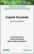
The next two equations derive from Newton’s second law. The first one describes the conservation of linear momentum. Also called Cauchy’s equation, it reads by neglecting body forces such as gravity:
In this equation, ![]() is the material derivative with respect to time,
is the material derivative with respect to time, ![]() has for components σij,j and σ ≡ −P
has for components σij,j and σ ≡ −P ![]() +σ(eq)+σ(neq) is the total stress tensor, which can be decomposed into a pressure term −P
+σ(eq)+σ(neq) is the total stress tensor, which can be decomposed into a pressure term −P ![]() (with
(with ![]() the identity matrix), an equilibrium elastic stress tensor σ(eq) and a non-equilibrium stress tensor σ(neq). The elastic stress tensor has for components
the identity matrix), an equilibrium elastic stress tensor σ(eq) and a non-equilibrium stress tensor σ(neq). The elastic stress tensor has for components ![]() by denoting by f the elastic energy of expression
by denoting by f the elastic energy of expression

Constants K1−4 are the usual Frank elastic constants and q0 is the equilibrium twist of the cholesteric phase (with q0 = 0 in the nematic phase and at the compensation temperature of the cholesteric phase, when it exists).
The second equation (torque equation) describes the conservation of angular momentum and is obtained by applying the angular momentum theorem. It reads
In this equation, ![]() is the non-equilibrium torque acting on the director and
is the non-equilibrium torque acting on the director and ![]() is the equilibrium elastic torque3 of expression
is the equilibrium elastic torque3 of expression ![]() where
where ![]() =
= ![]() is the molecular field of component
is the molecular field of component ![]() . Because the torques are perpendicular to
. Because the torques are perpendicular to ![]() we can set
we can set ![]() . With this notation, the torque equation rewrites under the equivalent form
. With this notation, the torque equation rewrites under the equivalent form
where ![]() represents the dyadic product between two vectors and (
represents the dyadic product between two vectors and (![]() −
− ![]() )
)![]() gives the component
gives the component ![]() of
of ![]() perpendicular to
perpendicular to ![]() .
.
The last equation is the heat equation. It comes from the energy conservation and reads by neglecting the term of thermal expansion
In this equation, A : B = AijBij represents the total contraction of the two second-order tensors A and B, Cp is the specific heat capacity at constant pressure, σ(s) is the symmetric part of σ(neq) and ![]() is the rotation vector of the director with
is the rotation vector of the director with ![]() the corotational time derivative of the director.
the corotational time derivative of the director.
Solving equations [3.5], [3.6], [3.8] (or [3.9]) and [3.10] with adequate boundary conditions gives the fields ![]() .
.
More precisely, we need to either know the velocity or the surface force at the boundary of the LC domain to solve the Cauchy equation. The latter condition reads
where ![]() is the unit vector normal to the boundary of the LC domain and directed outwards and
is the unit vector normal to the boundary of the LC domain and directed outwards and ![]() is the surface force imposed on the boundary.
is the surface force imposed on the boundary.
For the torque equation, the associated boundary condition reads
where γS is a surface viscosity, ![]() is the surface molecular field of components
is the surface molecular field of components ![]() by denoting by W(ni,T) the anchoring energy per unit surface area and C is the surface torque tensor of components
by denoting by W(ni,T) the anchoring energy per unit surface area and C is the surface torque tensor of components ![]() .
.
Finally, the temperature or the heat flux must be specified on the boundary of the LC domain to solve the heat equation.
In the next two sections, we give the complete expression of the bulk molecular field and we recall the constitutive equations compatible with the symmetries of the nematic or cholesteric phase.
3.2.2. Molecular field
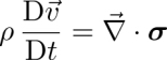
In static equilibrium, the torque equation [3.8] reduces to ![]() where
where ![]() is the molecular field and f is the elastic energy given in equation [3.7], which depends on four constants Ki(i = 1 − 4) describing, in order, the splay, twist, bend and splay-twist distortions. These constants usually depend on temperature, so that the molecular field contains terms proportional to Ki (this part will be denoted by
is the molecular field and f is the elastic energy given in equation [3.7], which depends on four constants Ki(i = 1 − 4) describing, in order, the splay, twist, bend and splay-twist distortions. These constants usually depend on temperature, so that the molecular field contains terms proportional to Ki (this part will be denoted by ![]() ) and terms proportional to
) and terms proportional to ![]() (static thermomechanical terms denoted by
(static thermomechanical terms denoted by ![]() ) when a temperature gradient is applied.
) when a temperature gradient is applied.
The former part is standard and reads in index form (Stewart 2004):
where ∊ijk is the Levi–Civita symbol and repeated indices are implicitly summed over. The reader will note that K4 does not enter into ![]() because the K4-contribution to the free energy appears as a surface-like term in div(...) when K4 is assumed to be constant.
because the K4-contribution to the free energy appears as a surface-like term in div(...) when K4 is assumed to be constant.
As for the static thermomechanical contributions coming from the temperature variation of the elastic constants, they read (Dequidt et al. 2016):

For completeness, we give the expressions of the magnetic and electric contribution to the free energy:

from which can be calculated the magnetic and electric contributions to the molecular field which add to ![]() when a magnetic field
when a magnetic field ![]() and/or an electric field
and/or an electric field ![]() are applied:
are applied:

Here, μ0 is the vacuum permeability, ε0 is the vacuum permittivity, χa is the magnetic anisotropy and εa is the dielectric anisotropy.
3.2.3. Constitutive equations
The constitutive equations are obtained by first calculating the irreversible entropy production. A straightforward calculation gives (de Gennes and Prost 1995; Oswald and Pieranski 2005)
In this expression, σ is the density of entropy, σ(s) is the symmetric part of the non-equilibrium stress tensor and ![]() is the entropy flux.
is the entropy flux.
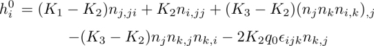
The next step consists of writing linear relations between forces and fluxes once they have been chosen. The details of these calculations and the complete expressions of tensors ![]() defined in Figure 3.1 by taking
defined in Figure 3.1 by taking ![]() and D as forces and
and D as forces and ![]() and σ(s) as fluxes, are given in Poy and Oswald (2018)4. From these expressions, the symmetric part of the non-equilibrium stress σ(s) and the non-equilibrium torque
and σ(s) as fluxes, are given in Poy and Oswald (2018)4. From these expressions, the symmetric part of the non-equilibrium stress σ(s) and the non-equilibrium torque ![]() can be calculated.
can be calculated.
Three contributions must be considered. The usual viscous contribution involving the Leslie viscosity coefficients αi(i = 1 − 6) (blue and green arrows in Figure 3.1), the Leslie contribution to the TM and TH effects (present in cholesterics only) and the Akopyan and Zel’dovich contributions to the TM and TH effects, which are linear in ![]() and appear in both deformed nematic and cholesteric LCs:
and appear in both deformed nematic and cholesteric LCs:
From these expressions, the complete non-equilibrium stress tensor can then be calculated by remembering that σ(neq) ≡ σ(s)+σ(a), where σ(a) is the antisymmetry part of this tensor coming from the non-equilibrium torques of components
where δij is the Knonecker delta.
In the following, we give the result of these calculations for each contribution.
3.2.3.1. Usual viscous terms
With the Leslie notations, the viscous force and the symmetric part of the viscous stress tensor reads:
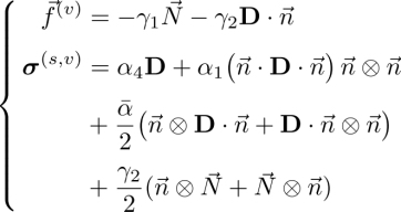
In this expression, the coefficients γ1, α1, α4 (which appears as an “ordinary” viscosity) and ![]() represent the direct effects represented by the blue left and right arrows in Figure 3.1, while γ2 describes the crossed effect represented by the green arrows in this figure.
represent the direct effects represented by the blue left and right arrows in Figure 3.1, while γ2 describes the crossed effect represented by the green arrows in this figure.
This gives the following well-known expression for the complete viscous stress tensor:

where ![]() From these relations, we calculate γ1 = α3 − α2 and γ2 = α2 + α3 with α2 + α3 = α6 − α5, an equality known as the Parodi relation (1970). This relation shows that the six viscosity coefficients αi, initially introduced by Leslie, are not independent because of the reciprocal Onsager relation that applies to the crossed effect “γ2”, represented by the green arrows in Figure 3.1. We underline that all the viscosities (including γ2) enter by construction into the expression of the complete viscous stress tensor.
From these relations, we calculate γ1 = α3 − α2 and γ2 = α2 + α3 with α2 + α3 = α6 − α5, an equality known as the Parodi relation (1970). This relation shows that the six viscosity coefficients αi, initially introduced by Leslie, are not independent because of the reciprocal Onsager relation that applies to the crossed effect “γ2”, represented by the green arrows in Figure 3.1. We underline that all the viscosities (including γ2) enter by construction into the expression of the complete viscous stress tensor.
3.2.3.2. Leslie TM and TH terms
These terms are only present in cholesterics in which no mirror symmetry exists because of the chirality of the phase. According to Leslie, these terms read (Leslie 1968):

Here, ν is the TM Leslie coefficient5 and μ is the TH Leslie coefficient. From the previous equations, the Leslie contribution to the total non-equilibrium stress tensor can be calculated:
with μ1 = (μ + ν)/2 and μ2 = (μ − ν)/2. As for the viscosities, we note that the two coefficients μ and ν enter into the expression of the total stress tensor, while only ν enters into the expression of the thermomechanical force. Another important point is to note that μ and ν (and thus μ1 and μ2) are pseudoscalars that must vanish in a nematic phase for symmetry reasons.
3.2.3.3. Akopyan and Zel’dovich TM and TH terms
These terms appear in both cholesteric and nematic LCs when the director field is distorted. These terms linear in ![]() are much more complicated. By using the Akopyan and Zel’dovich notations, they read:
are much more complicated. By using the Akopyan and Zel’dovich notations, they read:

where ![]() . In these equations, the coefficients
. In these equations, the coefficients ![]() are the thermomechanical Akopyan and Zel’dovich coefficients and the coefficients
are the thermomechanical Akopyan and Zel’dovich coefficients and the coefficients ![]() are the thermohydrodynamical coefficients.
are the thermohydrodynamical coefficients.
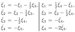
Actually, the four TM coefficients can be associated with the four fundamental deformations of the director field. This is not so readily apparent when one looks at the previous equation. For this reason, we proposed in Oswald et al. (2017) to rewrite this force in the equivalent form:

where we defined the splay, twist, bend and Gauss contributions to the thermomechanical effects as:
The correspondence between the new TM coefficients ![]() and the ξ1−4 of Akopyan and Zel’dovich is as follows:
and the ξ1−4 of Akopyan and Zel’dovich is as follows:
A similar procedure can also be applied to the eight TH coefficients ξ5−12 and leads to the equivalent form for σ(s,AZ):
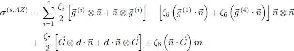
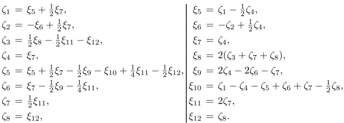
The correspondence between the new TH coefficients ζ1−8 and the ξ5−12 of Akopyan and Zel’dovich is as follows:
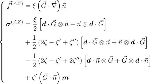
From the previous equations, the Akopyan and Zel’dovich contribution to the total non-equilibrium stress tensor and force can be obtained. Its general expression is very complex and will not be given here. A simplified expression can be found by assuming that the new TM coefficients are all equal ![]() and by setting ζ1−6 ≡ 2ζ − ζ′ + ζ″, ζ7 ≡ ζ′ − 2(ζ + ζ″) and ζ8 ≡ ζ′ for the new TH coefficients. With this choice, we find:
and by setting ζ1−6 ≡ 2ζ − ζ′ + ζ″, ζ7 ≡ ζ′ − 2(ζ + ζ″) and ζ8 ≡ ζ′ for the new TH coefficients. With this choice, we find:
The definitions of the coefficients ζ, ζ′ and ζ″ may feel a bit convoluted for now, but we will see later that, for some specific geometries, the terms in ζ′ and ζ″ do not contribute to the Navier–Stokes equation, thus motivating the convention adopted here. Again, we see that both TM and TH coefficients ξ1−12 enter into the expression of the total stress tensor, whereas only the TM coefficients ξ1−4 enter into the expression of the TM force. Last but not least, it is important to note that the ξi are true scalars, contrary to the Leslie coefficients μ and ν, which are pseudoscalars.
3.2.3.4. Heat conductivity tensor
The tensor of heat conductivity is given by
where ![]() is the transverse Kronecker delta. In this expression, κ⊥ and κ‖ are the thermal conductivities perpendicular and parallel to the director. To these usual terms add the TM and TH terms that are extremely small in comparison with the latter of the order of 10−12 − 10−11 in relative value (Dequidt et al. 2016). For this reason, they can be neglected and we shall not give them here. Their complete expression is however given in Poy and Oswald (2018).
is the transverse Kronecker delta. In this expression, κ⊥ and κ‖ are the thermal conductivities perpendicular and parallel to the director. To these usual terms add the TM and TH terms that are extremely small in comparison with the latter of the order of 10−12 − 10−11 in relative value (Dequidt et al. 2016). For this reason, they can be neglected and we shall not give them here. Their complete expression is however given in Poy and Oswald (2018).
3.3. Molecular dynamics simulations of the thermomechanical effect
The previous Leslie and Akopyan and Zel’dovich theories of the TM effect are purely phenomenological and cannot help to understand its molecular origin. To achieve this, molecular simulations are necessary. They have all been performed by Sten Sarman and his coworkers. The first studies date back to the late 1990s.
3.3.1. Molecular models
Although the efficiency of computers keeps on increasing, the molecular simulation of LCs with atomic resolution is still a challenge, especially when the goal is to compute transport coefficients. This is because:
- 1) the simulation of a liquid phase with long-range orientational order requires big systems with many molecules;
- 2) transport coefficients require long acquisition times, especially for viscous systems with slow relaxation like LCs.
For this reason, molecular simulations of LCs are rather performed using simpler coarse grain models (Wilson 2005, 2007). The coarse grains need to have anisotropic interactions in order to produce liquid crystalline phases. The most common coarse grain model for LCs is the Gay–Berne potential (Gay and Berne 1981). This model is generic and simulated using reduced units.
Sarman and co. generally used a simplified version of this potential, consisting only of a short-range repulsive interaction:

where ![]() is the orientation-dependent strength of the interaction, while
is the orientation-dependent strength of the interaction, while ![]() is the orientation-dependent diameter of the grain. σ0 is the diameter of the grain perpendicular to the grain axis
is the orientation-dependent diameter of the grain. σ0 is the diameter of the grain perpendicular to the grain axis ![]() . The grains described by this potential are rigid ellipsoids of revolution, which can be oblate or prolate (Figure 3.2). They form discotic or calamitic nematic phases in a given range of temperature and number density, depending on their aspect ratio. In order to form cholesteric phases, the interactions have to include a chiral component. The simulations of Sarman use two types of cholesteric models due to (Memmer et al. 1995; Memmer and Kuball 1996; Memmer 1998, 2000):
. The grains described by this potential are rigid ellipsoids of revolution, which can be oblate or prolate (Figure 3.2). They form discotic or calamitic nematic phases in a given range of temperature and number density, depending on their aspect ratio. In order to form cholesteric phases, the interactions have to include a chiral component. The simulations of Sarman use two types of cholesteric models due to (Memmer et al. 1995; Memmer and Kuball 1996; Memmer 1998, 2000):
- – The old simulations of the 2000s define molecules as rigid twisted strings of six oblate Gay–Berne ellipsoids (Sarman 2000, 2001) (see Figure 3.3). The long axis of the molecule is along the axis of the cholesteric helix, while the director is the average orientation of the small or intermediate axis of the molecules. This means that the phase is biaxial, with a strong nematic ordering of the long axes
 along the helical axis (order parameter S1 ∼ 0.8) and a weaker cholesteric ordering of the intermediate axes
  perpendicular to the helical axis (order parameter S2 ∼ 0.5). The director is defined here using the orientations of
  . This does not correspond to the usual cholesterics used in experiments.
 - – The newer simulations of the 2010s define molecules as single Gay–Berne ellipsoids plus a chiral potential (Sarman and Laaksonen 2013; Sarman et al. 2016):

where c is the strength of the chiral interaction. This model is closer to experimental cholesteric systems, with the director corresponding to the long axis of the ellipsoids.
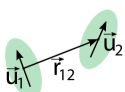
Figure 3.2. Gay–Berne ellipsoids illustrating the notations of equation [3.33]
3.3.2. Constrained ensembles
The simulations are performed under periodic boundary conditions, so as to mimic an infinite medium without border effects. The simulation box is a fixed cuboid. For the simulation of nematic systems, the director is uniform and aligned with one of the axes. For the simulation of cholesteric systems, the box size has to be a multiple of the cholesteric half pitch, often a full pitch. The match between the pitch and the box size is not obtained by varying the box size, but by varying the strength of the chiral interaction until the pressure becomes isotropic. This way, the cholesteric has its equilibrium twist. It should be noted that the small size of the simulation box limits the study to cholesterics of very small pitch and therefore systems that are much more chiral than those in the experiments (Sarman 2000).

Figure 3.3. Rigid twisted string of six oblate Gay–Berne ellipsoids featuring a cholesteric molecule in the older simulations
The eigenvector of the tensor order parameter Q associated with the greatest eigenvalue, where Q can be calculated directly from the grain axes ![]() :
:
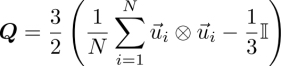
defines an effective director ![]() . In cholesteric systems, the average in the expression of Q is done after untwisting the helix by rotating the vectors
. In cholesteric systems, the average in the expression of Q is done after untwisting the helix by rotating the vectors ![]() by an angle −qzi around
by an angle −qzi around ![]() , the axis of the helix, q being its torsion. This allows us to define a single order parameter for the whole system, even in the cholesteric case (in this case it should be noted that
, the axis of the helix, q being its torsion. This allows us to define a single order parameter for the whole system, even in the cholesteric case (in this case it should be noted that ![]() does not represent the real director field of the cholesteric helix).
does not represent the real director field of the cholesteric helix).
In order to avoid the angular diffusion of the effective director, Sarman constrains its direction using Lagrange (or Gauss) multipliers, which represent an external torque applied to ![]() (Sarman and Evans 1993; Sarman 1996). The effective director
(Sarman and Evans 1993; Sarman 1996). The effective director ![]() is thereby held fixed, without any fluctuations. This method also allows us to impose a constant angular velocity of the director,
is thereby held fixed, without any fluctuations. This method also allows us to impose a constant angular velocity of the director, ![]() , or to impose a constant external torque
, or to impose a constant external torque ![]() on the director and to let it be free to rotate.
on the director and to let it be free to rotate.
The simulations are performed at constant temperature using the same kind of constraint, which corresponds to isokinetic simulations. This means that there are no temperature fluctuations.
Nevertheless, although the temperature T is constant and uniform, a fictitious heat field ![]() can be applied, which has the same effect as applying a temperature gradient (in fact
can be applied, which has the same effect as applying a temperature gradient (in fact ![]() By this mean, it is possible to study the effect of a temperature gradient, while T is actually uniform (Schlacken 1987; Evans and Murad 1989; Sarman and Evans 1993). The way it works is the following: The equations of motion are perturbed by adding external forces and torques proportional to
By this mean, it is possible to study the effect of a temperature gradient, while T is actually uniform (Schlacken 1987; Evans and Murad 1989; Sarman and Evans 1993). The way it works is the following: The equations of motion are perturbed by adding external forces and torques proportional to ![]() so that energy is dissipated. The additional terms are chosen in such a way that the conserved quantities (linear and angular momentum) are not perturbed and that the rate of dissipation per unit volume is
so that energy is dissipated. The additional terms are chosen in such a way that the conserved quantities (linear and angular momentum) are not perturbed and that the rate of dissipation per unit volume is ![]() , namely the same as in the presence of a temperature gradient
, namely the same as in the presence of a temperature gradient ![]() It was shown that, in these circumstances, the system responds in terms of thermodynamic fluxes as if it was subjected to a temperature gradient.
It was shown that, in these circumstances, the system responds in terms of thermodynamic fluxes as if it was subjected to a temperature gradient.
3.3.3. Computation of the transport coefficients
The simulations enable the computation of transport coefficients either from non-equilibrium simulations by imposing finite thermodynamic forces and measuring the thermodynamic fluxes, or from equilibrium simulations using the Green–Kubo formulas (Sarman 1999).
The former method was most often chosen in the older simulations, because it requires less long simulation runs and is more computationally affordable. However, it is usually necessary to drive the system quite far from equilibrium and possibly out of the linear regime in order to measure a significant response. Indeed, small systems are the place of big fluctuations, which may hide the thermodynamic fluxes. In addition, equilibrium simulations give access to all the transport coefficients at once. This is why the latter method is chosen more and more in recent thermodynamic simulations.
Sarman and his coworkers have computed the self-diffusion coefficients D‖ and D⊥, the heat conductivities ![]() , the rotational viscosity γ1, and other viscosity coefficients (Sarman and Evans 1993; Sarman 1994, 1995). In cholesteric systems, they also computed the Leslie coefficient ν in different ensembles (Sarman 2000, 2001; Sarman and Laaksonen 2013; Sarman et al. 2016). They found that better precision is achieved in the ensemble in which the temperature gradient is imposed and the director is fixed.
, the rotational viscosity γ1, and other viscosity coefficients (Sarman and Evans 1993; Sarman 1994, 1995). In cholesteric systems, they also computed the Leslie coefficient ν in different ensembles (Sarman 2000, 2001; Sarman and Laaksonen 2013; Sarman et al. 2016). They found that better precision is achieved in the ensemble in which the temperature gradient is imposed and the director is fixed.
In this ensemble, for simulations that are long enough, in the steady-state slightly out of equilibrium, ν is computed as (Sarman 1999, 2000)

where τz is the external torque required to keep the director fixed.
In the same ensemble, but at equilibrium, the same coefficient is computed using the Green–Kubo formula:
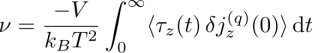
where ![]() is the heat current fluctuation.
is the heat current fluctuation.
Analogous formulas can be written for the other transport coefficients, either at equilibrium or out of equilibrium.
3.3.4. Analysis of the results
The simulations of Sarman have first introduced and validated a way to perform molecular simulations in constrained ensembles, opening the route to the simulation of transport coefficients in LCs (Sarman 1995). In particular, the use of Lagrange (or Gauss) multipliers to keep the director fixed, and the mechanical analog of the temperature gradient in a constant temperature simulations have been key steps.
The transport coefficients have been obtained from different ensembles, and using different methods, and they are consistent within the computation uncertainties. In particular, Sarman demonstrated numerically that the Leslie thermomechanical coefficient ν does exist in cholesterics. This is true even though the model is very simple, with molecules made up of rigid ellispoids.
The old simulation models were far from the experimental molecules, whereas the newer simulations are more and more realistic, with more realistic shapes and longer cholesteric pitches. Therefore, the new simulations allow us to go beyond the purely hypothetical systems and to put numbers in place of reduced units. Yet, there is still no quantitative agreement between these simulations and the experiments. The rigid Gay–Berne models tend to underestimate γ1 and overestimate ν. It should be possible in the future to use even more realistic, multigrain flexible molecules (Daivis and Evans 1994). This would allow for simulating molecules with a specific chemical structure, but this requires more computational power and more involved methods to impose the external constraints.
The latest simulations have shown that ν increases with the spontaneous twist q0 of the cholesteric, so that ![]() is constant for these simple systems. This is true whatever the shape of the ellipsoids (discotic or calamitic) and even for achiral nematics doped with chiral impurities.
is constant for these simple systems. This is true whatever the shape of the ellipsoids (discotic or calamitic) and even for achiral nematics doped with chiral impurities.
Finally, it is worth nothing that the simulations have never been performed on deformed nematics to compute the thermomechanical coefficients of Akopyan and Zel’dovich. However, it seems that at least twisted nematics could be simulated in the same way.
Sarman and co. also simulated uniform nematics under a temperature gradient and showed that the director experiences a torque (Sarman and Evans 1993; Sarman 1994; Sarman and Laaksonen 2014; Sarman et al. 2017, 2019). This torque is quadratic in ![]() of the form
of the form
and tends to align the director perpendicular to ![]() (in calamitic nematic and cholesteric LCs, μT < 0) or parallel to
(in calamitic nematic and cholesteric LCs, μT < 0) or parallel to ![]() (in discotic nematic LC, μT > 0). This orientation is the one which minimizes the irreversible energy dissipation rate. To our knowledge, the only experimental estimate of the thermo-orientational coefficient μT has been given in Demenev et al. (2009); Trashkeev and Britvin (2011): |μT| ∼ 3 × 10⁻¹¹ N/K2. However, our own estimate realized by attempting to reorient with a temperature gradient the director in a sample treated for sliding planar anchoring suggests that this value is largely overestimated and certainly less than 10−13 N/K2 (Oswald 2019). It is clear that more experiments are necessary to settle this issue.
(in discotic nematic LC, μT > 0). This orientation is the one which minimizes the irreversible energy dissipation rate. To our knowledge, the only experimental estimate of the thermo-orientational coefficient μT has been given in Demenev et al. (2009); Trashkeev and Britvin (2011): |μT| ∼ 3 × 10⁻¹¹ N/K2. However, our own estimate realized by attempting to reorient with a temperature gradient the director in a sample treated for sliding planar anchoring suggests that this value is largely overestimated and certainly less than 10−13 N/K2 (Oswald 2019). It is clear that more experiments are necessary to settle this issue.
3.4. Experimental evidence of the thermomechanical effect
This section is devoted to the experimental evidence of the TM effect in nematic and cholesteric LCs. The experiments can be categorized in two groups: the static experiments in which the director field is just distorted by the temperature gradient and the dynamic experiments in which the director constantly rotates under the action of the temperature gradient. The first experiments are delicate because the distortions caused by the non-equilibrium TM effects are extremely small and add to TM effects due to the temperature variations of the elastic constants. The Éber and Jánossy experiment belongs to this category. We will describe it in detail because it is the first experiment that revealed a non-equilibrium TM effect at the compensation temperature of a cholesteric phase. The dynamic experiments are more spectacular because they show more directly the non-equilibrium TM effect. Three experiments of this type will be described. The first two will concern the continuous rotation of the cholesteric helix in samples treated for sliding planar anchoring and mixed anchoring. The third experiment will deal with the drift of cholesteric fingers and the formation of spirals in homeotropic samples. It must be emphasized that in all the experiments described in this section, flows were never observed in the samples in spite of careful observations. For this reason, we will neglect them in the calculations, and will focus only on the resolution of the torque equation, directly responsible for the phenomena described here.
3.4.1. The static Éber and Jánossy experiment
3.4.1.1. A bit of history
As we already mentioned, it has long been believed that the Leslie TM effect was entirely responsible for the Lehmann effect (Lehmann 1900; Dequidt 2008; Oswald and Dequidt 2008b; Yamamoto et al. 2015; Ito et al. 2016). But this is wrong, as demonstrated by several experiments (Oswald 2012b; Poy 2017; Oswald and Poy 2018; Oswald et al. 2019b). For a review, see Oswald et al. (2019a). However, the first irrefutable experimental evidence of the Leslie TM effect in a cholesteric LC was reported by Éber and Jánossy (1982). This experiment was performed at the compensation temperature of a cholesteric phase, which raised a strong controversy with theorists, the latter claiming that the Leslie TM effect should disappear at this temperature (Pleiner and Brand 1987, 1988), while Éber and Jánossy found a non-zero effect at this temperature (Éber and Jánossy 1984, 1988). To make a decision about this issue, Padmini and Madhusudana (1993) conducted a new experiment to measure the electric analog νE of the thermomechanical coefficient ν in a compensated cholesteric mixture6. In doing this, they found that νE vanishes and changes sign at the compensation temperature, as proposed by theorists. As the same behavior should hold for the thermomechanical coefficient, they logically concluded that the Éber and Jánossy result was due to an artifact of measurement, thus putting a temporary end to the debate.
Temporary, because we redid these two experiments and found the same results as Éber and Jánossy on one side (Dequidt and Oswald 2007b; Dequidt et al. 2008) and Padmini and Madhusudana on the other side (Dequidt and Oswald 2007a), raising again a contradiction. To solve it, we analyzed in more detail the results of the Padmini and Madhusudana experiment and showed that they could not be explained in terms of electromechanical coupling, but resulted from a flexoelectric effect (Dequidt and Oswald 2007a). As for the Éber and Jánossy results, we realized that they were indeed compatible with the Leslie theory after noticing that the symmetry group of the cholesteric phase at the compensation temperature is D∞ (the phase remains chiral, not only at the microscopic scale, but also at the macroscopic scale), and not D∞h as in an usual nematic phase, in spite of the fact that the director field is unwound (Dequidt et al. 2008).

Figure 3.4. (a) Phase diagram of the mixture EM + CC. Along the dashed line, the cholesteric is compensated. It is left-handed (q0 < 0) on the left of this line and right-handed (q0 > 0) on the right. (b) Equilibrium twist as a function of temperature in the mixture EM + 45 wt% CC. Reproduced from Oswald (2012b) with kind permission of The European Physical Journal
3.4.1.2. Principle of the experiment and theoretical prediction
The original experiment by Éber and Jánossy was performed with a compensated cholesteric mixture. In such a mixture, there exists a temperature, called compensation temperature (Tc), at which the equilibrium twist vanishes and changes sign. Mixtures of usual nematics with the chiral dopant cholesteryl chloride (CC) often have this property. A typical example is shown in the phase diagram of Figure 3.4 where the nematic LC used is an eutectic mixture (EM) composed of 57 wt% of 8CB (4-n-octylcynaobiphenyl) and 43 wt% of 8OCB (4-n-octyloxycynaobiphenyl). Note that similar phase diagrams are observed with the mixtures 8CB + CC7 or 8OCB + CC, also used by Éber and Jánossy and ourselves. Experimentally, the compensated mixture is introduced between two parallel glass plates treated for strong homeotropic anchoring. This sample is then placed inside a temperature gradient parallel to the glass plates. In our own experiments, the directional growth apparatus described in Oswald et al. (1993) was used to impose the temperature gradient. In this geometry, the cholesteric helix unwinds when its pitch becomes larger than the sample thickness. As a result, a band of homeotropic “nematic phase”, centered on the compensation temperature, forms in the sample. This region is bordered by cholesteric fingers, which are very clear under the microscope as shown in Figure 3.5 (for a review about the helix unwinding in homeotropic samples, see Oswald et al. (2000) and Oswald and Pieranski (2005)).

Figure 3.5. Photo taken between crossed polarizers of a homeotropic sample subjected to a large temperature gradient. In the black band, the cholesteric phase is unwound because the pitch is larger than the thickness. This band is centered on the compensation temperature and is bordered by two regions filled with cholesteric fingers. The unwound zone is 465 μm wide. d = 40 μm and G = 51◦C/cm. Reproduced from Dequidt et al. (2008) with kind permission of The European Physical Journal
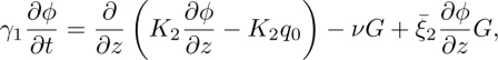
In practice, the director field in the homeotropic “nematic” band is a little distorted because of the presence of the temperature gradient. Two effects add here. The first one is due to the temperature variations of the elastic constants Ki and the equilibrium twist q0 of the cholesteric phase. This equilibrium effect is described by the contribution ![]() to the molecular field given in equation [3.14]. The second effect is due to the non-equilibrium Leslie, Akopyan and Zel’dovich thermomechanical forces
to the molecular field given in equation [3.14]. The second effect is due to the non-equilibrium Leslie, Akopyan and Zel’dovich thermomechanical forces ![]() given in equations [3.22] and [3.24], respectively. At equilibrium, the torque equation reads
given in equations [3.22] and [3.24], respectively. At equilibrium, the torque equation reads
where ![]() is the usual molecular field given by equation [3.13]. This equation is complicated, but can be simplified by noting that the director field is very little distorted. As a result, one can write that, to first order in distortion,
is the usual molecular field given by equation [3.13]. This equation is complicated, but can be simplified by noting that the director field is very little distorted. As a result, one can write that, to first order in distortion, ![]() by taking the x-axis along the temperature gradient and the z-axis perpendicular to the glass plates. In this limit, the previous equation becomes
by taking the x-axis along the temperature gradient and the z-axis perpendicular to the glass plates. In this limit, the previous equation becomes

which gives explicitly by noting that ![]()

with ![]()
In the previous equations, the second derivatives with respect to x can be neglected because the sample thickness d is always much smaller than the width of the nematic band (this can be checked a posteriori). Solving these equations by neglecting these derivatives gives (Dequidt 2008; Dequidt et al. 2008):
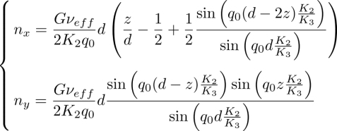
These formula generalize the solution given by Éber and Jánossy (1982) since they are still valid out of the compensation point Tc. In particular, they give back the spinodal limit for the nematic phase as nx and ny diverge when qd = π(K3/K2) or d/p = K3/(2K2) (Oswald et al. 2000; Oswald and Pieranski 2005).
The solution can be linearized in q0 in the vicinity of the compensation temperature Tc (at which q0 = 0), which gives:

This formula shows that measuring K3 and ny at Tc (where nx = 0) gives the effective coefficient ![]() . From this measurement and that of the corrective term
. From this measurement and that of the corrective term ![]() , the value at Tc of the thermomechanical Leslie coefficient ν can be obtained.
, the value at Tc of the thermomechanical Leslie coefficient ν can be obtained.
3.4.1.3. Experimental results
In practice, the distortion of the director field in the middle of the nematic band was obtained by measuring the phase shift ΦH between the extraordinary and ordinary components of a thin laser beam (5 μm in diameter at the waist), crossing the sample at this place. A straightforward calculation gives
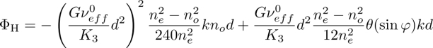
In this formula, no and ne are the ordinary and extraordinary refraction indices, k = 2π/λ is the angular wavenumber of the laser, θ is the angle (very small experimentally, but impossible to exactly cancel) between the beam and the normal to the sample and φ is the azimuthal angle of the beam with respect to the temperature gradient. This equation shows that at normal incidence (θ = 0), ΦH is proportional to G2 and d5, a result already given by Éber and Jánossy (1982). However, an additional term linear in G appears when the laser beam is slightly misaligned, but the term in G2 remains unchanged.
Experimentally, ΦH was measured by using a rotating analyzer, a quarter-wave plate, a photodiode and a lock-in amplifier following the method of Lim and Ho (1978). A typical curve measured with the compensated mixture 8OCB + 50wt% CC is shown in Figure 3.6. This curve, obtained with a sample of thickness d = 100 μm, is well fitted by a parabola of type aHG − bHG2, in agreement with equation [3.44]. Performing similar measurements with samples of different thicknesses showed that the fit parameter bH was proportional to d5 in agreement with equation [3.44]. From this measurement, a value of ![]() was obtained. Finally, K2 and
was obtained. Finally, K2 and ![]() were measured. From these data, it was found that in the mixture 8OCB + 50wt% CC, ν = (2.8 ± 0.6) × 10−7 kg K−1 s−2 at Tc. Note that in these experiments, great care was taken to determine the uncertainties by using the maximum-likelihood method each time a quantity was measured. This value of ν is close to the value obtained before by Éber and Jánossy in the mixture 8CB + 50 wt% CC. This confirmed that the Leslie thermomechanical coefficient does not vanish at the compensation temperature of a cholesteric phase.
were measured. From these data, it was found that in the mixture 8OCB + 50wt% CC, ν = (2.8 ± 0.6) × 10−7 kg K−1 s−2 at Tc. Note that in these experiments, great care was taken to determine the uncertainties by using the maximum-likelihood method each time a quantity was measured. This value of ν is close to the value obtained before by Éber and Jánossy in the mixture 8CB + 50 wt% CC. This confirmed that the Leslie thermomechanical coefficient does not vanish at the compensation temperature of a cholesteric phase.
3.4.2. Another static experiment proposed in the literature
The static Éber and Jánossy experiment was designed to measure the Leslie coefficient at the compensation temperature of a compensated mixture. In practice, other geometries could be considered to measure the thermomechanical coefficients, in particular the Akopyan and Zel’dovich coefficients in nematics. In this context, Akopyan and Zel’dovich, and later Poursamad, have proposed to impose a temperature gradient to a twisted nematic sample (Figure 3.7) and to measure the nz distortion of the director field (Akopyan and Zel’dovich 1984; Poursamad 2009). In that case, it can be shown by solving the torque equation in isotropic elasticity that, to the first order in nz:
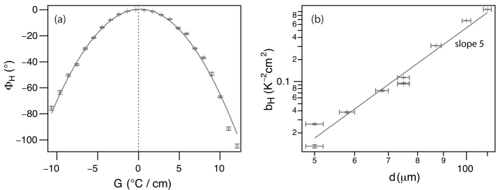
Figure 3.6. (a) Phase shift as a function of the temperature gradient when d = 100 μm. (b) Fit parameter bH as a function of the sample thickness showing that the d5-dependence is well satisfied. 8OCB + 50 wt% CC, homeotropic samples. Reproduced from Dequidt and Oswald (2007b)
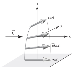
Figure 3.7. Geometry proposed by Poursamad to measure the Akopyan and Zel’dovich thermomechanical coefficients
As in the Éber and Jánossy experiment, two terms compete. The thermomechanical term, calculated by Akopyan and Zel’dovich and Poursamad, proportional to ![]() 4 and another term due to temperature variation of the Frank constant, neglected by these authors in their papers. At this level, it can be interesting to estimate these two terms. In order of magnitude
4 and another term due to temperature variation of the Frank constant, neglected by these authors in their papers. At this level, it can be interesting to estimate these two terms. In order of magnitude ![]() ∼ 1 pN/K, K ∼ 3 pN which gives by taking d = 100 μm and G = 3000 K/m
∼ 1 pN/K, K ∼ 3 pN which gives by taking d = 100 μm and G = 3000 K/m ![]() . This corresponds to a tilt angle of the director of about 2◦ with respect to the horizontal plane in the middle of the sample. For the thermomechanical term, all depends on the order of magnitude of the
. This corresponds to a tilt angle of the director of about 2◦ with respect to the horizontal plane in the middle of the sample. For the thermomechanical term, all depends on the order of magnitude of the ![]() ’s. According to Akopyan and Zel’dovich, these terms must be of the order of 10−11 N/K (Akopyan and Zel’dovich 1984). With this value, and the same as before for the other parameters, we calculate
’s. According to Akopyan and Zel’dovich, these terms must be of the order of 10−11 N/K (Akopyan and Zel’dovich 1984). With this value, and the same as before for the other parameters, we calculate ![]() which is considerable. It turns out that the
which is considerable. It turns out that the ![]() are much smaller experimentally, typically ranging between 10−15 and 10−14 N/K as we shall show later. This is why we think this experiment is not suitable for measuring the
are much smaller experimentally, typically ranging between 10−15 and 10−14 N/K as we shall show later. This is why we think this experiment is not suitable for measuring the ![]() in usual nematics. Finally, we mention that a similar calculation was conducted for a twisted nematic phase subjected to a two-dimensional temperature gradient (Poursamad and Hakobyan 2008).
in usual nematics. Finally, we mention that a similar calculation was conducted for a twisted nematic phase subjected to a two-dimensional temperature gradient (Poursamad and Hakobyan 2008).
3.4.3. Continuous rotation of translationally invariant configurations
While the Éber and Jánossy experiment is very elegant, it is very limited because it cannot be performed outside of the compensation temperature. In addition, this measurement is not direct since two TM effects are measured within the same time frame. Therefore, it was important to find alternative methods to eliminate these two problems. One of them was suggested by Leslie himself, who showed in his seminal paper (Leslie 1968) that the helix rotates at constant velocity in a temperature gradient when the director can freely rotate on the boundary of the cholesteric domain. This prediction was indeed confirmed by molecular dynamics simulations, as recalled in section 3.3.
In this section, we describe two experiments in which translationally invariant configurations (TIC) are set into continuous rotation by application of a temperature gradient. In practice, the cholesteric phase is sandwiched between two parallel glass plates and the temperature gradient is applied along the normal to the glass plates. In the first configuration, the two plates are treated for sliding planar anchoring, so that the helix is slightly deformed and orients parallel to the temperature gradient. This geometry will be referred to as Leslie geometry in the following. In the second configuration, one plate is treated for sliding planar anchoring, while the other is treated for homeotropic anchoring. In this case, the helix still orients parallel to the temperature gradient, but it is highly deformed. This will be referred to as mixed geometry in the following, where we show how to calculate the rotation velocity of a TIC in all generality.
3.4.3.1. TIC rotation velocity: a general formula
In practice, the LC sample of thickness d is sandwiched between two parallel glass plates of total thickness ![]() 8. The temperature gradient G is obtained by imposing a temperature difference ΔT between the two external top and bottom faces of the sample. As a result, the local gradient G in the LC is proportional to the imposed temperature gradient
8. The temperature gradient G is obtained by imposing a temperature difference ΔT between the two external top and bottom faces of the sample. As a result, the local gradient G in the LC is proportional to the imposed temperature gradient ![]() . We refer to Oswald and Dequidt (2008b) and Dequidt (2008) for a description of the setup used in experiments to impose the temperature gradient.
. We refer to Oswald and Dequidt (2008b) and Dequidt (2008) for a description of the setup used in experiments to impose the temperature gradient.
With the z-axis vertical and oriented upwards, the components of the director in a TIC are given by
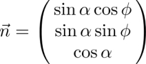
where the zenithal and azimuthal angles α and ϕ only depend on z since the system is supposed to be translationally invariant in the horizontal plane (x, y).
In the following, we show that the director rotates at constant angular velocity ω when a temperature gradient is applied along the z-axis, provided that the anchoring is sliding on the two glass plates. This rotation is due to the non-equilibrium TM torque that must equilibrate with the elastic and viscous torques in the stationary regime according to the general torque equation [3.8].
Two methods can be used to calculate this velocity. The first, used by Leslie (1968) and ourselves in Dequidt (2008); Dequidt et al. (2008); Oswald and Dequidt (2008a) and Oswald (2012b) consists of directly solving the torque equation [3.8] subjected to the boundary condition 3.12. This is quite easy to do with Leslie geometry when α = π/2. In this case, the bulk torque equation reduces to ![]() and reads explicitly
and reads explicitly
where the three contributions – elastic, viscous and thermomechanical – are easily recognizable. If the anchoring is sliding planar on the plates, this second-order differential equation must be solved with the boundary conditions
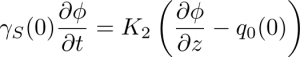
at the bottom plate z = 0 and

at the top plate z = d, with γS being the rotational surface viscosity.
Following Leslie (1968), we can look for a solution of the type ![]() . After substitution in the previous equations, we obtain
. After substitution in the previous equations, we obtain
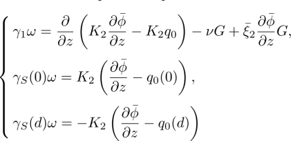
where G is the local temperature gradient given by ![]() by denoting by κg the thermal conductivity of the glass9. Integrating over the sample thickness, the first equation in [3.50] is written by using the two other equations and by assuming that the helix is slightly distorted
by denoting by κg the thermal conductivity of the glass9. Integrating over the sample thickness, the first equation in [3.50] is written by using the two other equations and by assuming that the helix is slightly distorted ![]() :
:
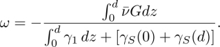
where ![]() is the effective Leslie coefficient, which is measured experimentally.
is the effective Leslie coefficient, which is measured experimentally.
If the sample is very thin, the material constants are almost constant inside the sample. In this limit, the previous equation becomes simply by setting ![]()
![]() :
:
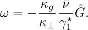
where the values of the material constants are taken at the average temperature of the sample.
The same calculation could be made in the general case, when ![]() but it is much more complicated. For this reason, we prefer another method, proposed in Dequidt et al. (2016), which does not need to explicitly solve the torque equation to find ω.
but it is much more complicated. For this reason, we prefer another method, proposed in Dequidt et al. (2016), which does not need to explicitly solve the torque equation to find ω.
The starting point of this calculation consists of noticing that the elastic energy of the cholesteric phase ![]() is constant during the rotation. Mathematically, this condition reads
is constant during the rotation. Mathematically, this condition reads
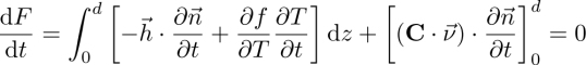
Replacing ![]() and C ·
and C · ![]() in this equation by their expressions given in equation [3.9] and [3.12], after noticing that
in this equation by their expressions given in equation [3.9] and [3.12], after noticing that ![]() in a TIC10 yields:
in a TIC10 yields:
Because ![]() , we obtain from this equation by using equation [3.46] and the expressions [3.22] and [3.24] of the Leslie and Akopyan and Zel’dovich forces
, we obtain from this equation by using equation [3.46] and the expressions [3.22] and [3.24] of the Leslie and Akopyan and Zel’dovich forces

where

In these formulas, the temperature gradient G depends on z in general. It is obtained by writing that the heat flux is the same in the sample and in the glass plates. Using equation [3.32], this gives:
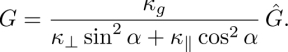
Equations [3.55]–[3.57] generalize to any TIC the formula [3.51], obtained in the Leslie geometry. They show that, in the general case, the rotation velocity of the helix only depends on the three non-equilibrium TM coefficients ν, ![]() . A very important point is that the rotation disappears when these coefficients vanish. This shows that the static equilibrium TM contribution
. A very important point is that the rotation disappears when these coefficients vanish. This shows that the static equilibrium TM contribution ![]() to the molecular field cannot be responsible for the rotation of the helix in a TIC and contributes just to its deformation during the rotation. This is a major advantage with respect to the Éber and Jánossy experiment in which both effects – equilibrium STM and non-equilibrium TM – played the same role and should be separated.
to the molecular field cannot be responsible for the rotation of the helix in a TIC and contributes just to its deformation during the rotation. This is a major advantage with respect to the Éber and Jánossy experiment in which both effects – equilibrium STM and non-equilibrium TM – played the same role and should be separated.
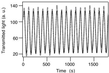
Figure 3.8. Transmitted intensity between crossed polarizers. Crosses are experimental points and the curved solid line is the best fit to a sinusoidal law of period 100 s. Reproduced from Dequidt et al. (2008) with kind permission of The European Physical Journal
3.4.3.2. Experimental results with the compensated mixtures in the Leslie geometry
The goal of these experiments was to directly evidence the TM effect predicted by Leslie in 1968. To perform them, a specific surface treatment of the glass plates, allowing a sliding planar anchoring of the LC molecules, was developed in collaboration with Żywoćinski (Oswald et al. 2008). This surface treatment – which consists of the deposition by spin coating of a thin layer of a viscoelastic polymer11 – was fully characterized. In particular, its surface viscosity was measured (Oswald 2012a; Oswald and Poy 2013) and the problems of memorization that occur when the director stops rotating, or rotates very slowly, were described in Oswald (2014a).
In sliding planar samples, a great number of defects can form since the anchoring direction is degenerated. In practice, most of the defects are ![]() disclination lines, even if ±1 defects are sometimes observed. These defects usually nucleate in large number when the sample is cooled down from the isotropic liquid. As the anchoring is sliding, most of the defects annihilate (Oswald et al. 2008) but some of them can remain in the sample after annealing because they are pinned on a dust particle or a surface defect. In the following, we begin with a description of what happens in the samples far from the defects, in regions where the in-plane distortions of the director field are negligible. We will then study the director rotation in the vicinity of disclination lines and in the presence of a surface defect. Finally, we will show that it is possible to stop the rotation of the director by applying an electric field and we will describe the final state of the sample once the director has stopped rotating.
disclination lines, even if ±1 defects are sometimes observed. These defects usually nucleate in large number when the sample is cooled down from the isotropic liquid. As the anchoring is sliding, most of the defects annihilate (Oswald et al. 2008) but some of them can remain in the sample after annealing because they are pinned on a dust particle or a surface defect. In the following, we begin with a description of what happens in the samples far from the defects, in regions where the in-plane distortions of the director field are negligible. We will then study the director rotation in the vicinity of disclination lines and in the presence of a surface defect. Finally, we will show that it is possible to stop the rotation of the director by applying an electric field and we will describe the final state of the sample once the director has stopped rotating.
3.4.3.2.1. Rotation in a homogeneous sample
The first experiment in the Leslie geometry was performed with a compensated mixture of 8OCB + 50 wt%CC (Dequidt et al. 2008). This choice was driven by the Éber and Jánossy experiment that showed the existence of a TM Leslie effect at the compensation temperature of this mixture. In order to measure the rotation velocity of the director, a 10-μm-thick sample was prepared. This sample was then placed in the setup, described in Oswald and Dequidt (2008b), to impose a temperature gradient and was observed in the polarizing microscope. By doing so, it was found that, at the compensation temperature, the transmitted intensity between crossed polarizers was oscillating in time in a sinusoidal manner (Figure 3.8), revealing that the director was rotating at constant velocity in the sample. For the first time, this showed the existence of the TM Leslie effect at the compensation temperature, in a direct way.
The experiment was then performed at other temperatures from both sides of the compensation temperature (Oswald and Dequidt 2008a). An important point was the sense of rotation of the helix. It was determined by looking at the direction in which the polarizers should be rotated to maintain a constant intensity (another method will be described later). The result of these measurements is shown in Figure 3.9. As we can see, the sense of rotation is the same on both sides of the compensation temperature, counterclockwise (ω > 0) when the temperature gradient is directed downwards (ΔT < 0) and clockwise when the temperature gradient is directed upwards (ΔT > 0). The experiment also showed that ω is proportional to ΔT in agreement with formula [3.51]. From these measurements, the coefficient ![]() was deduced after the ratio κg/κ⊥ and the viscosity
was deduced after the ratio κg/κ⊥ and the viscosity ![]() were measured. At Tc, it was found that κg/κ⊥ ≈ 7, γ1 ≈ 0.075 Pa s and γS ≈ 3.2 × 10⁻⁷ Pa s m, which led to
were measured. At Tc, it was found that κg/κ⊥ ≈ 7, γ1 ≈ 0.075 Pa s and γS ≈ 3.2 × 10⁻⁷ Pa s m, which led to ![]() = ν ≈ 1 × 10⁻⁷ kg K−1 s−2. This value is compatible with that previously found in the Éber and Jánossy experiment. The curve shown in Figure 3.9(a) also suggests that
= ν ≈ 1 × 10⁻⁷ kg K−1 s−2. This value is compatible with that previously found in the Éber and Jánossy experiment. The curve shown in Figure 3.9(a) also suggests that ![]() changes little with temperature. Indeed, the viscosity decreases when the temperature increases, which could explain, in large part, why the velocity increases when the temperature increases. This was checked in minute detail in the mixture EM + 50 wt% CC in which the two viscosities γ1 and γS were measured as a function of temperature. In this mixture it was found that, within experimental errors,
changes little with temperature. Indeed, the viscosity decreases when the temperature increases, which could explain, in large part, why the velocity increases when the temperature increases. This was checked in minute detail in the mixture EM + 50 wt% CC in which the two viscosities γ1 and γS were measured as a function of temperature. In this mixture it was found that, within experimental errors, ![]() was approximately constant, of the order of 1×10⁻⁷ kg K−1 s−2 in a temperature interval of 10◦C below the clearing temperature. This value is comparable with that found at the compensation temperature in the 8OCB + 50 wt% CC mixture (Oswald 2012b), studied previously. The independence of
was approximately constant, of the order of 1×10⁻⁷ kg K−1 s−2 in a temperature interval of 10◦C below the clearing temperature. This value is comparable with that found at the compensation temperature in the 8OCB + 50 wt% CC mixture (Oswald 2012b), studied previously. The independence of ![]() with the temperature also suggests that the macroscopic Akopyan and Zel’dovich contribution to
with the temperature also suggests that the macroscopic Akopyan and Zel’dovich contribution to ![]() is negligible in these mixtures in which q0 changes a lot with temperature. This point will be confirmed later.
is negligible in these mixtures in which q0 changes a lot with temperature. This point will be confirmed later.

Figure 3.9. (a) Angular velocity as a function of the sample temperature measured when ΔT = −40◦C. (b) Angular rotation velocity as a function of the temperature difference measured at T = Tc. Mixture 8OCB + 50 wt% CC, d = 25 μm. Reproduced from Oswald and Dequidt (2008a)
More recently, we made similar measurements in diluted cholesteric mixtures12 (Oswald 2014b). In these mixtures, the pitch was chosen to be of the same order of magnitude as in the previously studied zcompensated mixtures at the clearing temperature. Although the pitch was similar (between 5 and 10 μm, in practice), we found that ![]() was much smaller (typically, 50 times smaller) in these mixtures than in the compensated mixtures. An example of systematic measurements with a diluted mixture of 7CB (4-n-heptylcyanopbiphenyl) and R811 (R-(+)-octan-2-yl 4-((4-(hexyloxy)benzoyl)oxy)benzoate) is shown in Figure 3.10. These data show that
was much smaller (typically, 50 times smaller) in these mixtures than in the compensated mixtures. An example of systematic measurements with a diluted mixture of 7CB (4-n-heptylcyanopbiphenyl) and R811 (R-(+)-octan-2-yl 4-((4-(hexyloxy)benzoyl)oxy)benzoate) is shown in Figure 3.10. These data show that ![]() is proportional to the concentration C of chiral molecules at low concentration. This result was expected since
is proportional to the concentration C of chiral molecules at low concentration. This result was expected since ![]() must vanish when C → 0 and led us to define the Leslie thermomechanical power
must vanish when C → 0 and led us to define the Leslie thermomechanical power
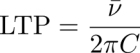
by analogy with the helical twist power defined to be
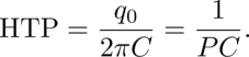
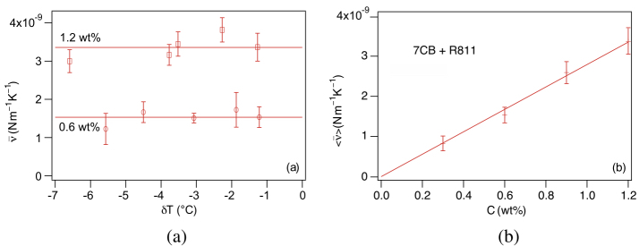
Figure 3.10. (a) Effective Leslie coefficient  as a function of temperature (δT = T − TChI) measured in the diluted mixtures 7CB + 0.6wt% R811 and 7CB + 1.2wt% R811. (b) Average value of as a function of the concentration of chiral molecules. Reproduced from Oswald (2014b)
Typical values of the HTP and the LTP are given in Table 3.1 for the mixtures 7CB + R811, 7CB + CC, MBBA + R811 and MBBA + CC, where MBBA is the N-(p-methoxy-benzylidene)-p-butylaniline, the first known LC with a nematic phase at room temperature. This table shows that the LTP crucially depends on the chiral molecule chosen, but also on the host nematic LC. For instance, the LTP of the R811 is always positive and three times larger in 7CB than in MBBA. In comparison, the LTP of the CC is smaller in absolute value, although still larger in 7CB than in MBBA. On the other hand, the LTP of the CC is positive in 7CB and negative in MBBA. These results show that there is no direct relationship between the HTP and the LTP, i.e. between the spontaneous twist q0 and the effective Leslie thermomechanical coefficient ![]() This appears more clearly still if we calculate the ratio R=LTP/HTP=
This appears more clearly still if we calculate the ratio R=LTP/HTP= ![]() which is very different from one mixture to another (Table 3.1). This is not surprising as the HTP is a static property of the phase, whereas the LTP is dynamic in nature.
which is very different from one mixture to another (Table 3.1). This is not surprising as the HTP is a static property of the phase, whereas the LTP is dynamic in nature.
Table 3.1. Average values of the LTP (in unit of 10−8 N m−1 K−1wt%−1) of the HTP (in μm−1wt%−1) and of the R-ratio (in fN K−1)
|
LC |
7CB |
7CB |
MBBA |
MBBA |
|
Dopant |
R811 |
CC |
R811 |
CC |
|
LTP=¯ν/(2πC) |
4.3 |
1.2 |
1.5 |
-0.4 |
|
HTP=q0/(2πC) |
12.1 |
-2.9 |
10.2 |
-6,1 |
|
R=¯ν/q0 |
3.6 |
-4.2 |
1.5 |
0.6 |
The next step is to determine whether it is the microscopic term of Leslie ν or the macroscopic term of Akopyan and Zel’dovich ![]() that is the more important in
that is the more important in ![]() . The only way to answer this question is to measure the order of magnitude of the Akopyan and Zel’dovich TM coefficients
. The only way to answer this question is to measure the order of magnitude of the Akopyan and Zel’dovich TM coefficients ![]() . This problem will be discussed at the end of this section. But before this, we analyze the behavior of the defects in the Leslie geometry.
. This problem will be discussed at the end of this section. But before this, we analyze the behavior of the defects in the Leslie geometry.
3.4.3.2.2. Rotation in the presence of disclination lines
In the previous section, we mentioned that disclination lines are often present in samples. In practice, they are almost impossible to completely eliminate. Hence the question as to whether their presence could disturb the velocity measurements.
To answer this question, we observed the rotation of the extinction branches of ±1/2 disclination lines that usually form in the samples and we simultaneously recorded the intensity transmitted between crossed polarizers at different places of the sample. In doing so, we observed that the director was rotating everywhere at the same velocity, as if the sample was homogeneous. An example of such measurements is shown in Figure 3.11. This photo was taken in a sample of the mixture EM+45 wt%CC at a temperature close to the compensation temperature under a temperature gradient ΔT = 40◦C. In this case, the director was rotating clockwise so that the extinction branches of the -1/2 lines rotated clockwise while those of the +1/2 lines rotated counterclockwise13.
We now calculate the rotation velocity of the director in the presence of disclination lines. In this case, angle ϕ between the director and the x-axis not only depends on z, but also on x and y, which makes the problem very complicated. To simplify the calculations, we assume first that the material constants do not depend on z and that K = K1 = K2 = K3 = −K4 (isotropic elasticity). With these hypotheses, the elastic energy reads simply
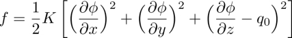

Figure 3.11. Typical texture observed between crossed polarizers with the mixture EM+45 wt% CC at a temperature close to the compensation temperature when the two glass plates are treated for sliding planar anchoring. The three graphs show the average intensity measured as a function of time inside the three squares marked 1, 2 and 3 on the photo. ΔT = 40◦C and d = 20 μm. The black bar is 100 μm long
and the bulk and surface torque equations [3.47]–[3.49] become

Integrating the first equation over the sample thickness yields an equation for the average angle ![]() by using the two boundary conditions:
by using the two boundary conditions:

where ![]() and
and ![]() . coordinates (r, θ), this equation reads
. coordinates (r, θ), this equation reads

An obvious solution is ![]() . For integer or half-integer m, this solution has no singularity in the plane θ = 0 and represents a disclination of topological rank m.
. For integer or half-integer m, this solution has no singularity in the plane θ = 0 and represents a disclination of topological rank m.
This calculation shows that, in isotropic elasticity, the presence of a disclination line does not change the rotation velocity of the molecules, whatever the rank of the line.
This is indeed observed experimentally with the ±1/2 lines. However, the situation is different for ±1 lines, as shown in the sequence of photos in Figure 3.12(a). If the extinction branches of the -1 line still rotate regularly, the branches of the +1 line rotate in a very irregular way while distorting heavily close to the core of the line. This effect is also visible in Figures 3.12(b) and (c), where we can see that the intensity measured close to the +1 line varies in an irregular way, contrary to that measured close to the -1 line.
It turns out that this effect is due to the elastic anisotropy of the LC neglected so far in the calculations. This can be seen immediately by looking at how the energy of a disclination line of rank m varies during the rotation. To perform this calculation, we need the expression of the elastic energy per unit surface area of the sample. At the compensation temperature, the director field is very slightly twisted along z and we can neglect the twist energy with respect to the splay and bend energies of expressions
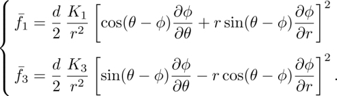
where ϕ is assumed not to depend on z. From these formulas, the energy Em = ![]() of a disclination line of rank m, core radius rc and external radius R can be calculated. By taking ϕ = mθ + ωt, we obtain:
of a disclination line of rank m, core radius rc and external radius R can be calculated. By taking ϕ = mθ + ωt, we obtain:
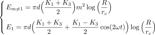

Figure 3.12. (a) Nine photographs taken at the compensation temperature showing the rotation of the four extinction branches of a pair of disclination lines of strength m = ±1. The two lines are 52 μm apart. Crossed polarizers, d ≈ 7.1 μm and G ≈ −70 000 K/m. (b and c) Intensity as a function of time recorded inside the white and black squares, respectively. On the top curve, the time at which each photo, numbered 1 to 9, was taken is indicated. EM + 45%CC. Reproduced from (Oswald 2012b) with kind permission of The European Physical Journal
This very simple calculation shows that for all disclination lines of rank m≠1 the energy does not change in time when the director rotates. By contrast, a +1 line oscillates between a radial configuration of energy πdK1 ln(R/rc) and a circular configuration of different energy πdK3 ln(R/rc) if K1 ![]() K3. This change of energy is responsible for the irregular rotation of the extinction branches of the +1 defect.
K3. This change of energy is responsible for the irregular rotation of the extinction branches of the +1 defect.
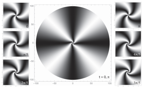
Figure 3.13. Numerical simulation of the deformation of the extinction branches of a +1 line during rotation by an angle π of the director. The central picture shows that the extinction branches are mainly deformed close to the core of the line. The six smaller pictures show their aspect over time inside the dashed square (of side length 10 in units of L) drawn in the central picture. Time is indicated on each of picture in units of τ
This result can be shown in a more compelling way by numerically solving the torque equation around a +1 line. By setting ϕ = θ + φ(r, t), the torque equation is written in the form
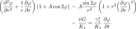
where ![]() is the elastic anisotropy factor. By choosing as the length scale
is the elastic anisotropy factor. By choosing as the length scale ![]() and as the time scale
and as the time scale ![]() 14, the previous equation is written in the dimensionless form
14, the previous equation is written in the dimensionless form

where r′ ≡ r/L and t′ ≡ t/τ. This equation in ϕ(r′,t′) was solved numerically with Mathematica by taking as boundary conditions ϕ(r′, 0) = 0 and ∂r′ ϕ(r′,t′) = 0 at ![]() and r′ = 100 (these two boundary conditions reflect the fact that the director is free to rotate on the core of radius
and r′ = 100 (these two boundary conditions reflect the fact that the director is free to rotate on the core of radius ![]() and far from the core at r′ = 100). The core radius can be estimated by assuming that the director escapes along the z-axis inside the core, in order to suppress the singularity. In doing so, the molecules are homeotropically anchored on the plates in the core, which costs anchoring energy. Minimizing the core energy with these assumptions yields
and far from the core at r′ = 100). The core radius can be estimated by assuming that the director escapes along the z-axis inside the core, in order to suppress the singularity. In doing so, the molecules are homeotropically anchored on the plates in the core, which costs anchoring energy. Minimizing the core energy with these assumptions yields ![]() where lp = K1/Wa is the extrapolation anchoring length of the sliding planar anchoring. Typical values for the compensated mixture used here are K1 = 3 pN, K3/K1 = 1.7 (A = 0.41) and Wa = 3 × 10⁻⁵ J/m2 (Oswald et al. 2008) and
where lp = K1/Wa is the extrapolation anchoring length of the sliding planar anchoring. Typical values for the compensated mixture used here are K1 = 3 pN, K3/K1 = 1.7 (A = 0.41) and Wa = 3 × 10⁻⁵ J/m2 (Oswald et al. 2008) and ![]() = 10−7 kg K−1 s−2, which gives, by taking G = 7 × 10⁴ K/m (ΔT = 40◦C) and d = 7.5 μm, L ≈ 20 μm, τ
= 10−7 kg K−1 s−2, which gives, by taking G = 7 × 10⁴ K/m (ΔT = 40◦C) and d = 7.5 μm, L ≈ 20 μm, τ ![]() 10 s and
10 s and ![]() 0.02 (in dimensionless unit). From this numerical solution, the aspect between crossed polarizers of the line can be calculated at different times, as shown in Figure 3.13. This simulation reproduces the observations fairly well. It shows that the extinction branches are deformed and rotate jerkily inside a disk of typical radius 5L.
0.02 (in dimensionless unit). From this numerical solution, the aspect between crossed polarizers of the line can be calculated at different times, as shown in Figure 3.13. This simulation reproduces the observations fairly well. It shows that the extinction branches are deformed and rotate jerkily inside a disk of typical radius 5L.
3.4.3.2.3. Rotation in the presence of an anchoring defect
In practice, it may happen that the polymercaptan layer dewets locally on the glass plates. This leads to a localized surface defect around which the extinction fringes of the director field form rings. One example is shown in Figure 3.14(a) where one can also see a -1/2 disclination line between crossed polarizers. This sequence of 10 photos, taken at a time interval of 10 s, shows that under the action of the temperature gradient, the rings continuously move inwards and collapse in the center of the defect, while the two extinction branches of the neighboring disclination line rotate at constant velocity.
In addition, a time recording of the local intensity measured in the vicinity of the defects shows that the director rotates at constant velocity, as if the sample was homogeneous. This observation indicates that the surface defect, just like the -1/2 disclination line, does not change the rotation velocity of the director.
To demonstrate this result, we solved the torque equation [3.63] for the average angle ![]() with a surface defect placed at the origin. To model this defect, we assumed that the viscosity
with a surface defect placed at the origin. To model this defect, we assumed that the viscosity ![]() is a function of r of the type:
is a function of r of the type:
where r0 represents the typical radius of the defect. Solving this problem with Mathematica yields
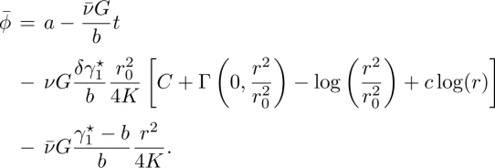
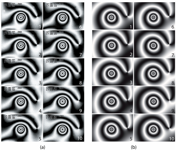
Figure 3.14. (a) Typical texture observed between crossed polarizers in the presence of a surface defect and a -1/2 disclination line. Each photo is 450 μm wide. (b) Texture calculated numerically from the complete solution. Reproduced from Dequidt et al. (2008) with kind permission of The European Physical Journal
In this expression, C is the Euler constant, Γ the incomplete Euler function, and a, b and c are integration constants. In order that φ does not diverge at the center of the defect, we must take c = 0. Constant a corresponds to a phase shift. It may be removed by changing the time origin. In the following, we shall take a = 0. Finally, we must take b = γ1 to cancel the torque ∂ϕ/∂r at infinity. With this choice of the constants, the solution reads
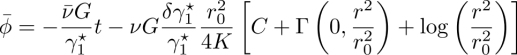
This formula shows:
1) that the director rotates everywhere with velocity ![]() whatever the “strength”
whatever the “strength” ![]() of the defect, as if the sample was homogeneous;
of the defect, as if the sample was homogeneous;
2) that the director winds radially inwards around the defect, which explains the fringes observed between crossed polarizers around the defect, the number of which is proportional to ![]() .
.
To this solution, one can add the solution to the torque equation −θd/2 corresponding to the -1/2 disclination line visible in Figure 3.14(a), where θd is the polar angle measured from the core of this line. The texture between crossed polarizers calculated from the complete solution is shown in Figure 3.14(b). In this calculation, the “strength” ![]() of the defect was chosen in order that the number of rings was approximately the same as in the experiment.
of the defect was chosen in order that the number of rings was approximately the same as in the experiment.
3.4.3.2.4. Rotation in the presence of an electric field
In this section, we describe an alternative method to measure the effective Leslie coefficient ![]() with an electric field. This measurement was performed in the Leslie geometry with the compensated mixture EM + 45 wt% CC. This LC is of positive dielectric anisotropy. The AC electric field (f = 10 kHz) was imposed by applying a voltage difference ΔV between two ITO electrodes deposited on the bottom plate at 2 mm apart (Figure 3.15(a)). As a result, the electric field is parallel to the glass plates and perpendicular to the edges of the insulating band separating the two electrodes. A calculation shows that the field is constant to better than 5%, given by
with an electric field. This measurement was performed in the Leslie geometry with the compensated mixture EM + 45 wt% CC. This LC is of positive dielectric anisotropy. The AC electric field (f = 10 kHz) was imposed by applying a voltage difference ΔV between two ITO electrodes deposited on the bottom plate at 2 mm apart (Figure 3.15(a)). As a result, the electric field is parallel to the glass plates and perpendicular to the edges of the insulating band separating the two electrodes. A calculation shows that the field is constant to better than 5%, given by ![]() , in the central part of width ∼ W/4 of the insulating band. For this reason, all measurements were performed in this region of the sample. Because the LC used is of positive dielectric anisotropy, its director tends to spontaneously align along the electric field. As a result, the electric field can be used to stop the rotation of the helix when a temperature gradient G is applied. From the measurement of the minimal electric field Estop, required to stop the rotation, the value of
, in the central part of width ∼ W/4 of the insulating band. For this reason, all measurements were performed in this region of the sample. Because the LC used is of positive dielectric anisotropy, its director tends to spontaneously align along the electric field. As a result, the electric field can be used to stop the rotation of the helix when a temperature gradient G is applied. From the measurement of the minimal electric field Estop, required to stop the rotation, the value of ![]() was deduced.
was deduced.
In practice, Estop was measured by recording the intensity between crossed polarizers as a function of time. Without an electric field, the intensity varies in a sinusoidal manner as shown in Figure 3.15(b). When the field is applied, the rotation becomes irregular, slowing down when the director is parallel to the field and accelerating when the director is perpendicular to the field (Figures 3.15(c) and (d)). As a result, the period of rotation Θ increases to finally diverge at Estop. In practice, Estop was measured by extrapolating to zero the curve of average angular velocity ![]() . Knowing Estop, the value of
. Knowing Estop, the value of ![]() was then calculated by numerically
was then calculated by numerically
solving the torque equation in the static regime.
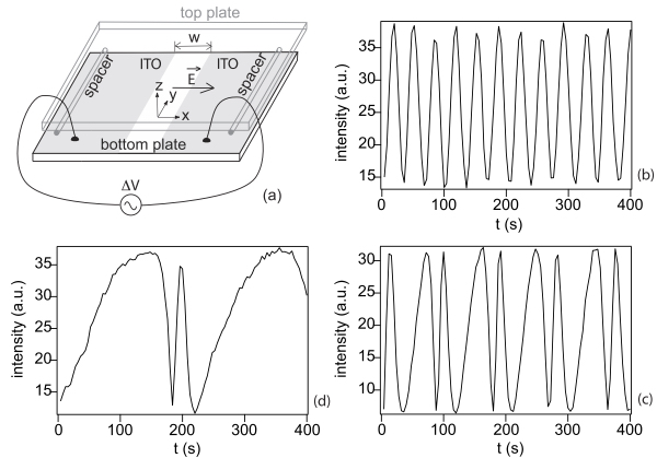
Figure 3.15. (a) Schematic of the cell used to impose an electric field. (b–d) Transmitted intensity between crossed polarizers as a function of time when E = 0, 12 900, 17 000 V/m. EM + 45%CC. d = 7 μm, T = Tc. Reproduced from Oswald (2012b) with kind permission of The European Physical Journal
The procedure was as follows. In the static regime (when E > Estop), the torque equation reads:

This equation is subjected to boundary conditions ![]() = q0(d) at z = d. In this equation, q0 and K2 are functions of z because they depend on temperature. In the compensated mixture, K2 is, within experimental errors, a linear function of T so that one can write
= q0(d) at z = d. In this equation, q0 and K2 are functions of z because they depend on temperature. In the compensated mixture, K2 is, within experimental errors, a linear function of T so that one can write ![]() After substitution in the previous equation and assuming
After substitution in the previous equation and assuming ![]() , we obtain
, we obtain
The general solution of this equation has the form:
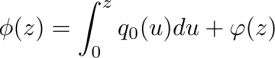
After substituting into equation [3.72], we obtain an equation for φ:

with ![]() = 0 at z = 0 and z = d. In this equation, K2, εa and the integral of q0 are known functions of z as their temperature variations are known. The value of
= 0 at z = 0 and z = d. In this equation, K2, εa and the integral of q0 are known functions of z as their temperature variations are known. The value of ![]() is obtained by setting E = Estop in this equation and by searching numerically for the largest value of
is obtained by setting E = Estop in this equation and by searching numerically for the largest value of ![]() for which this equation has a solution. This method confirmed that
for which this equation has a solution. This method confirmed that ![]() was constant between Tc and the melting temperature, of the order of 1.2 × 10⁻⁷ N/m/K, in good agreement with dynamical measurements.
was constant between Tc and the melting temperature, of the order of 1.2 × 10⁻⁷ N/m/K, in good agreement with dynamical measurements.
We end this paragraph by noting that π-walls can form and propagate in the sample when the electric field is larger than Estop. Each wall separates two zones in which the director is uniformly oriented and does not rotate. On the other hand, the wall propagation allows the director to rotate everywhere, even above Estop. From this point of view, these walls (or solitons) behave like dislocations in plasticity. Such walls are shown in Figure 3.16 when the temperature is equal to the compensation temperature. In this particular case, the director makes a constant angle with the electric field in each domain and rotates by ±π across each wall. The experiment showed that these walls propagate with a constant velocity that decreases when the electric field increases.
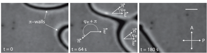
Figure 3.16. π-walls propagating when E/Estop ≈ 1.6. The intensity of the background is constant, which indicates that the director does not rotate out of the walls. T = Tc, d = 10 μm, Estop ≈ 2 × 10⁴ V/m and G = 7 × 10⁴ K/m. The white bar is 50 μmlong. Reproduced from Oswald (2012b) with kind permission of The European Physical Journal
To understand this behavior and predict the velocity of a soliton, we must solve the torque equation close to Tc for the average angle ![]() by taking into account the electric field. Because
by taking into account the electric field. Because ![]() close to Tc, this equation reads by assuming isotropic elasticity:
close to Tc, this equation reads by assuming isotropic elasticity:
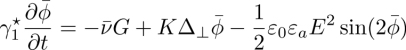
When G = 0, this equation has a solution of type

where ![]() is the electric coherence length. This equation describes a stationary π-wall of width
is the electric coherence length. This equation describes a stationary π-wall of width ![]() perpendicular to the x-axis. Note that here the x-axis can make an arbitrary
perpendicular to the x-axis. Note that here the x-axis can make an arbitrary ![]() angle with the electric field from which the angle is referred. For this static solution,
angle with the electric field from which the angle is referred. For this static solution, ![]()
A similar solution still exists when ![]() but now the wall propagates (Dauxois and Peyrard 2006). In this case, the solution must be searched in the form
but now the wall propagates (Dauxois and Peyrard 2006). In this case, the solution must be searched in the form ![]() where V is the wall velocity along the x-axis. In the frame of the wall (X = x − Vt), the torque equation rewrites in the from
where V is the wall velocity along the x-axis. In the frame of the wall (X = x − Vt), the torque equation rewrites in the from

Multiplying this equation by ![]() and integrating between −∞ and +∞ gives, by noting that
and integrating between −∞ and +∞ gives, by noting that ![]() and
and ![]() :
:
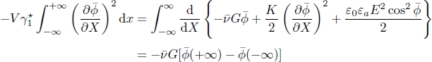
This gives the general formula
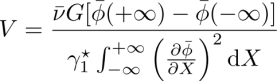
For a soliton-like solution such that ![]()
![]() , where
, where ![]() is the static solution obtained by equilibrating the thermomechanical torque with the electric torque:
is the static solution obtained by equilibrating the thermomechanical torque with the electric torque: ![]() , this formula gives:
, this formula gives:

At a small temperature gradient, the solution of equation [3.77] can be found in the form ![]() where
where ![]() is a small parameter (of the order of 0.2 in experiments) and
is a small parameter (of the order of 0.2 in experiments) and ![]() is given in equation [3.76]. By using equations [3.80] and [3.76] and by limiting the calculation to first order in this gives:
is given in equation [3.76]. By using equations [3.80] and [3.76] and by limiting the calculation to first order in this gives:

Note that the sign of the velocity depends on the sense of rotation of the director across the wall. This formula predicts that the wall velocity decreases when the electric field increases, in agreement with observations. We can also compare the velocity of the wall measured experimentally, in the order of 0.8 μm/s when E = 3.2104 V/m and G = 70 000 K/m, with the value of 0.94 μm/s calculated from the previous formula by taking ![]() Pa s and ν = 1.2 × 10⁻⁷ N/m/K. These two values are close, which confirms the value of
Pa s and ν = 1.2 × 10⁻⁷ N/m/K. These two values are close, which confirms the value of ![]() given above.
given above.
3.4.3.3. Experimental results with the diluted mixtures in the Leslie and mixed geometries
The experiments in the Leslie geometry just allow the measurement of the effective Leslie coefficient ![]() . In the compensated mixtures, we suspect that the AZ term
. In the compensated mixtures, we suspect that the AZ term ![]() coming from the macroscopic twist of the director field is negligible against the microscopic Leslie term ν coming from the chirality of the phase and the molecules. The situation is certainly different in diluted mixtures in which these two contributions could be of the same order of magnitude because of the small concentration of chiral molecules.
coming from the macroscopic twist of the director field is negligible against the microscopic Leslie term ν coming from the chirality of the phase and the molecules. The situation is certainly different in diluted mixtures in which these two contributions could be of the same order of magnitude because of the small concentration of chiral molecules.
To check this point, we measured the rotation velocity of a TIC in the Leslie and mixed geometries. According to our previous calculations, the rotation velocities must be different in these two geometries at equal external temperature gradient Ĝ. This is for two reasons: the first being that the local temperature gradient is different in the two configurations because of the anisotropy of the thermal conductivity15; and the second being that ω depends on ν and ![]() in the Leslie geometry and on ν,
in the Leslie geometry and on ν, ![]() and
and ![]() in the mixed geometry. Indeed, we recall that the rotation velocity in the Leslie geometry is given by
in the mixed geometry. Indeed, we recall that the rotation velocity in the Leslie geometry is given by

where ![]() and by
and by
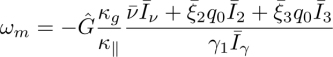
in the mixed geometry where we defined the new dimensionless integrals
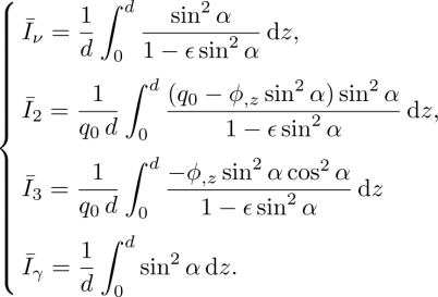
where α and ϕ are defined in equation [3.46] and ϵ = 1 − κ⊥/κ‖ is the relative anisotropy of thermal conductivity. These expressions were obtained from equation [3.51] and equations [3.55]–[3.56] by assuming that the material constants do not depend on z and by neglecting the surface viscosity γS. By eliminating ![]() between equations [3.82] and [3.83], we obtain
between equations [3.82] and [3.83], we obtain
This quantity gives the order of magnitude of the Akopyan and Zel’dovich coefficients ξi if we assume that they are all equal: ξ = ξ2 = ξ3 = ξ4. In that case, ![]() which gives
which gives ![]() .
.
Table 3.2. Values at the transition temperature of the main physical constants of the liquid crystal CCN-37
|
Constants |
K1 (pN) |
K2(pN |
K3 (pN |
κg κ |
κg κ⊥ |
γ1 (Pa s) |
|
Values at TChI |
0.96 |
0.84 |
1.37 |
5.1 |
7.4 |
0.0079 |
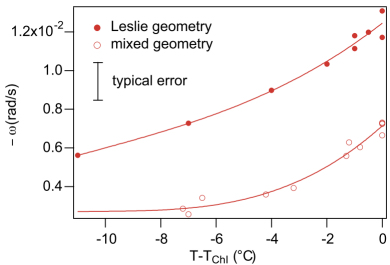
Figure 3.17. Angular velocity as a function of temperature measured in the Leslie and mixed geometries, with the mixture CCN-37 + 3 wt% CC. ΔT = 40◦C and d = 10.7 μm. Reprinted from Oswald et al. (2017) with the kind permission of Taylor & Francis
To perform this experiment, the LC CCN37 (4α,4’α-propylheptyl-1α, 1’α-bicyclo-hexyl-4β-carbonitrile) was chosen because it dissolves much less of the polymercaptan used for the sliding anchoring than MBBA, or the cyanobiphenyls used before. Because of this property, the anchoring continues to slide much longer (up to 3 days, instead of just a few hours), which greatly facilitates the velocity measurements. Two mixtures were used: the mixture CCN37 + 3 wt% CC (mixture 1) and the mixture CCN37 + 0.166 wt% R811 (mixture 2). These concentrations were chosen so that the equilibrium pitch is the same in the two mixtures at the melting temperature (P = 60 μm corresponding to q0 = 105 m−1) and is larger than 4d, knowing that d ≈ 10 μm in these experiments. This last condition was required to avoid the fact that the TIC destabilizes into a banded texture in the mixed samples (Baudry et al. 1996), which would immediately stop the rotation. Figure 3.17 shows the evolution of the rotation velocities in mixture 1 as a function of temperature when ![]() = 104 K/m). As expected, the two textures rotate at different velocities at all temperatures, with
= 104 K/m). As expected, the two textures rotate at different velocities at all temperatures, with ![]() ≈ −0.012 rad/s and
≈ −0.012 rad/s and ![]() rad/s at the melting temperature. For comparison, we performed the same measurements with mixture 2 and found
rad/s at the melting temperature. For comparison, we performed the same measurements with mixture 2 and found ![]() and
and ![]() at the melting temperature. To calculate
at the melting temperature. To calculate ![]() and
and ![]() defined in equation [3.85], we then measured the three elastic constants K1, K2 and K3, the conductivity ratios
defined in equation [3.85], we then measured the three elastic constants K1, K2 and K3, the conductivity ratios ![]() , and the viscosity γ1 at the melting temperature. These values are reported in Table 3.2. With these values, we numerically solved the differential equations
, and the viscosity γ1 at the melting temperature. These values are reported in Table 3.2. With these values, we numerically solved the differential equations ![]() = 0 and
= 0 and ![]() = 0, giving α(z) and ϕ(z) in the mixed geometry and numerically calculated the integrals given in equation [3.84]:
= 0, giving α(z) and ϕ(z) in the mixed geometry and numerically calculated the integrals given in equation [3.84]: ![]() = 0.66 and
= 0.66 and ![]() = 0.5,
= 0.5, ![]() = 0.19 and
= 0.19 and ![]() = −0.1216. From these measurements, by taking the uncertainties17 into account, for mixture 1 we found:
= −0.1216. From these measurements, by taking the uncertainties17 into account, for mixture 1 we found:
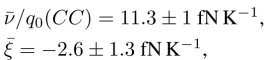
and for mixture 2:
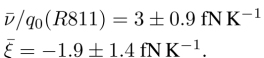
These measurements show that the value of the measured Leslie coefficient ![]() (or of the ratio
(or of the ratio ![]() /q0) depends on the chiral molecules, whereas the value of
/q0) depends on the chiral molecules, whereas the value of ![]() is the same for the two mixtures within the experimental errors. This is expected because
is the same for the two mixtures within the experimental errors. This is expected because ![]() is a nematic-like thermomechanical coefficient that should essentially depend on the LC used, here the CCN-37. It must be emphasized that
is a nematic-like thermomechanical coefficient that should essentially depend on the LC used, here the CCN-37. It must be emphasized that ![]() is only 3.8 times smaller in the mixture with R811, than in the mixture with the CC, although the concentration of R811 is 18 times smaller than that of CC. This means that the Leslie effect is 18/3.8 = 4.7 times stronger with the R811 than with the CC at equal concentrations. In other words, the LRP of the R811 is 4.7 times larger than the LRP of the CC, although the HTP of the R811 is 18 times larger than that of the CC. This again shows that the HTP and the LRP do not have the same origin, with the former corresponding to an equilibrium property, while the second is dynamic in nature.
is only 3.8 times smaller in the mixture with R811, than in the mixture with the CC, although the concentration of R811 is 18 times smaller than that of CC. This means that the Leslie effect is 18/3.8 = 4.7 times stronger with the R811 than with the CC at equal concentrations. In other words, the LRP of the R811 is 4.7 times larger than the LRP of the CC, although the HTP of the R811 is 18 times larger than that of the CC. This again shows that the HTP and the LRP do not have the same origin, with the former corresponding to an equilibrium property, while the second is dynamic in nature.
![]()
These results also show that in diluted mixtures ν and ![]() are of the same order of magnitude. This contrasts with the situation in compensated mixtures, in which the macroscopic term
are of the same order of magnitude. This contrasts with the situation in compensated mixtures, in which the macroscopic term ![]() must be negligible with respect to ν, since it must be of the same order of magnitude as in diluted mixtures. This confirms our suspicion that
must be negligible with respect to ν, since it must be of the same order of magnitude as in diluted mixtures. This confirms our suspicion that ![]() ≈ ν in the compensated mixtures studied before.
≈ ν in the compensated mixtures studied before.
Last but not least, we see that the experimental value of ξ, obtained from the previous value of ![]() by assuming that ξ = ξ2 = ξ3 = ξ4, is of the order of -15 fN/K, which is about 103 times smaller in absolute value than the value given by Akopyan and Zel’dovich in their theoretical paper (according to Akopyan and Zel’dovich (1984), ξ ∼ 10−11 N/K).
by assuming that ξ = ξ2 = ξ3 = ξ4, is of the order of -15 fN/K, which is about 103 times smaller in absolute value than the value given by Akopyan and Zel’dovich in their theoretical paper (according to Akopyan and Zel’dovich (1984), ξ ∼ 10−11 N/K).
3.4.4. Drift of cholesteric fingers under homeotropic anchoring
It is well known that the helical structure of a cholesteric LC is frustrated in a homeotropic sample, and all the more so, the sample is thin (Brehm et al. 1974). In usual cholesterics, this frustration leads to the complete unwinding of the helix when the sample thickness d is smaller than a critical thickness dc of the order of P. In this case, the director is perpendicular to the glass plates everywhere, forming a homeotropic nematic phase. By contrast, a fingerprint texture forms when d > dc. This texture is composed of cholesteric fingers (CF), which are typically separated from one another by homeotropic nematics when dc < d < 1.2dc and adhere to each other when d > 1.2dc. Finally, isolated fingers can coexist with the homeotropic nematic when d = dc. In this section, we analyze the behavior of these isolated fingers when they are subjected to a temperature gradient. In practice, several types of fingers may form in the samples, referred as to CF1, CF2, CF3 and CF4 in literature (for a review, see Oswald et al. (2000), Oswald and Pieranski (2005) and Smalyukh et al. (2005)). In the following, we focus on the CF1s, which are the only ones in which the director field is continuous everywhere (Press and Arrott 1976), and we show that they can drift and form spirals under the action of the temperature gradient (Oswald and Dequidt 2008c).
3.4.4.1. Theoretical predictions
The director field inside of a CF1 is shown in Figure 3.18. It can be numerically calculated by the minimization of the elastic energy. On this topic, we emphasize the important role of the elastic anisotropy, demonstrated for the first time in Lequeux et al. (1989). Indeed, isolated CF1s only form if the transition nematic→fingers is of the first order, which requires the elastic anisotropy to be large enough, according to the diagram shown in Figure 3.19 (Ribière et al. 1991). This is the case in most LCs, including those used in this work, in which K3 is larger than K1 and K2 (see Table 3.2, for instance).
Gil and Thiberge were the first (Gil and Thiberge 1997) to propose that a Leslie-like electromechanical effect could be responsible for the of the CF1s when they are subjected to a DC electric field (Gilli and Gil 1994). We know today that this drift is not due to this effect, but to a coupling between the director field and the flows associated with the motion of flexoelectric polarization charges (Tarasov et al. 2003). However, the Gil and Thiberge model applies the thermomechanical case by replacing the electric field by the temperature gradient. In this model, the authors solve the torque equation in a perturbative way, for small values of the field, by using a Melnikov-type analysis. It turns out that this method is complicated and not general as it neglects the temperature variations of the material constants. For this reason, we propose another method (Dequidt 2008; Dequidt et al. 2016), which is completely general and easier to understand.

Figure 3.18. Director field inside of a CF1 when q0 > 0 (right-handed cholesteric). The “nail representation” has been used to represent the director field. Tilted molecules are represented by nails, proportional in length to the director projection in the plane of the drawing

Figure 3.19. Nature of the frustration transition in the plane of the anisotropy parameters K12 = K1/K2 and K32 = K3/K2. Reprinted from Phys. Rev. A, 44, 8198 (1991), Copyright 1999, American Physical Society
The starting point of the calculation consists of noticing that the total energy of a finger (including the elastic energy ![]() and the anchoring energy on the glass plates
and the anchoring energy on the glass plates ![]() ) does not change in time when the finger drifts perpendicularly to its long axis at constant velocity V. This condition reads
) does not change in time when the finger drifts perpendicularly to its long axis at constant velocity V. This condition reads
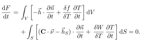
Replacing ![]() in this equation by their expressions given in equations [3.9] and [3.12] yields
in this equation by their expressions given in equations [3.9] and [3.12] yields

If the finger propagates along the y-axis with velocity V, then ![]() and
and ![]() with
with
where V(TM) is the drift velocity due to thermomechanical cross-coupling and V(T) is the drift velocity due to the variation of the free energy with temperature:
[3.90]
with
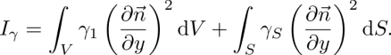
Formula [3.90] shows that, in addition to the thermomechanical terms, the variation in temperature of both the elastic constants and the anchoring energy can lead to a drift18. An important point is that this drift is due to the transverse gradient ![]() The latter exists because of the anisotropy of the thermal conductivity of the LC.
The latter exists because of the anisotropy of the thermal conductivity of the LC.
We conclude this section by giving a simplified expression of V(TM). It is obtained by neglecting the surface viscosity γS and the anisotropy of thermal conductivity, which is the same as assuming that the temperature gradient is little different from the average gradient ![]() . If G is not too large (linear regime), the spatial variations of the material constants can also be neglected, and the director
. If G is not too large (linear regime), the spatial variations of the material constants can also be neglected, and the director ![]() can be replaced by the equilibrium solution
can be replaced by the equilibrium solution ![]() (linear regime). Under these assumptions, V(TM) can be calculated by using the expressions of
(linear regime). Under these assumptions, V(TM) can be calculated by using the expressions of ![]() and
and ![]() given in equations [3.22] and [3.24]:
given in equations [3.22] and [3.24]:
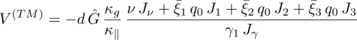
where the dimensionless integrals Ji are defined by

This formula generalizes a formula already given in Gil and Thiberge (1997); Oswald and Dequidt (2008c), where the thermomechanical coefficients ![]() were neglected 19.
were neglected 19.
Several remarks are in order as follows. First, we note that q0d in integrals J1, J2 and J3 must be equal to q0dc to observe isolated fingers. As a result, these integrals only depend on the elastic anisotropy and are independent of the sample thickness.
Another important point is that the integrals Jν,Jγ and Ji (1 = 1 − 3) do not change sign when q0 changes sign. As a result, the AZ contribution to v(TM) must change sign when q0 changes sign, contrary to the Leslie contribution, the sign of which is given by the sign of ν (independent of q0). Finally, we note that V(T) also changes sign when q0 changes sign, since ![]() changes sign when q0 changes sign.
changes sign when q0 changes sign.
3.4.4.2. Experimental results
The drift of cholesteric fingers subjected to a temperature gradient has been observed in two very different systems: in a compensated mixture close to the compensation temperature and in a diluted cholesteric mixture close to a cholesteric-smectic A phase transition. In the first case, we will show that the drift is due to the Leslie thermomechanical coupling, while it is likely due to the divergence of the twist and bend constants in the second case.
3.4.4.2.1. Drift close to a compensation temperature
The compensated mixtures are particularly well suited to observe the drift of CF1s for three reasons. First, the pitch changes with temperature. As a result, it is easy to fulfill the condition d = dc for a large range of thicknesses by just changing the sample temperature. Second, the Leslie coefficient is large, which is essential to observe a drift. Third, the experiment can be performed at two temperatures T1 < Tc and T2 > Tc, on either side of the compensation temperature, which allows the testing of the role of the sign of q0 on the drift velocity.
In practice, short segments of CF1 form in homeotropic samples when d = dc. These segments have two necessarily different ends because of the absence of mirror symmetry in a cholesteric. One of them is rounded, marked with the minus sign on the pictures, while the other is pointed, marked with the plus sign20. Under the action of a temperature gradient, these segments drift perpendicularly to their axes, as shown in Figure 3.20. In this figure, the x-axis is oriented from the pointed tip to the rounded tip. With this choice, the experiments with the mixture 8OCB + 50 wt% CC show that V is positive (negative) when ΔT > 0 (ΔT < 0) at the two temperatures T1 and T2, independent of the sign of q0. The velocity is also found proportional to the temperature gradient (linear regime) and proportional to d, as shown in Figure 3.21. These results – particularly the fact that V does not change sign at Tc – show that the drift is mainly due to the Leslie thermomechanical coupling. This interpretation was confirmed by numerically calculating the constant from which a value of ν was found by taking ![]() ν ≈ 1.3 × 10⁻⁷ kg K−1 s−2 at Tc. This value is very close to the values previously given, confirming that the drift is mainly due to the Leslie thermomechanical coupling.
ν ≈ 1.3 × 10⁻⁷ kg K−1 s−2 at Tc. This value is very close to the values previously given, confirming that the drift is mainly due to the Leslie thermomechanical coupling.
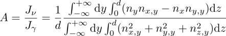
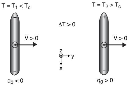
Figure 3.20. Drift direction of CF1 segments observed in homeotropic samples of the mixture 8OCB + 50 wt% CC on both sides of the compensation temperature. Although q0 changes sign, the drift direction is always the same. Drawing inspired by Oswald and Dequidt (2008c)

Figure 3.21. (a) Drift velocity as a function of the temperature difference ΔT , measured in a sample of thickness d = 10 μm at temperature T2 > Tc. (b) Ratio of the drift velocity over the temperature difference times the sample thickness as a function of the equilibrium twist or the temperature. □, d = 10 μm; ©, d = 25 μm; , d = 40 μm. Reprinted from Oswald and Dequidt (2008c), Copyright 2008, American Physical Society
It should also be noted that isolated CF1s can be stabilized by the application of an AC electric field, when the sample temperature is larger than T2. In this case, the pitch becomes smaller than the thickness and the CF1s become unstable, growing from their ends while undulating until they invade the whole sample. The only way to stabilize the fingers again is to impose an electric field to favor the homeotropic nematic with respect to the fingers. The equilibrium is reached for a voltage denoted by V2 in literature. Of course, the larger the temperature above T2, the larger V2 is and the thinner the CF1s are, whose width always remains close to 3.5P (Ribière and Oswald 1990). It is then possible to impose a temperature gradient to the fingers and to measure their drift velocity. Such measurements were performed in a 15-μm-thick sample of the mixture 8OCB + 50 wt% CC. The results, reported in Figure 3.22, show that the drift velocity strongly decreases when the temperature and the electric fields increase. This effect is expected since A must be roughly proportional to the width of the finger according to equation [3.94], a quantity close to 3.5P that strongly decreases when the temperature increases.
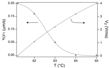
Figure 3.22. Drift velocity of the CF1s and coexistence voltage V2 as a function of temperature above the compensation temperature. Mixture 8OCB + 50 wt% CC, d = 15 μm, T2 = 61◦C and ΔT = 30◦C. Reprinted from Oswald (2008) with the permission of Taylor & Francis
We conclude this section by noting that the isolated segments of CF1 always destabilize in time by forming spirals. This evolution is inevitable (as shown in Pirkl and Oswald (1996); Oswald et al. (2000)) and is akin to what is observed with wave fronts in weakly excitable two-dimensional media (Mikhailov et al. 1994). Figure 3.23 shows two single and two triple spirals observed above and below the compensation temperature. The reader will note that these two types of spirals do not rotate in the same sense when T > Tc and ΔT > 0. This is due to the fact that the rounded tips lie in the center of the single spirals and on the outer border of the triple spirals, showing that the fingers are oriented in opposite directions in these two types of spirals. These images also show that far from their center, the spirals tend to
Archimedian spirals of an equation in polar coordinates
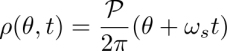
where ![]() is the pitch of the spiral and ωs is its angular rotation velocity related to the drift velocity by the relation
is the pitch of the spiral and ωs is its angular rotation velocity related to the drift velocity by the relation


Figure 3.23. (a-b) Two single spirals rotating in the same direction observed in a 25 μm-thick sample at T = T1 = 56.4◦C (a) and T = T2 = 58.9◦C (b) when ΔT = 47.2◦C; (c-d) Two triple spirals rotating in opposite directions at T = T2 = 60.8◦C under a temperature difference ΔT = 36.8◦C (c) and ΔT = −43.6◦C in a 10-μm-thick sample. Mixture 8OCB + 50 wt% CC. Reprinted from Oswald and Dequidt (2008c), Copyright 2008, American Physical Society
This equation is general and gives the product ωs![]() . On the other hand, ωs (and, thus,
. On the other hand, ωs (and, thus, ![]() ) depends on the anchoring conditions of the spiral at the center, which may change from one spiral to another.
) depends on the anchoring conditions of the spiral at the center, which may change from one spiral to another.
3.4.4.2.2. Drift close to a cholesteric-smectic A phase transition
The same experiment was conducted in the diluted mixture 8OCB + 1.14 wt% R811 (Oswald 2008). In this mixture, the Leslie coefficient is much smaller than in the compensated mixture because of the small concentration of chiral molecules and the Akopyan and Zel’dovich terms entering into the expression [3.92] of the drift velocity, which are not larger than the Leslie term according to our previous estimate of the ¯i. As a result, these fingers should not drift in a visible way. This is indeed what we have found experimentally, except very close to the smectic A phase transition where the CF1 spontaneously formed spirals, as shown in Figure 3.24. This result is very surprising as we know that the viscosity γ1 diverges at the smectic A-to-nematic phase transition (de Gennes and Prost 1995; Oswald and Pieranski 2006). One possibility to explain this observation with the “classical” thermomechanical model would be that the Leslie coefficient diverges faster than γ1. To test this idea, measurements in the Leslie geometry were performed with the mixture 8CB + 1 wt% R811. It was found that the rotation velocity continuously decreases when approaching the smectic A phase, which clearly indicates that ![]() does not diverge but remains approximately constant (Oswald 2016). These results show that this drift is not due to the classical thermomechanical coupling, but rather to the other mechanism described above, coming from the temperature variations of the free energy. The corresponding drift velocity V(T) is given in equation [3.90]. This expression simplifies if the anchoring energy is very large and if the glass conductivity is much larger than that of the LC. In these limits,
does not diverge but remains approximately constant (Oswald 2016). These results show that this drift is not due to the classical thermomechanical coupling, but rather to the other mechanism described above, coming from the temperature variations of the free energy. The corresponding drift velocity V(T) is given in equation [3.90]. This expression simplifies if the anchoring energy is very large and if the glass conductivity is much larger than that of the LC. In these limits, ![]() both tend to 0 on the glass plates, leading to
both tend to 0 on the glass plates, leading to
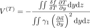
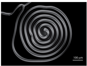
Figure 3.24. Spiral of CF1 observed between crossed polarizers close to the smectic phase. Mixture 8OCB + 1.14 wt% R811. ΔT = −40◦C and d = 15 μm. In this experiment, an electric field was applied to stabilize the finger (V = 1.98 Vrms and f = 1 kHz). Reproduced from Oswald (2008) with the kind permission of Taylor & Francis
This formula shows that the drift velocity is proportional to the horizontal temperature gradient. By denoting the temperature at the bottom of the glass plate by T0, it can be shown by using the heat equation, and by setting ![]() where g is the solution of
where g is the solution of

with g = 0 at z = 0 and z = d. This shows that the horizontal gradient is proportional to ![]() and is different from 0 as long as κa
and is different from 0 as long as κa ![]() 0. Due to this temperature gradient, one side of the finger is colder than the other21. For this reason, the finger tends to drift toward its hotter side to minimize its elastic energy. To some extent, one can say that the finger surfs on a heat wave that it creates itself. From the previous expression, one can estimate the order of magnitude of the drift velocity by orienting the finger in the same way as in Figure 3.20. This gives, within a numerical factor impossible to estimate by hand (Dequidt et al. 2016):
0. Due to this temperature gradient, one side of the finger is colder than the other21. For this reason, the finger tends to drift toward its hotter side to minimize its elastic energy. To some extent, one can say that the finger surfs on a heat wave that it creates itself. From the previous expression, one can estimate the order of magnitude of the drift velocity by orienting the finger in the same way as in Figure 3.20. This gives, within a numerical factor impossible to estimate by hand (Dequidt et al. 2016):

where K is a combination of the elastic constants that diverges at the transition. This mechanism could explain the formation of spirals close to the transition. However, numerical simulations would be important to confirm this interpretation.
We end this section by mentioning the existence of another thermomechanical effect observed during the growth of cholesteric fingers. As we mentioned before, CF1s grow from their ends while undulating when the confinement ratio is too large, typically more than 1, and the applied voltage (if any) is less than V2. We have observed that during the growth, the ends of the fingers move at constant speed in a straight line when no temperature gradient is applied. By contrast, they follow circular trajectories when a temperature gradient is applied, the radius of which decreases when the temperature gradient increases. An example is shown in Figure 3.25. This phenomenon is observed at all temperature, but has not yet been explained.
3.5. The thermohydrodynamical effect
In our experiments, we did not observe visible flows and, for this reason, we neglected them in our previous analyses. This is fully justified in the experiments on the Leslie geometry, when the director field is not distorted in the plane of the sample because, in that case, the solution to the full problem is ![]() = 0 everywhere, when
= 0 everywhere, when ![]() = 0 on the boundaries of the LC domain. By contrast, flows should be present in the Leslie geometry close to the disclination lines, even if we have not yet detected them. However, the fact that we measured the same director rotation velocity in the homogeneous regions and close to the disclination lines clearly indicates that hydrodynamic flows interfere very little with the thermomechanical effect. In the following, we propose a method to measure the TH Leslie coefficient μ in a compensated mixture. We will then return to the mixed geometry, which has been used to estimate the TH Akopyan and Zel’dovich terms ξi (i = 5 − 12). Two experiments will be described, that both led to surprisingly large values for these coefficients.
= 0 on the boundaries of the LC domain. By contrast, flows should be present in the Leslie geometry close to the disclination lines, even if we have not yet detected them. However, the fact that we measured the same director rotation velocity in the homogeneous regions and close to the disclination lines clearly indicates that hydrodynamic flows interfere very little with the thermomechanical effect. In the following, we propose a method to measure the TH Leslie coefficient μ in a compensated mixture. We will then return to the mixed geometry, which has been used to estimate the TH Akopyan and Zel’dovich terms ξi (i = 5 − 12). Two experiments will be described, that both led to surprisingly large values for these coefficients.

Figure 3.25. Growth of a CF1 in the homeotropic nematic. The dashed lines show the trajectory of the rounded tip when ΔT = 0 (a), ΔT = 40◦C (b) and ΔT = −40◦C. The polarizer and analyzer are at 45◦ relative to each other. Mixture 8OCB + 1.14 wt% R811; d = 10 μm, T = 50◦C, V = 2 Vrms < V2 = 4 Vrms. Reproduced from Oswald (2008) with the kind permission of Taylor & Francis
3.5.1. A proposal for measuring the TH Leslie coefficient μ: theoretical prediction
We have seen how to measure the TM Leslie coefficient ν in a compensated cholesteric at the compensation temperature. A question that arises is whether it is possible to measure the associated TH term μ. We already mentioned that this term does not play any role in the Leslie geometry when the director field is not distorted in the plane of the sample. In this section, we show that the situation is different around a +1 disclination line. To simplify the problem, we assume that the director cannot rotate on the plates and in the bulk and is either oriented in a circular configuration (Figure 3.26(a)) or in a radial configuration (Figure 3.26(b)). Experimentally the circular configuration can be obtained by treating one plate with the polymercaptan to obtain a sliding planar anchoring and the other with a polyimide for planar alignment. The latter is then briefly pressed against a piece of velvet fabric kept in continuous rotation. In this way, the surface easy axis has the desired +1 circular geometry, which leads to the configuration described in Figure 3.26(a), after the sample has been filled with the LC. It is then enough to let the sample rest for 1 day to memorize the circular anchoring on the plate treated with the polymercaptan and block the rotation of the director on this plate. This method cannot be used to prepare the radial configuration. In that case, a photoalignment technique must be used, such as the one described in Slussarenko et al. (2011), to which we refer for more details.
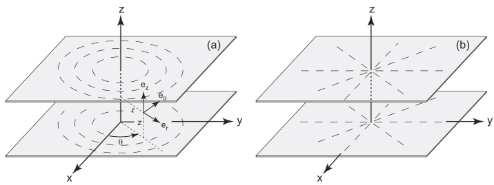
Figure 3.26. Circular (a) and radial (b) configurations and system of polar coordinates (r, θ, z)
To calculate the flow around the +1 disclination line, we solved in polar coordinates (r, θ, z) (see Figure 3.26(a)) the momentum equation ![]() · σ = 0, where σ ≡ −P
· σ = 0, where σ ≡ −P ![]() + σ(eq) + σ(neq). In these equations, P is the pressure given by the incompressibility condition
+ σ(eq) + σ(neq). In these equations, P is the pressure given by the incompressibility condition ![]() By assuming that the director field is imposed by the anchoring conditions, we have
By assuming that the director field is imposed by the anchoring conditions, we have ![]() = (0, 1, 0) in the circular geometry and
= (0, 1, 0) in the circular geometry and ![]() in the radial geometry. As a result,
in the radial geometry. As a result, ![]() · σ(eq) = 0 and the momentum equation becomes
· σ(eq) = 0 and the momentum equation becomes ![]() ), where σ(v) is the viscous stress tensor given in equation [3.21] and σ(L) the Leslie stress tensor given in equation [3.22]. To further simplify the problem, we assume that q0 = 0 (cholesteric at the compensation temperature) and that the viscosity, TM and TH coefficients αi, ν and μ are constant within the sample thickness.
), where σ(v) is the viscous stress tensor given in equation [3.21] and σ(L) the Leslie stress tensor given in equation [3.22]. To further simplify the problem, we assume that q0 = 0 (cholesteric at the compensation temperature) and that the viscosity, TM and TH coefficients αi, ν and μ are constant within the sample thickness.
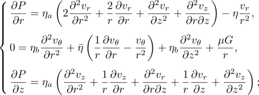
and in the radial geometry as:
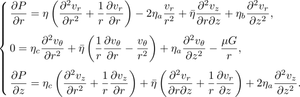
In these expressions ![]() and
and ![]() are the three Miesowicz viscosities (de Gennes and Prost 1995; Oswald and Pieranski 2005) and we set
are the three Miesowicz viscosities (de Gennes and Prost 1995; Oswald and Pieranski 2005) and we set ![]() .
.
As for the incompressibility condition, it reduces to:

An important point to note here is that only the TH Leslie coefficient μ enters into the problem. These equations immediately show that the solution is of the type vr = vz = 0 with P = constant. As for the orthoradial component vθ(r, z), it is given by solving the second equation in [3.100] for the circular configuration and in [3.101] for the radial configuration with the boundary conditions vθ(rc,z) = vθ(R, z) = vθ(r, 0) = vθ(r, d) = 0. Here, rc denotes the core radius of the disclination, R is its outer radius and d is the sample thickness. These equations can be solved with Mathematica. The resolution shows that a circular flow develops locally around the core of the disclination line (Figure 3.27). The velocity is proportional to μ and the temperature gradient G and passes through a maximum proportional to d at z = d/2 and r ≈ d/2. The senses of rotation are opposite in the circular and radial configurations. Finally, the velocity decreases at long distance (r > d)as
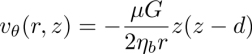
in the circular geometry and as

in the radial geometry.
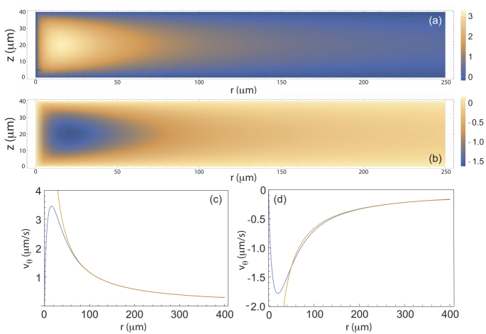
Figure 3.27. (a, b) vθ-amplitude in the radial plane (r, z) and (c,d) vθ-profile along the r-axis at z = d/2. The blue curves have been calculated numerically and the yellow curves represent the asymptotic solutions given in equations [3.103] and [3.104]. (a and c) Circular geometry and (b and d) radial geometry
The orders of magnitude of the velocity fields in both configurations are shown in Figure 3.27. Simulations were performed by taking d = 40 μm, rc = 0.05 μm, R = 400 μm, G = 7 104 K/m (ΔT = 40◦C), ηa = 0.042 Pa s, ηb = 0.024 Pa s, ηc = 0.1 Pa s, α1 = 0, γ1 = 0.075 Pa s and by assuming that μ ≈ ν = 2 10−7 kg s−2 K−1. With these values, ![]() in the circular geometry and
in the circular geometry and ![]() in the radial configuration. In practice, such flow should be experimentally detectable.
in the radial configuration. In practice, such flow should be experimentally detectable.
3.5.2. About the measurement of the TH Akopyan and Zel’dovich coefficients
3.5.2.1. Principle of the measurement
The basic idea for measuring the order of magnitude of the TH coefficients ξi (i = 5 − 12) in a nematic phase was already given in the seminal paper by Akopyan and Zel’dovich (1984). Indeed, these authors note from the beginning of their paper that a flow should be induced by a temperature gradient in a mixed sample treated for planar unidirectional anchoring on one plate and homeotropic anchoring on the opposite plate (Figure 3.28(a)). The order of magnitude of the velocity v can be easily found by solving the momentum equation ![]() This equation considerably simplifies if one assumes that
This equation considerably simplifies if one assumes that ![]() in the (x, y, z) reference frame, with
in the (x, y, z) reference frame, with ![]() 22; (2) the temperature gradient is constant, equal to G 23 and (3) the material constants do not change with temperature in the sample thickness. By using the simplified expression of σ(AZ) given in equation [3.31], and by further assuming that the nematic phase behaves viscously as an isotropic liquid of viscosity η, we obtain:
22; (2) the temperature gradient is constant, equal to G 23 and (3) the material constants do not change with temperature in the sample thickness. By using the simplified expression of σ(AZ) given in equation [3.31], and by further assuming that the nematic phase behaves viscously as an isotropic liquid of viscosity η, we obtain:
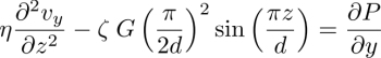

Figure 3.28. Mixed planar-homeotropic geometry. In (a), the anchoring is planar unidirectional on the top plate and in (b), it is planar circular
The reader will note that the TM term in ξ and the TH terms in ![]() and
and ![]() do not enter into this equation when α varies linearly with z.
do not enter into this equation when α varies linearly with z.
If the nematic phase is free to flow along the x-axis, then P = constant and the solution reads
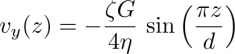
As expected, the velocity is maximum in the middle of the sample and vanishes on the two glass plates. One will note that the velocity at z = d/2 is independent of the sample thickness because the TH and viscous stresses both vary as 1/d.
This calculation assumes that the LC can flow freely along the x-axis, which is difficult to realize in practice. Indeed, the flow disappears as long as the LC is in contact with an obstacle (for instance, one of the spacers used to control the sample thickness). In that case, the TH stress is equilibrated by a pressure gradient and no flow occurs.
To avoid this difficulty, Akopyan and coworkers proposed to perform the experiment in a sample treated for planar circular anchoring on one plate and homeotropic anchoring on the opposite plate (Akopyan et al. 1999, 2001, 2004). This geometry is represented in Figure 3.28(b).
3.5.2.2. Theoretical predictions in the mixed planar-circular/homeotropic geometry
Because of the axial symmetry, calculations can be done in cylindrical coordinates by taking ![]() To write the equations, we used Mathematica and assumed that (1) the director field is given by
To write the equations, we used Mathematica and assumed that (1) the director field is given by ![]() with
with ![]() in the referential frame
in the referential frame ![]() (2) G is constant; (3) the material constants are independent of temperature and (4) the AZ stress tensor is given by the simplified expression [3.31]. However, we used the full expression of the viscous stress tensor given in equation [3.21], in which we made
(2) G is constant; (3) the material constants are independent of temperature and (4) the AZ stress tensor is given by the simplified expression [3.31]. However, we used the full expression of the viscous stress tensor given in equation [3.21], in which we made ![]() because this term is usually very small in nematics (de Gennes and Prost 1995; Oswald and Pieranski 2005). In spite of the approximations, the equations are very long and will not be given here. We will just focus on the equation in
because this term is usually very small in nematics (de Gennes and Prost 1995; Oswald and Pieranski 2005). In spite of the approximations, the equations are very long and will not be given here. We will just focus on the equation in ![]() far from the core of the disclination (typically for
far from the core of the disclination (typically for ![]() ). In this region, vr and vz tend to 0, and so can be neglected as well as the terms in
). In this region, vr and vz tend to 0, and so can be neglected as well as the terms in ![]() and
and ![]() which gives
which gives
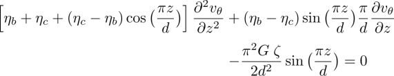
The solution to this equation reads
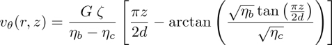
As expected, it can be checked that in the limit ηb → ηc = η, this equation gives back the result of equation [3.106]. This equation shows that far from the core of the disclination (in practice at distance r > d), a circular flow develops with a velocity in the center of the sample at z = d/2, given by
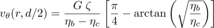
The reader will note that, as under unidirectional planar anchoring, the constants ξ, ζ’ and ζ” do not enter into the solution far from the core of the disclination. This is not the case close to the core where the two terms in ζ’ and ζ” are important. On the other hand, the TM term in ξ vanishes everywhere if the angle between the director and the z-axis varies linearly with z, as assumed in this calculation. The numerical solution to the full equations is shown in Figure 3.29 and is compared to the approximate solution given in equation [3.109]. In this simulation, we chose the same values for the material constants as in Figure 3.27, and we took ζ = ζ’ = ζ” = 10−12 NK−1.
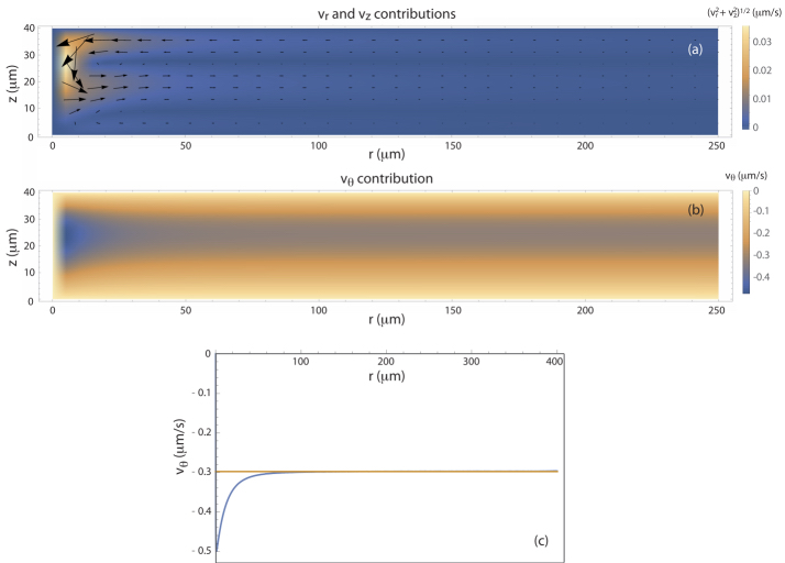
Figure 3.29. Velocity field in the planar-circular/homeotropic geometry. (a)  -amplitude and (b) vθ-amplitude in the (r, z)-plane. The arrows represent the projection of velocity field in the (r, z)-plane. (c) vθ as a function of r at z = d/2. The yellow curves represent the asymptotic solutions given in equation [3.109]
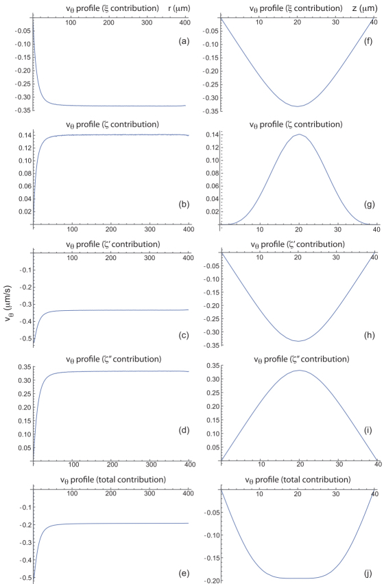
Figure 3.30. Orthoradial component of the velocity vθ as a function of r at z = d/2 = 20 μm (a–e) and as a function of z at d = 100 μm when θm = 1 rad (f–j). (a and f) ξ  0 and ζ = ζ = ζ” = 0; (b and g) ζ = 0 and ξ = ζ = ζ” = 0; (c and h) ζ
  0 and ξ = ζ = ζ” = 0; (d and i) ζ”
  0 and ξ = ζ = ζ = 0; (e, j), ξ = ζ = ζ = ζ”
  0
0
As expected, these calculations confirm that a circular flow develops at distance r > d of the core of the disclination. An important point is that the velocity in the middle of the sample is proportional to G and ζ and is independent of r. The latter result contrasts with the numerical simulation of Akopyan et al. (2004), who found that the maximal velocity along z, ![]() was proportional to r. We think that this result is wrong as we found a similar result to ours by numerically solving their own equations with Mathematica.
was proportional to r. We think that this result is wrong as we found a similar result to ours by numerically solving their own equations with Mathematica.
We note that another variant of the experiment has been proposed in Akopyan et al. (2001). It consists of destabilizing, with an AC electric field, a sample treated for the circular configuration. If the applied voltage V is larger than the Fréedericksz critical voltage Vc, the director field distorts and reads in polar coordinates in the form ![]() with
with ![]() and
and ![]() provided that V < 1.3 Vc. The same calculations as before shows that a circular flow develops around the core of the disclination. At distance r > d, the only non-zero component of the velocity is vθ. This component depends on all of the TH coefficients ζ, ζ’ and ζ”, but also on the TM coefficient ξ, as shown in Figure 3.30. In this figure, we plotted vθ(r, d/2) as a function of r and vθ(r, z) calculated at r = 100 μm as a function of z for each contribution ξ, ζ, ζ’ and ζ” and for the total contribution. In this calculation, we assumed that ξ = ζ = ζ’ = ζ” = 10−12 N/K24 and we took θm = 0.8 rad and the same values as before for the other parameters. These calculations show that all of the terms contribute in a similar way and lead to typical velocities of the order of 0.15 − 0.3 μm/s.
provided that V < 1.3 Vc. The same calculations as before shows that a circular flow develops around the core of the disclination. At distance r > d, the only non-zero component of the velocity is vθ. This component depends on all of the TH coefficients ζ, ζ’ and ζ”, but also on the TM coefficient ξ, as shown in Figure 3.30. In this figure, we plotted vθ(r, d/2) as a function of r and vθ(r, z) calculated at r = 100 μm as a function of z for each contribution ξ, ζ, ζ’ and ζ” and for the total contribution. In this calculation, we assumed that ξ = ζ = ζ’ = ζ” = 10−12 N/K24 and we took θm = 0.8 rad and the same values as before for the other parameters. These calculations show that all of the terms contribute in a similar way and lead to typical velocities of the order of 0.15 − 0.3 μm/s.
3.5.2.3. Experimental results
The experiment was performed by Akopyan and coworkers in the two mixed geometries depicted in Figure 3.29. In the two cases, the authors observe a flow with a maximal velocity proportional to the temperature gradient and of the order of 1 μm/s for G ≈ 1.4 105 K/m (Akopyan et al. 1997, 1999). This is in favor of a thermohydrodynamical effect with coefficients ζ, ζ’ or ζ” of the order of 10−12 N/K, which is the value we have taken in our previous numerical simulations. However, the authors observe in the circular geometry of Figure 3.28 that the velocity increases linearly with the radius (see Figure 4 in Akopyan et al. (2001)), which is incompatible with our own numerical simulations. This is a real problem for which we have no solution to propose for the moment. In addition, these results suggest that the thermohydrodynamical coefficients ζ, ζ’ or ζ” are much larger than the thermomechanical coefficient ξ in the order of 10−15 N/K, according to our experiments. This is surprising and for this we do not have any explanation. Note that an even larger value was given by Lavrentovich and Nastishin (1987) to explain the flows observed in flattened droplets deposited on a bath of glycerol and submitted to a temperature gradient25. The problem in this experiment is the presence of the Marangoni effects that can distort the measurements. The same problem occurs in the experiment by Choi and Takezoe (2016), showing the formation at the place where a laser beam is focused on a localized circular flow in a homeotropically oriented nematic layer with a free surface. In the paper by Choi and Takezoe, this effect is interpreted to be due to a Marangoni effect, but an alternative explanation was proposed by Zakharov and Maslennikov (2019) in terms of the thermohydrodynamical effect, provided the ζ-coefficients are large enough.
3.6. Conclusions and perspectives
Until recently, it was thought that the main experimental evidence of the Leslie thermomechanical effect was the rotation of cholesteric droplets subjected to a temperature gradient, the so-called Lehmann effect. This standpoint is mistaken in our opinion, because other mechanisms exist – more efficient than the Leslie effect – to explain the Lehmann effect (for a review, see (Oswald et al. 2019a)). This is the reason why in this chapter we distinguished the Lehmann effect discovered experimentally by Lehmann in 1900, from the thermomechanical effect discovered theoretically by Leslie in 1968. If the latter does not fully explain the Lehmann effect, it nonetheless exists and is clearly measurable in cholesterics. We have shown this result by describing the static Éber and Jánossy experiment and the dynamic experiments on the rotation of the TICs under sliding anchoring. An important point to note is that the Leslie effect still exists at the compensation temperature of a cholesteric phase, at which the helix is unwound.
The situation is more complex for the thermomechanical effect described by Akopyan and Zel’dovich in distorted nematics and cholesterics. These terms are associated with macroscopic distortions of the director field and are more difficult to measure. The comparative experiments with two different types of TICs have nonetheless proven their existence and have allowed us to estimate their order of magnitude.
By contrast, the situation is much more confusing concerning the thermohydrodynamical effects predicted in both cholesterics and deformed nematics. At the moment, there is no experimental evidence of the Leslie thermohydrodynamical effect in cholesterics, but we proposed an experiment to evidence it at the compensation temperature. Concerning the thermohydrodynamical effect in a deformed nematic, only two experiments have been conducted, the first by Lavrentovish and Nastishin and the second by Akopyan and collaborators. In the former, a droplet is deposited at the surface of a bath of glycerol. The problem in this experiment is the presence of Marangoni effects that can distort the measurements. For this reason, we prefer the Akopyan experiment realized between two glass plates treated for homeotropic and circular planar anchoring, respectively. In this case, there are no Marangoni effects, which greatly simplifies the predictions. In this experiment, circular flows are indeed detected by Akopyan et al. but the radial profile of the orthoradial velocity measured experimentally does not match with theory, according to our calculations. For this reason, we have some reservations about the value of the thermohydrodynamical coefficients found by these authors. These doubts are reinforced by the fact that this order of magnitude is not compatible with the one of the thermomechanical coefficients we have found experimentally – if we agree that all of the coefficients must be of the same order of magnitude, which is perhaps not the case. An alternative explanation for this disagreement could be that the thermohydrodynamical flows – which we neglected in our calculations – couple and slow down the rotation of the director in the mixed geometry under sliding planar anchoring, leading us to strongly underestimate the thermomechanical coefficients. For these reasons, we think that the experiments in mixed geometry need to be reproduced for confirmation in the future, in particular in the circular configuration when the director is fixed or free to rotate. In the latter case, it would also be important to numerically solve the full equations to determine if the circular flow disturbs the rotation of the director.
It is clear that knowing the order of magnitude of the Akopyan and Zel’dovich coefficients would be important in the future to determine whether the thermohydrodynamical effect could be potentially useful for applications in microfluidics, as recently proposed by Zakharov and collaborators (Zakharov and Vakulenko 2009; Zakharov et al. 2010; Śliwa and Zakharov 2020). The same issue arises in nonlinear optics where the thermohydrodynamical effect could induce flows and director field distortions, leading to a nonlinear optical response of the LC when the samples are illuminated by laser beams. This was shown by Akopyan and collaborators (Akopyan et al. 2000; Hakobyan et al. 2012; Hakobyan 2015), Poursamad et al. (2010, 2015), and Krimer and Residori (2007), who predicted molecular reorientation at intensities substantially lower than that needed for optical Fréedericksz transition in a dye-doped nematic sample.
3.7. References
Akopyan, R.S. and Zel’dovich, B.Y. (1984). Thermomechanical effects in deformed nematics. Sov. Phys. JETP, 60, 953–958.
Akopyan, R.S., Alaverdyan, R.B., Santrosyan, E.A., Chilingaryan, Y.S. (1997). Thermomechanical effect in a hybrid-oriented nematic liquid crystal. Tech. Phys. Lett., 23, 690–691.
Akopyan, R.S., Alaverdyan, R.B., Santrosyan, E.A., Nersisyan, S.T., Chilingaryan, Y.S. (1999). Thermomechanical effect in a cylindrical-hybrid nematic liquid crystal. Tech. Phys. Lett., 25, 237–238.
Akopyan, R.S., Zel’dovich, B.Y., and Seferyan, H. (2004). Thermomechanical coupling in a cylindrical hybrid-aligned nematic liquid crystal. JETP, 99, 1039–1043.
Akopyan, P.C., Alaverdyan, R.B., Santrosyan, E.A., Chilingaryan, Y.S. (2000). Photoinduced thermomechanical effect in homogeneous nematics. Quantum Elec., 30, 653–654.
Akopyan, R.S., Alaverdian, R.B., Santrosian, E.A., Chilingarian, Y.S. (2001). Thermomechanical effects in the nematic liquid crystals. J. Appl. Phys., 90, 3371–3376.
Baudry, J., Brazovskaia, M., Cek, L.L., Oswald, P., Pirkl, S. (1996). Arch-texture in cholesteric liquid crystals. Europhys. Lett., 21, 893–901.
Brand, H.R. and Pleiner, H. (1988). New theoretical effects for the Lehmann effect in cholesteric liquid crystals. Phys. Rev. A, 37, 2736.
Brehm, M., Finkelmann, H., Stegemeyer, H. (1974). Orientierung cholesterischer mesophasen an mit lecithin behandelten oberflächen. Ber. Bunsenges. Phys. Chem., 78, 883–886.
Casimir, H.B.G. (1945). On Onsagers principle of microscopic reversibility. Rev. Mod. Phys., 17, 343.
Choi, H. and Takezoe, H. (2016). Circular flow formation triggered by Marangoni convection in nematic liquid crystal films with a free surface. Soft Matter, 12, 481–485.
Daivis, P.J. and Evans, D.J. (1994). Non-equilibrium molecular dynamics calculation of thermal conductivity of flexible molecules: Butane. Mol. Phys., 81(6), 1289–1295.
Dauxois, T. and Peyrard, M. (2006). Physics of Solitons. Cambridge University Press, Cambridge.
Demenev, E.I., Pozdnyakov, G.A., Trashkeev, S.I. (2009). Nonlinear orientational interaction of a nematic liquid crystal with a heat flux. Techn. Phys. Lett., 35, 674–677.
Dequidt, A. (2008). Effet Lehmann dans les cristaux liquides cholestériques. PhD Thesis, University of Lyon, Ecole Normale Supérieure de Lyon.
Dequidt, A. and Oswald, P. (2007a). Does electric Lehmann effect exist in cholesteric liquid crystals? Eur. Phys. J. E, 25, 157.
Dequidt, A. and Oswald, P. (2007b). Lehmann effect in compensated cholesteric liquid crystals. Europhys. Lett., 80, 80.
Dequidt, A., ˙Nywociński, A., Oswald, P. (2008). Lehmann effect in compensated cholesteric liquid crystals: Experimental evidence with fixed and gliding boundary conditions. Eur. Phys. J. E, 25, 277.
Dequidt, A., Poy, G., Oswald, P. (2016). Generalized drift velocity of a cholesteric texture in a temperature gradient. Soft Matter, 12, 7529.
Dozov, I., Nobili, M., Durand, G. (1997). Fast bistable nematic display using monostable surface switching. Appl. Phys. Lett., 70, 1179.
Éber, N. and Jánossy, I. (1982). An experiment on the thermomechanical coupling in cholesterics. Mol. Cryst. Liq. Cryst. Lett., 72, 233.
Éber, N. and Jánossy, I. (1984). Thermomechanical coupling in compensated cholesterics. Mol. Cryst. Liq. Cryst. Lett., 102, 311.
Éber, N. and Jánossy, I. (1988). Note on “macroscopic description of compensated cholesteric and chiral smectic liquid crystals”. Mol. Cryst. Liq. Cryst. Lett., 5, 81.
Evans, D.J. and Murad, S. (1989). Thermal conductivity in molecular fluids. Molecular Physics, 68(6), 1219–1223.
Gay, J.G. and Berne, B.J. (1981). Modification of the overlap potential to mimic a linear sitesite potential. J. Chem. Phys., 74(6), 3316–3319.
de Gennes, P.G. and Prost, J. (1995). The Physics of Liquid Crystals. Clarendon Press, Oxford.
de Groot, S.R. and Mazur, P. (1962). Non-equilibrium Thermodynamics. North-Holland, Amsterdam.
Gil, L. and Thiberge, S. (1997). Heat-driven rotation in cholesteric droplets with a double twisted structure. J. Phys. II, 7, 1499.
Gilli, J.M. and Gil, L. (1994). Static and dynamic textures obtained under an electric field in the neighbourhood of the winding transition of a strongly confined cholesteric. Liq. Cryst., 17, 1–15.
Hakobyan, M.R. (2015). Laser induced thermomechanical effect in hybrid oriented liquid crystal. Proc. Yerevan State Univ., 3, 42–48.
Hakobyan, R.S., Hakobyan, M.R., Aleksanyan, A.K., Gevorgyan, G.S., Alaverdyan, R.B. (2012). Some light-induced orientational effects in nematic liquid crystals. J. Phys. Conference Series, 350, 012034.
Ito, F., Yoshioka, J., Tabe, Y. (2016). Heat-driven rotation in cholesteric droplets with a double twisted structure. J. Phys. Soc. Jpn, 85, 14601.
Krimer, D.O. and Residori, S. (2007). Thermomechanical effects in uniformly aligned dye-doped nematic liquid crystals. Eur. Phys. J. E, 23, 77–82.
Lavrentovich, O.D. and Nastishin, Y.A. (1987). A thermomechanical effect in deformed nematic liquid crystals. Ukr. Fiz. Zh. (Russ. Ed.), 32, 710–712.
Lehmann, O. (1900). Structur, system und magnetisches verhalten flüssiger krystalle und deren mischbarkeit mit festen. Ann. Phys., 307, 649.
Lequeux, F., Oswald, P., Bechhoefer, J. (1989). Influence of anisotropic elasticity on pattern formation in a cholesteric liquid crystal contained between two plates. Phys. Rev. A, 40, 3974–3982.
Leslie, F.M. (1968). Some constitutive equations for liquid crystals. Arch. Rational. Mech. Anal., 28, 265.
Lim, K.C. and Ho, J.T. (1978). Apparatus for high-resolution birefringence measurement in liquid crystals. Mol. Cryst. Liq. Cryst., 47, 173.
Memmer, R. (1998). Computer simulation of chiral liquid crystal phases VII. The Chiral Gay–Berne Discogen. Ber. Bumenges. Phys. Chem., 102(8), 1002–1010.
Memmer, R. (2000). Computer simulation of chiral liquid crystal phases VIII. Blue phases of the chiral Gay–Berne fluid. Liq. Cryst., 27(4), 533–546.
Memmer, R. and Kuball, H.-G. (1996). Computer simulation of chiral liquid crystal phases III. A cholesteric phase formed by chiral Gay–Berne atropisomers. Mol. Phys., 89(6), 1633–1649.
Memmer, R., Kuball, H.-G., Schönhofer, A. (1995). Computer simulation of chiral liquid crystal phases IV. Intermolecular chirality transfer to rotamers in a cholesteric phase. Liq. Cryst., 19(6), 749–753.
Mikhailov, A.S., Davidov, V.A., and Zykov, V.S. (1994). Complex dynamics of spiral waves and motion of curves. Physica D, 70, 1.
Onsager, L. (1931a). Reciprocal relations in irreversible processes I. Phys. Rev. A, 37, 405.
Onsager, L. (1931b). Reciprocal relations in irreversible processes II. Phys. Rev. A, 38, 226.
Oswald, P. (2008). Experimental study of the growth of cholesteric fingers subjected to an AC electric field and a temperature gradient. Liq. Cryst., 77, 051706.
Oswald, P. (2012a). Measurement with a rotating magnetic field of the surface viscosity of a nematic liquid crystal. Europhys. Lett., 100, 26001.
Oswald, P. (2012b). Microscopic vs. macroscopic origin of the Lehmann effect in cholesteric liquid crystals. Eur. Phys. J. E, 35, 10.
Oswald, P. (2014a). Easy axis memorization with active control of the azimuthal anchoring energy in nematic liquid crystals. Europhys. Lett., 107, 26003.
Oswald, P. (2014b). Leslie thermomechanical power in diluted cholesteric liquid crystals. Europhys. Lett., 108, 336001.
Oswald, P. (2016). Unpublished results.
Oswald, P. (2019). Unpublished results.
Oswald, P. and Dequidt, A. (2008a). Direct measurement of the thermomechanical Lehmann coefficient in a compensated cholesteric liquid crystal. Europhys. Lett., 83, 16005.
Oswald, P. and Dequidt, A. (2008b). Measurement of the continuous Lehmann rotation of cholesteric droplets subjected to a temperature gradient. Phys. Rev. Lett., 100, 217802.
Oswald, P. and Dequidt, A. (2008c). Thermomechanically driven spirals in a cholesteric liquid crystal. Phys. Rev. E, 77, 051706.
Oswald, P. and Pieranski, P. (2005). Nematic and Cholesteric Liquid Crystals. Concepts and Physical Properties Illustrated by Experiments. Taylor & Francis, CRC Press, Boca Raton.
Oswald, P. and Pieranski, P. (2006). Smectic and Columnar Liquid Crystals. Concepts and Physical Properties Lllustrated by Experiments. Taylor & Francis, CRC Press, Boca Raton.
Oswald, P. and Poy, G. (2013). Experimental relationship between surface and bulk rotational viscosities in nematic liquid crystals. Liq. Cryst., 40, 734.
Oswald, P. and Poy, G. (2018). Role of impurities in the Lehmann effect of cholesteric liquid crystals: Towards an alternative model. Phys. Rev. E, 98, 032704.
Oswald, P., Moulin, M., Metz, P., Géminard, J.C., Sotta, P., Sallen, L. (1993). An improved directional growth apparatus for liquid crystals: Applications to thermotropic and lyotropic systems. J. Phys. III (France), 3, 1891.
Oswald, P., Baudry, J., Pirkl, S. (2000). Static and dynamic properties of cholesteric fingers in electric field. Phys. Rep., 337, 67.
Oswald, P., Dequidt, A., ˙Zywociński, A. (2008). Sliding planar anchoring and viscous surface torque in a cholesteric liquid crystal. Phys. Rev. E, 337, 061703.
Oswald, P., Poy, G., Dequidt, A. (2017). Lehmann rotation of twisted bipolar cholesteric droplets: Role of Leslie, Akobyan and Zel’dovich thermomechanical coupling terms of nematodynamics. Liq. Cryst., 44, 969.
Oswald, P., Dequidt, A., Poy, G. (2019a). Lehmann effect in nematic and cholesteric liquid crystals: A review. Liq. Cryst. Rev., 85, 142.
Oswald, P., Ignès-Mullol, J., Dequidt, A. (2019b). Lehmann rotation of cholesteric droplets driven by Marangoni convection. Soft Matter, 15, 2591.
Padmini, H.P. and Madhusudana, N.V. (1993). Electromechanical effect in cholesteric mixtures with a compensation temperature. Liq. Cryst., 14, 497.
Parodi, O. (1970). Stress tensor for a nematic liquid crystal. J. Physique France, 85, 581.
Pirkl, S. and Oswald, P. (1996). From bubble domains to spirals in cholesteric liquid crystals. J. Physique II, 6, 355.
Pleiner, H. and Brand, H.R. (1987). Macroscopic description of compensated cholesteric and chiral smectic liquid crystals. Mol. Cryst. Liq. Cryst. Lett., 5, 61.
Pleiner, H. and Brand, H.R. (1988). Thermomechanical coupling in compensated cholesteric and chiral smectic liquid crystals. Mol. Cryst. Liq. Cryst. Lett., 5, 183.
Pleiner, H. and Brand, H.R. (1996). Hydrodynamics and electrohydrodynamics of liquid crystals. In Pattern Formation in Liquid Crystals, Buka, A., and Kramer, L. (eds). Springer, New York.
Poursamad, J.B. (2009). Thermomechanical reorientation in nematic liquid crystals. J. Contemp. Phys., 44, 14–18.
Poursamad, J.B. and Hakobyan, R.S. (2008). Director reorientation in twisted nematic liquid crystals due to thermomechanical effect. Phys. Lett. A, 372, 4647–4649.
Poursamad, J.B., Aleksanyan, A.K., Hakobyan, R.S. (2010). Thermomechanical mechanism of orientational optical nonlinearity in twisted nematic liquid crystals. J. Appl. Phys., 108, 123113.
Poursamad, J.B., Phirouznia, A., Sahrai, M. (2015). Optical nonlinearity due to thermomechanical effect in the planar and homeotropic nematic liquid crystals. Physica B, 476, 6–11.
Poy, G. (2017). Sur la pertinence du modèle thermomécanique dans la rotation Lehmann des gouttes cholestériques et nématiques. PhD Thesis, University of Lyon, Ecole Normale Supérieure de Lyon.
Poy, G. and Oswald, P. (2018). On the existence of the thermomechanical terms of Akopyan and Zel’dovich in cholesteric liquid crystals. Liq. Cryst., 45, 1428.
Press, M.J. and Arrott, A.S. (1976). Static strain waves in cholesteric liquid crystals. I. homeotropic boundary conditions. J. Physique France, 37, 387.
Prigogine, I. (1967). Introduction to Thermodynamics of Irreversible Processes, 3rd edition Wiley Interscience, New York.
Ribière, P. and Oswald, P. (1990). Nucleation and growth of cholesteric fingers under electric field. J. Physique France, 51, 1703–1720.
Ribière, P., Pirkl, S. and Oswald, P. (1991). Electric-field-induced phase transitions in frustrated cholesteric liquid crystals of negative dielectric anisotropy. J. Phys. Rev. A, 44, 8198.
Sarman, S. (1994). Molecular dynamics of heat flow in nematic liquid crystals. J. Chem. Phys., 101(1), 480–489.
Sarman, S. (1995). Microscopic theory of liquid crystal rheology. J. Chem. Phys., 103(1), 393–416.
Sarman, S. (1999). Molecular theory of thermomechanical coupling in cholesteric liquid crystals. J. Chem. Phys., 110(24), 12218–12225.
Sarman, S. (2000). Molecular dynamics simulation of thermomechanical coupling in cholesteric liquid crystals. Mol. Phys., 98(1), 27–35.
Sarman, S. (2001). Transport properties of cholesteric liquid crystals studied by molecular dynamics simulation. Mol. Phys., 99(15), 1235–1247.
Sarman, S. and Evans, D.J. (1993). Self-diffusion and heat flow in isotropic and liquid crystal phases of the Gay–Berne fluid. J. Chem. Phys., 99(1), 620–627.
Sarman, S. and Laaksonen, A. (2013). Thermomechanical coupling, heat conduction and director rotation in cholesteric liquid crystals studied by molecular dynamics simulation. Phys. Chem. Chem. Phys., 15(10), 3442–3453.
Sarman, S. and Laaksonen, A. (2014). Director alignment relative to the temperature gradient in nematic liquid crystals studied by molecular dynamics simulation. Phys. Chem. Chem. Phys., 16(28), 14741–14749.
Sarman, S., Wang, Y.-L., Laaksonen, A. (2016). Thermomechanical coupling in coarse grained cholesteric liquid crystal model systems with pitches of realistic length. Phys. Chem. Chem. Phys., 18(25), 16822–16829.
Sarman, S., Wang, Y., Laaksonen, A. (2017). Minimal energy dissipation rate and director orientation relative to external dissipative fields such as temperature and velocity gradients in nematic and cholestric liquid crystals. Comput. Methods Sci. Technol., 23(3), 239–250.
Sarman, S., Wang, Y., Laaksonen, A. (2019). Variational principle for nonequilibrium steady states tested by molecular dynamics simulation of model liquid crystal systems. In Non-Equilibrium Particle Dynamics, Kim, A.S. (ed.). IntechOpen, London.
Schlacken, H. (1987). Molecular-dynamics simulation of statistical-mechanical systems. Proceedings of the 1986 Enrico Fermi International School of Physics, XCVII Corso, Ciccotti, G. and Hoover, W.G. (eds). North-Holland, Amsterdam.
Śliwa, I. and Zakharov, A.V. (2020). Three-dimensional analysis of thermo-mechanically rotating cholesteric liquid crystal droplets under a temperature gradient. J. Mol. Liq., 304, 112753.
Slussarenko, S., Murauski, A., Du, T., Chigrinov, V., Marrucci, L., Santamato, E. (2011). Tunable liquid crystal q-plates with arbitrary topological charge. Optics Express, 19, 4085–4090.
Smalyukh, I.I., Senyuk, B.I., Palffy-Muhoray, P., Lavrentovich, O.D., Huang, H., Gartland, Jr. E.C., Volodymyr, H.B., Kosa, T., Taheri, B.(2005). Electric-field-induced nematic-cholesteric transition and three-dimensional director structures in homeotropic cells. Phys. Rev. E, 72, 061707.
Stewart, I.W. (2004). The Static and Dynamic Continuum Theory of Liquid Crystals. A Mathematical Introduction. Taylor & Francis, New York.
Svenšek, D. and Žumer, S. (2001). Backflow-affected relaxation in nematic liquid crystals. Liq. Cryst., 28, 1689.
Tarasov, O.S., Krekhov, A.P., Kramer, L. (2003). Dynamics of cholesteric structures in an electric field. Phys. Rev. E, 68, 031708.
Trashkeev, S.I. and Britvin, A.V. (2011). Thermal orientation effect in a nematic liquid crystal. Tech. Phys., 56, 747–753.
Wigner, E.P. (1954). Derivations of onsager’s reciprocal relations. J. Chem. Phys., 22, 191.
Wilson, M.R. (2005). Progress in computer simulations of liquid crystals. Int. Rev. Phys. Chem., 24(3–4), 421–455.
Wilson, M.R. (2007). Molecular simulation of liquid crystals: Progress towards a better understanding of bulk structure and the prediction of material properties. Chem. Soc. Rev., 36(12), 1881.
Yamamoto, T., Kuroda, M. and Sano, M. (2015). Three-dimensional analysis of thermo-mechanically rotating cholesteric liquid crystal droplets under a temperature gradient. Europhys. Lett., 109, 46001.
Zakharov, A.V. and Maslennikov, P.V. (2019). Nature of thermally excited vortical flow in a microsized nematic volume. Phys. Rev. E, 99, 032701.
Zakharov, A.V. and Vakulenko, A.A. (2009). Director reorientation in a hybrid-oriented liquid-crystal film induced by thermomechanical effect. Phys. Rev. E, 80, 031711.
Zakharov, A.V., Vakulenko, A.A., Iwamoto, M. (2010). Nonmechanical pumping principle in submicrosized devices. J. Chem. Phys., 132, 224906.