
4
Physics of the Dowser Texture
Pawel PIERANSKI1 and Maria Helena GODINHO2
1 Laboratoire de Physique des Solides, Paris-Saclay University, Orsay, France
2 i3N/CENIMAT, NOVA School of Science and Technology, NOVA University Lisbon, Portugal
4.1. Introduction
4.1.1. Disclinations and monopoles
In terms of the classification of topological defects proposed by de Gennes (1972) (see Figure 4.1), monopoles and disclinations in nematics are point (dimension δ = 0) and linear singularities (δ = 1), respectively, of the quadrupolar nematic order parameter Qαβ.
4.1.1.1. Disclinations are ubiquitous
Disclinations, which appear in nematic droplets as floating threads (see Figure 4.2), are so ubiquitous and so characteristic (fingerprint-like) that the name “mésophase nématique”, referring to them through the Greek root νημα, was coined and used for the first time by Friedel (1922).
In the case of the 5CB (4-cyano-4’-pentylbiphenyl) droplet shown in Figure 4.2, disclinations were generated by gentle stirring with a pipette tip. The series of four images taken at intervals of a few seconds shows that disclinations form loops (such as the ∞-like one marked with an arrow) that can split, shrink and finally collapse. The same behavior is observed with disclinations generated by a rapid isotropicnematic quench. This natural tendency that disclination loops have of collapsing, can be opposed by at least three methods, as follows (see Figure 4.3):
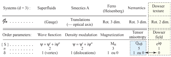
Figure 4.1. Classification of topological defects in systems with an order parameter, proposed by de Gennes (1972). d is the dimension of space in which the system exists, n is the number of components of the order parameter and δ is the dimension of the defects, which is 0 for points (monopoles) and 1 for lines (dislocations, disclinations or vortices). Adapted from de Gennes (1972)
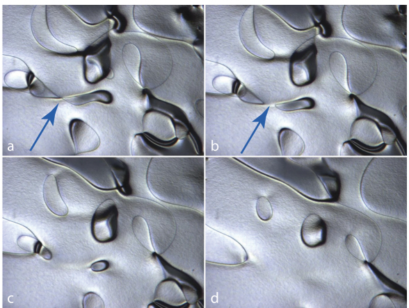
Figure 4.2. Spontaneous shrinking and collapse of disclination loops in a nematic droplet
- 1) they can be threaded on solid inclusions or fibers (Čopar et al. 2016), where the repulsive interaction with surfaces opposes their collapse (see Figure 4.3(a));
- 2) they can be stabilized or set into motion by the action of magnetic fields in twisted nematic cells (see Figure 4.3(b));
- 3) they can be stabilized by the action of special anchoring patterns (see Figure 4.3(c)).
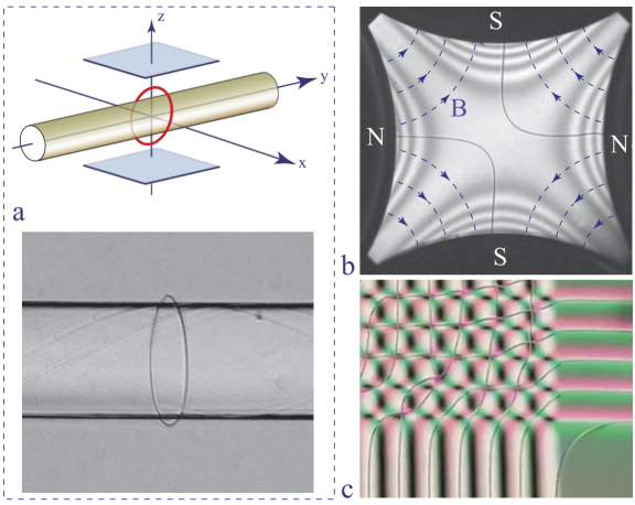
Figure 4.3. Stable systems of disclinations. (a) Disclination loop threaded on a polymeric fiber (Čopar et al. 2016; Cabeça et al. 2019). (b) Disclinations in a twisted nematic cell stabilized by a quadrupolar magnetic field (Srinivasan 2020). (c) Web of disclinations generated by patterned anchoring conditions (Wang et al. 2017) (courtesy of Wang and Yokoyama)
4.1.1.2. Monopoles are scarce
In contradistinction to disclinations, monopoles are scarce (Hindmarsh 1995). They are absent in the images in Figure 4.2, which means that they were not generated like the disclinations by stirring. The occurrence of monopoles requires special geometries of the limit surfaces and of the anchoring conditions on them:
- 1) monopoles occur as companions of inclusions with homeotropic anchoring conditions (Poulin et al. 1997; Musěvič et al. 2006) (see Figure 4.4(a));
- 2) they can be generated by the isotropic–nematic quench in capillaries with homeotropic anchoring conditions (Meyer 1972), (Williams et al. 1972), (Cladis and Brand 2003) (see Figures 4.4(b) and 4.5(f));
- 3) they can be easily generated, set into motion and brought into collisions in the so-called dowser texture, as we will point out below (see also Pieranski et al. (2016a,b) and Pieranski and Godinho (2020)) (see Figure 4.4(c)).
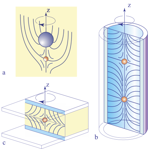
Figure 4.4. Occurrence of nematic monopoles: (a) as companions of inclusions with homeotropic anchoring, (b) induced by homeotropic anchoring in capillaries, (c) as defects of the dowser texture
4.1.1.3. Disclinations and monopoles as topological defects
The contrast between the ubiquity of disclinations and the scarcity of monopoles has topological reasons (Kleman and Lavrentovich 2006). Figure 4.5 shows that the director field on a circuit surrounding a disclination (Figure 4.5(a)) is mapped on just one meridian on the eastern hemisphere, which represents the space (real projective plane) of the nematic order parameter (Figure 4.5(b)). Therefore, to generate a disclination during the isotropic–nematic quench, it is enough to have three adjacent nematic-in-isotropic droplets with adequate orientations (Figure 4.5(c)). After the coalescence of droplets, the disclination must appear there.
A similar bulk mechanism is very unlikely in the case of the monopole because the director field on a surface surrounding it (Figure 4.5(d)) is much more complex: it is mapped twice on the space of the nematic order parameter, once on the whole northern hemisphere and the second time on the whole southern hemisphere (Figure 4.5(e)). However, when the isotropic–nematic quench is realized in a capillary with homeotropic anchoring conditions, monopoles must appear between the adjacent domains with escaped director fields (Figure 4.5(f)).
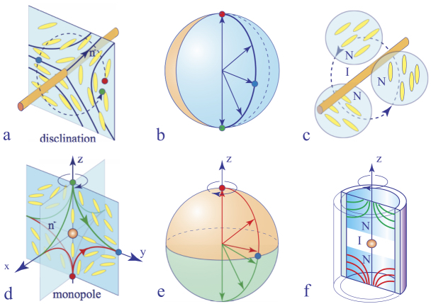
Figure 4.5. Topology of disclinations and monopoles
4.1.2. Road to the dowser texture
4.1.2.1. Difficulties with nematic monopoles in the dowser texture
In principle, for the same reason as adequate boundary conditions, a monopole can exist in a nematic droplet maintained by a capillarity between two surfaces with homeotropic boundary conditions, as shown in Figure 4.6. However, in practice, a different configuration, shown in the Figures 4.6(a) and (c) arises after the introduction of the drop in the gap between the glass slide and the lens. Here, the homeotropic texture (represented by the black disc in Figure 4.6(c)) coexists with a distorted texture, also satisfying the homeotropic boundary conditions (colored and black interference fringes in polarized light), in which the director rotates by π between the limit surfaces. The homeotropic and distorted textures are separated by a disclination loop.
The name of the distorted texture varied in past. It was called the “splay-bend state” by Cladis et al. (1987), the “H state” by Boyd et al. (1980), the “inversion wall” by Gilli et al. (1997), the “quasi-planar state” by Fazzio et al. (2001) or “flow-aligned” by Giomi et al. (2017). In Pieranski et al. (2016a), we proposed to call it “the dowser texture” because the director field lines in it have shapes similar to that of a Y-shaped wooden dowser’s tool. This name will be used throughout this chapter.
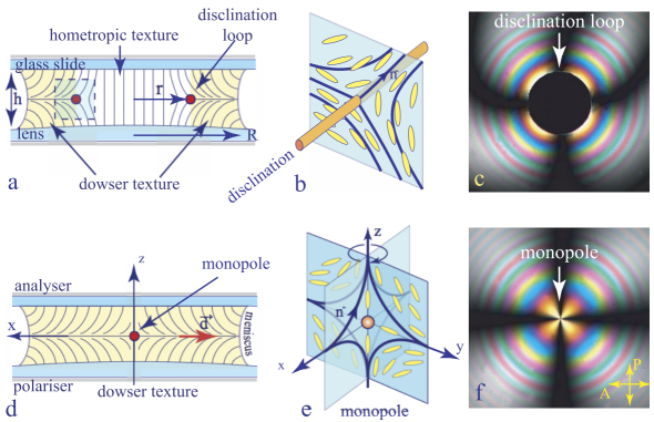
Figure 4.6. The dowser texture. (a) Coexistence of the dowser and homeotropic textures. (b) Disclination at the border between the dowser and homeotropic textures. (c and f) Views in a polarizing microscope. (d and e) Nematic monopole in the dowser texture
As it is distorted, the dowser texture has the elastic energy per unit area of the order of
so that it is energetically less favorable than the homogeneous homeotropic one.
Therefore, usually its area shrinks for the benefit of the homeotropic texture (circle of radius r). The expansion of the homeotropic texture is stopped when the disclination reaches the border of the droplet, where it is repelled by an elastic interaction with the meniscus with homeotropic anchoring. Let us emphasize that after its expansion, the disclination does not disappear but remains in the vicinity of the meniscus, where its radius r is slightly smaller than the droplet’s radius R. The annular domain between r and R is filled with the residual dowser texture.
In view of such observations made commonly during the preparation of homeotropic cells, the dowser texture was believed to be unstable for decades and little attention was paid to it.
4.1.2.2. Generic experiments
This belief was first broken by Gilli et al. (1997) and more recently by Pieranski et al. (2016a) during experiments with disclinations threaded on polymeric fibers, where it was found that the residual dowser texture can expand at the expense of the homeotropic texture when the radius/thickness ratio r/h is small enough.
The generic experiment started with the homeotropic texture filling the droplet, except for an annular domain of the residual dowser texture in the vicinity of the meniscus (see Figure 4.7(a)). An unexpected phenomenon occurred when the thickness h of the gap was increased to about 1.5 mm. The series of four pictures in Figure 4.7(b) shows that the peripheral disclination shrunk and coalesced with the captive disclination. As a result, the dowser texture filled the whole volume of the droplet.

Figure 4.7. Generic experiment paving the way to the dowser texture. (a) Perspective view of the setup for studies of captive disclinations. (b) Surprising collapse of the peripheral disclination
This first observation of the expansion of the dowser texture was confirmed in a second experiment performed in the absence of the polymeric fiber. It is illustrated here, by a series of three pictures in Figure 4.8. No longer being hindered by the polymeric fiber, the peripheral disclination collapses into a point – a nematic monopole.
4.1.2.3. Relative stability of the homeotropic and dowser textures
To explain how the expansion of the dowser texture is possible, we must take into account the elastic energy 2πrT of the disclination (of radius r and tension T) located, for topological reasons, at the frontier between the dowser and homeotropic textures (see Figure 4.6(a)). It has to be added to the elastic energy of the dowser texture in its volume π(R2 − r2)h. The total energy
has a maximum at

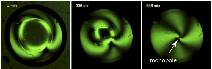
Figure 4.8. Collapse of the peripheral disclination into a monopole
Usually, during the preparation of homeotropic samples, the typical thickness h = 100 mμ is small and the critical radius rcrit ≈ 2h is also small. Therefore, the radius of the homeotropic domain coexisting with the dowser texture is larger than the critical radius r > rcrit, so that the homeotropic domain expands and fills the droplet. As this implicit condition was always satisfied during the preparation of homeotropic samples, the belief in the instability of the dowser texture was founded on it.
In the generic experiment with the captive disclination, the initial thickness was about 300 μm. For the volume πR2h ≈ 10 mm3, the corresponding radius of the drop was R = 2.5 mm. The corresponding point H in the graph of Figure 4.9(e) is located in the area of stability of the homeotropic texture. Subsequently, with V = const and increasing thickness h, the radius R of the droplet decreased along the hyperbolic trajectory (the dotted blue line from H to D). With the disclination remaining in the vicinity of the meniscus, the ratio r/h ≈ R/h decreased and crossed the critical value ≈ 2 (represented by the red line in Figure 4.9(e)), and the dowser texture started to expand.

Figure 4.9. Three-stage road to the dowser texture. (a–d) Schematic representation of the method. (e) Corresponding trajectory on the R-vs-H diagram
4.1.2.4. Persistence of the dowser texture
This first surprising observation was followed by a second: upon the reduction of the sample thickness along the red dotted trajectory from D to D’ in Figure 4.9(e), the critical line R/h ≈ 2 was crossed again in the opposite direction but, surprisingly, the dowser texture persisted until the gap thickness h was reduced to below ≈ 1 μm. In such a case, the monopole (Figure 4.5(c)) “blows up” into a disclination loop (Figure 4.5(f)) with a growing radius and the homeotropic texture is recovered.
This observation of the surprising persistence of the dowser texture opened the door to experiments with it. We will point out below that the dowser texture is worthy of its name, not only because of the shape of the director field in it, but also because it can be used as a probe of fields, such as the velocity v of Poiseuille flows, electric fields E and thickness gradients g =∇h.
4.1.3. The dowser texture
4.1.3.1. Order parameters of the dowser texture, the dowser field
In the table of topological defects proposed by de Gennes (Figure 4.1), nematic monopoles appear in the column “Nematics” as point defects of dimension δ = 0 of the tensorial order parameter Qαβ, with generally n = 5 components in the three-dimensional nematic phase (for uniaxial nematics,n=3).
The director field n(x,y,z) of the dowser texture in a thin nematic layer of thickness h can be expressed as
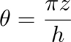
with the polar angle θ varying from −π/4 on the lower surface to π/4 on the upper surface.
In the experiments discussed here, with the exception of the flow-induced homeotropic-dowser transition, the polar angle does not depend on x and y and conserves the same variation with z (in approximation of an isotropic elasticity)


Figure 4.10. Defects in systems with complex order parameters: (a) vortices in a superconductor, (b) dislocation in a Blue Phase crystal, (c) disclination in a SmC film, (d) umbilic in a nematic layer and (e) monopole in the dowser texture (adapted from Pieranski (2019))
On the other hand, the azimuthal angle φ of the director only depends on x and y coordinates (see Figures 4.10(e) and 4.11(c)), so that we can write
with ez = [0, 0, 1] and
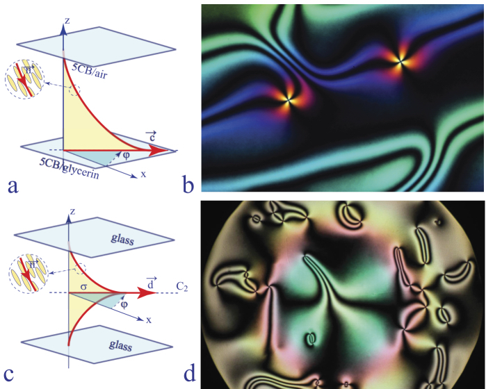
Figure 4.11. Nematic layers with degenerated anchoring conditions. (a) Film of 5CB floating on the surface of glycerin, investigated by Lavrentovich and Rozhkov (1988). The anchoring at the glycerin/5CB and air/CB interfaces is, respectively, planar and homeotropic. (b) Typical “schlieren” picture (courtesy of Lavrentovich). (c) The dowser texture between glass surfaces with homeotropic anchoring. (d) Typical “schlieren” texture
In this approximation, we can consider the dowser texture as a two-dimensional (2D) system with the unitary 2D vector order parameter d or, equivalently, with an unidimensional complex order parameter eiφ. Taking this into account, we added the last column to the de Gennes’ table in Figure 4.1. Nematic monopoles can now also be seen as topological defects of the complex order parameter eiφ and are therefore analogous to vortices or dislocations.
Let us note that the unitary 2D vector field d = (cos φ, sin φ) – that we call the dowser field – is similar to the c field in Smectics C films or in a homeotropic nematic layer above the Fréedericksz transition, as well as in a nematic layer floating on glycerin (Lavrentovich and Rozhkov 1988). These analogies are summarized in Figures 4.10 and 4.11.

Figure 4.12. Monopole–antimonopole pair generated in a dowsons collider. (a) View in a polarizing microscope. (b) Phase φ(x,y) and dowser d(x,y) fields around the pair. (c and d) Detailed phase and dowser fields of the monopole (d) and antimonopole (c)
4.1.3.2. Dowser texture as a natural universe of monopoles
Since the discovery of its persistence, the dowser texture was extensively studied with the particular aim of generating and manipulating monopoles. A series of setups tailored for this purpose was developed (see section 4.2.1). They were used, among others, to generate monopoles, such as the pair shown in Figure 4.12(a). From the interference fringes (isogyres), we inferred the phase field φ(x, y) and the dowser field d(x, y) surrounding this pair (see Figure 4.12(b)). The phase field is coded using the colors defined in Figures 4.12(c) and (d), where the dowser field is represented by arrows in the same figures. Clearly, on the circuits surrounding these two monopoles, the defect of the phase is Δφ = +2π and Δφ = −2π as indicated. By convention, the monopole with Δφ = −2π will be called an antimonopole.
Our setups were also used to set monopoles and antimonopoles in motion on trajectories leading to collisions, which can result in the annihilation of monopole–antimonopole pairs (see Figure 4.13). By analogy with the hadron colliders, these setups are called dowsons colliders because monopoles and antimonopoles occurring in the dowser texture are dubbed, in short, dowsons d+ and d-.
A typical result obtained with a dowsons collider is shown in Figure 4.13. On this image obtained by the superposition of 32 pictures taken at intervals of 10 s, the trajectories of dowsons d+ and d- appear as dotted lines. Yellow and blue arrows indicate the initial position dowsons. The collisions of pairs (d+,d-) are indicated by circles, which are, respectively, drawn with a solid line when annihilations occur, or with a dotted line when the colliding dowsons are passing by.

Figure 4.13. Collisions of monopole/antimonopole pairs in a dowsons collider. Superposition of images taken at intervals of 10 s. Yellow and blue arrows indicate the initial positions of monopoles and antimonopoles circulating in opposite directions. Collisions are indicated with circles drawn with a solid line when annihilation occurs or with a dotted line when monopoles are passing by
Today, because of these studies with dowsons colliders, monopoles can no longer be considered as scarce. On the contrary, they appear as topological defects that are very easy to generate and manipulate, as we will show in sections 4.8–4.10. In view of these achievements, the dowser texture appears today as a natural universe of nematic monopoles.
4.1.3.3. Tropisms of the dowser texture
Experiments with dowsons colliders also allowed the discovery of remarkable properties of the dowser texture itself that arise from its symmetry C2v, which only contains three elements: the twofold axis C2 and two mirror planes passing through it: σ (see Figure 4.14(a)) and σ’ passing, respectively, through z and x axes. The group C2v is a subgroup of D∞h – the symmetry group of the cell filled with the isotropic phase or with the homeotropic texture (Figure 4.14(a)). The order parameters d or eiφ resulting from the D∞h ![]() C2v symmetry breaking are thus degenerated with respect to rotation around the z axis. For this reason, the dowser texture is expected to be very sensitive, in first order, to fields f. As we will see in the following sections, fields f, such as thickness gradient g =∇h, Poiseuille flow v or the electric field E exert on the dowser field d torques given by
C2v symmetry breaking are thus degenerated with respect to rotation around the z axis. For this reason, the dowser texture is expected to be very sensitive, in first order, to fields f. As we will see in the following sections, fields f, such as thickness gradient g =∇h, Poiseuille flow v or the electric field E exert on the dowser field d torques given by
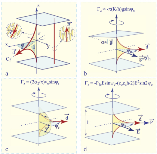
Figure 4.14. Tropisms of the dowser texture. (a) Symmetry of the dowser texture and its order parameters φ and d. (b) Cuneitropism: alignment by the thickness gradient g =∇h. (c) Rheotropism: alignment by the Poiseuille flow v. (d) Electrotropism: alignment by the electric field E
Upon the action of these torques, the dowser field d tends to be aligned in the direction parallel (or antiparallel) to f. In other words, we can concisely say that the dowser texture possesses the following tropisms:
- – cuneitropism: alignment by thickness gradient g (see section 4.5);
- – rheotropism: alignment by Poiseuille flows v (see section 4.4);
- – electrotropism: alignment by electric fields E (see section 4.6).
4.2. Generation of the dowser texture
4.2.1. Setups called “Dowsons Colliders”
Several setups were developed as we progressed in studies of the dowser texture. They were tailored with the aim of accomplishing several tasks, starting with the necessary preparation of the dowser texture.
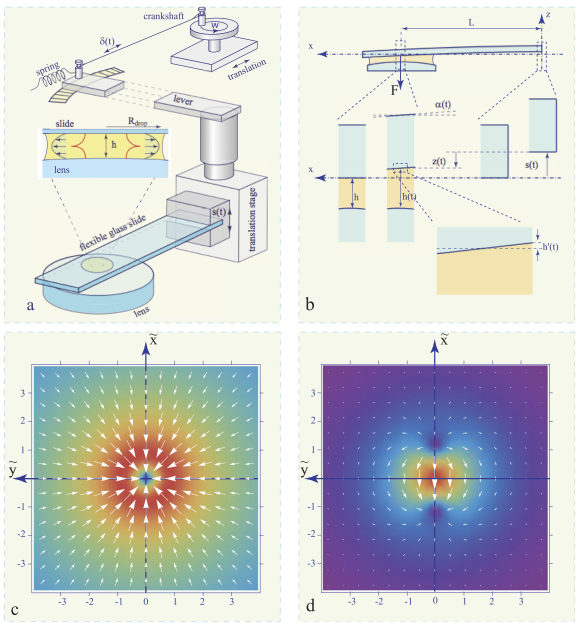
Figure 4.15. Generic setup called Double Dowsons Collider 1 (DDC1). (a) General view. (b) Up and down translation s(t) and flexion α(t) of the glass slide. (c) Radial flow driven by an upward translation of the slide. (d) Dipolar flow driven by the flexion α(t) of the slide. Remark: Radial and polar flows are shifted in phase by π/2
All of these setups have two elements in common (see Figure 4.15): a microscope glass slide (75×19×0.9 mm) and a lens (50 mm in diameter with the radius of curvature Rl=140 mm), both mounted on a vertical bench. The lens is fixed, while the glass slide is movable by means of precise translation stages in x, y and z directions.
The motion in z direction allows the control of the thickness h of the slide/lens gap that, by capillarity, keeps the nematic drop in its center of minimum thickness h.
4.2.2. “Classical” generation of the dowser texture
The scheme of the very first setup in Figure 4.15 shows that precision of the vertical motion s(t) is improved by means of a lever (24 cm in length) attached to the micrometric screw of the translation stage. Using this system, we can thus control the thickness h and generate the dowser texture using a three-stage process, discussed in section 4.1.2.1, which consists of following the path H→D→D’ indicated by the dotted lines in the graph in Figure 4.9(e).
The initial thickness (minimal thickness at the center of the gap) and radius R of the nematic droplet at the point H do not matter, but are typically of the order of h ≈ 300 mμ and R ≈ 3 mm. Subsequently, the point D is reached by increasing the thickness to h≈1.5 mm and the collapse of the peripheral disclination (illustrated by schemes b to c in Figure 4.9, h = 1.4 mm) is initiated, as already discussed in section 4.1.2.1 (see Figure 4.8).
Let us stress that the collapse of a large homeotropic domain encircled by the disclination loop is a very slow process that can last several hours. In the example of Figure 4.8, 11 hours were necessary for the peripheral disclination to collapse into the residual monopole situated in the center of the droplet.
After the collapse of the peripheral disclination, the thickness is slowly reduced to about 10 mμ, and the final point D’ of the H→D→D’ path in Figure 4.9(e) is reached.
4.2.3. Accelerated generation of the dowser texture using the DDC2 setup
The generation of the dowser texture can be shortened from hours to about one minute using another version of the Double Dowsons Collider, called DDC2, which will be described in section 4.4.3.1. The operational principle of this second method involves four stages:
- 1) Shreding: A vigorous streaming flow inside the droplet, driven by flexural vibrations of the flexible glass plate, stretches and shreds the unique homeotropic-in-dowser domain (r≈1.5 mm) into a multitude of small domains (see Figure 4.16), with radii ri ≈20 μm. The streaming flow also shifts the nematic droplet as a whole on the distance Δy.
- 2) Flow-induced homeotropic
 dowser transition: After cessation of the streaming flow, the drop returns, by capillarity, to the initial position. The Poiseuille flow accompanying this translation reduces the radii of the small homeotropic-in-dowser domains; it is an evidence of a flow-induced homeotropic ⇒ dowser transition.
 - 3) Increase of the thickness: A subsequent increase in the gap thickness reduces radii ri below the critical value rc and the collapse of the homeotropic-in-dowser domains occurs rapidly.
- 4) Reduction of the thickness: Once all homeotropic-in-dowser domains have disappeared, the thickness of the gap can be reduced accordingly.
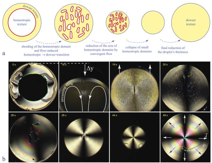
Figure 4.16. Shortening of preparation of the dowser texture by a transitory application of a turbulent mixing
The second stage of this process is related to the recent works by Emeršič et al. (2019) and Liu et al. (2019), who used microfluidic methods to study the relative stability of the homeotropic and dowser textures in the presence of a Poiseuille flow. Inspired by these works, we used our setup to explore the flow-induced homeotropic ⇒ dowser transition in more detail.
4.3. Flow-assisted homeotropic ⇒ dowser transition
4.3.1. Experiment using the DDC2 setup
Our experiments started by the generation of a unique homeotropic-in-dowser domain by means of a reduction of the gap slide/lens thickness to zero (see the series of three pictures in Figure 4.17). After its nucleation, the homeotropic-in-dowser domain is expanding. Once its radius r is large enough, the minimal thickness is increased to h = 60 μm. By means of this method, it is possible to generate H-in-D domains with different radii r.

Figure 4.17. Generation of a unique homeotropic-in-dowser domain by the reduction of the slide/lens gap to zero. (a) The radial dowser texture with the minimal thickness h close to zero, favoring nucleation of the homeotropic domain. (b and c) Expansion of the homeotropic domain
Subsequently, the H-in-D domains were submitted to slow streaming flows with velocities set to such values vc that the sizes rc of domains were conserved. One of these experiments is illustrated by the spatiotemporal cross-section in Figure 4.18(a). Initially, the size rc of the domain is relatively small and the slope vc of the domain’s trajectory in the (t,x) plane is also relatively small. Subsequently, the streaming flow is stopped and the size rc of the domain grows a little until the streaming flow is applied once again and adjusted to a new stationary value vc, which is larger than the first one. In the last growth-adjustment sequence visible at the end of the spatiotemporal cross-section in the Figure 4.18(a), vc is even larger.
Results of several such experiments are represented by red crosses in the upper part of the plot 1/rc versus vc, as shown in Figure 4.18(c). They fit well to the linear law

with rco = 69 μm and vco = 3.9 μms−1.

Figure 4.18. Stability of homeotropic-in-dowser domains in Poiseuille flows. (a) Spatiotemporal cross-section showing the motion of a homeotropic-in-dowser domain. (b) Homeotropic and dowser textures submitted to a Poiseuille flow. (c) Stability diagram. Red crosses – experimental points extracted from the spatiotemporal cross-sections, such as the one in (a). Blue crosses – experimental data from figure 2G in Emeršič et al. (2019). Solid red line – fit to the equation [4.9]. (5CB, h = 60μm)
![]() et al. (2019), in their experiments with microfluidic channels, studied the flow-induced homeotropic-dowser transition in the complementary geometry of dowser-in-homeotropic domains. Their results, obtained with a channel of thickness h=12 μm, are represented by blue crosses in the lower part of the plot in Figure 4.18c. They are fitted to the same linear law with rco = 10 μm and vco = 56 μ ms−1. Let us note that the red line of the linear fit extends to the left part of the plot with negative values of velocity. So far, experimental points are missing, but at the end of the theoretical section below we will suggest how they can be obtained.
et al. (2019), in their experiments with microfluidic channels, studied the flow-induced homeotropic-dowser transition in the complementary geometry of dowser-in-homeotropic domains. Their results, obtained with a channel of thickness h=12 μm, are represented by blue crosses in the lower part of the plot in Figure 4.18c. They are fitted to the same linear law with rco = 10 μm and vco = 56 μ ms−1. Let us note that the red line of the linear fit extends to the left part of the plot with negative values of velocity. So far, experimental points are missing, but at the end of the theoretical section below we will suggest how they can be obtained.
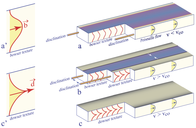
Figure 4.19. Flow-assisted bowser-dowser transformation in a capillary. (a,a’) For v < vco, the bowser texture fills the capillary except for thin dowser boundary layers at lateral walls. (b) For v > vco, the flow-assisted bowser-dowser transformation occurs. The width of the dowser boundary layers grows. (c,c’) The capillary filled with the dowser texture
4.3.2. Flow-assisted bowser-dowser transformation in capillaries
Liu et al. (2019) investigated the flow-assisted homeotropic-dowser transformation occurring in long straight capillaries with rectangular cross-sections, in detail. In the absence of flows, the ground state of the director field corresponds to the homeotropic texture, filling the capillary, except for the thin boundary layers of the dowser texture at lateral capillary’s walls. As the disclinations separating the dowser boundary layer from the bulk homeotropic texture are straight (see Figure 4.82(a)), this experiment corresponds to the case rc → ∞, i.e. 1/rc = 0, in Figure 4.18(c).
When the flow velocity is smaller than the critical value vco, the homeotropic texture is deformed into the bowser texture, but disclinations remain in the vicinity of the lateral walls (see Figure 4.19(a)). For v > vco, an instability occurs: the dowser boundary layers become progressively broader (see (Figure 4.19(b)) until they coalesce and the whole capillary is filled with the dowser texture (see Figure 4.19(c)).
Using, for example, a channel of thickness h = 50 μm, Liu et al. obtained vco = 9 μms−1.
4.3.3. Flow-assisted homeotropic-dowser transition in the CDC2 setup
Anticipating the description of the so-called Circular Dowsons Collider 2 (see Figure 4.28) that will be given in section 4.4.3.3, let us report on the flow-assisted homeotropic-dowser transition realized by means of this setup. CDC2 was tailored for the winding of the dowser texture and for experiments on the generation, motions and collisions of dowsons.
For large amplitudes of the conical motion of the glass slide, CDC2 generates a stationary circular flow with the orthoradial velocity vmax (see Figure 4.20(b)), growing with the distance r from the center. The experiment illustrated in Figure 4.20 starts with a relatively large circular homeotropic-in-dowser domain located in the center of the nematic droplet (see Figure 4.20(a)). The circular streaming flow of amplitude vmax(r) generated in the droplet is thus parallel to the homeotropic/dowser interface of radius r (see Figure 4.20(b)). The subsequent evolution of the radius r(t) depends on the initial velocity vmax(t = 0) of the flow. Let us suppose that at t = 0 and r = r(0) (point t = 0 in Figure 4.20(h)), the velocity vmax = v(r(0)) is larger than the critical velocity vc(r) (red line in Figure 4.20(h)) defined by equation [4.9], so that the homeotropic-in-dowser domain starts to shrink. Let us suppose next, in the first approximation, that the velocity vmax(r) is proportional to the radius: vmax = ωr or alternatively, that
In Figure 4.20(h), this variation is represented by the hyperbola drawn with a dotted red line. The stationary state is reached at the intersection labeled SS of the red and dotted lines, in which the radius rss of the homeotropic (bowser) domain is reduced with respect to r(0).
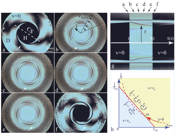
Figure 4.20. Flow-assisted hemeotropic-dowser transition in the circular geometry of the CDC2 setup (see section 4.4.3.3). (a) Circular homeotropic-in-dowser domain expanding in the absence of flow. (b–e) Shrinking of the homeotropic-in-dowser domain induced by the circular streaming flow revealed by motion of a dust particle indicated by arrows. (f) Homeotropic-in-dowser domain expanding after cessation of the streaming flow. (g) Spatiotemporal cross-section extracted from a video along the line CS, defined in (a). (h) Theoretical explanation of the experiment
In the experiment depicted in Figures 4.20(a–f), the radius r ≈ 1.5 μm is 22 times larger than the critical radius rco = 69 μm. Therefore, the critical velocity vss = 22 μm/s measured in the stationary state SS is close to critical velocity vco (in the limit r → ∞).
4.3.4. Theory of the flow-assisted homeotropic-dowser transition
The explanation of the linear dependence between the critical curvature 1/rc of the homeotropic/dowser interface and the flow velocity vc was first proposed by Emeršič et al. (2019). More recently, Tang and Selinger (2020) developed this theory and presented it in detail. Here, we will analyze the flow-assisted homeotropic-dowser transition in slightly different terms.
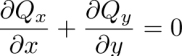
Let us start with the expression of the viscous torque per unit volume exerted by a shear flow on the director (see, e.g. de Gennes and Prost (1993) or section III.4 in Oswald and Pieranski (2005)).
We will first suppose that the stationary deformations of the homeotropic and dowser textures, due to this torque, are so small that they can be neglected. This is true when the Poiseuille flow is slow enough. During the expansion of the dowser texture across the strip of width dx (see Figure 4.18(b)), the polar angle at the point P (in the upper half of the nematic layer) decreases from π/2 to πz/h and the torque Γz does the work (per unit volume)

Knowing that the shear rate in the Poiseuille flow is dv/dz = −8vmaxz/h2, we obtain, by integration on z, the work per unit area
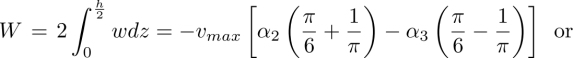
The factor 2 in equation [4.13] takes the same work done by the viscous torque in the lower half of the nematic layer into account. This work corresponds to an effective potential Ueff =-W (Tang and Selinger 2020), which has to be added to the total elastic energy given in equation [4.2]:

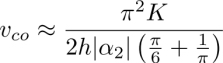
The maximum of F’ is located at

This expression justifies the linear law in equation [4.9], used above for the fit of experimental data.
4.3.5. Summary and discussion of experimental results
All experiments on the flow-assisted homeotropic-dowser transition were made with 5CB. As in this material |α3| << |α2| (Ternet et al. 1999; Blinov and Chigrinov 1996), the expression of the critical velocity in equation [4.16] can be simplified to
As the flow-induced homeotropic-dowser transition in the straight capillary (section 4.3.2) is a kind of hydrodynamic instability (such as those discussed in chapter III.4 in Oswald and Pieranski (2005)), it is convenient to define an Ericksen number
and rewrite equation [4.17] of the critical velocity as
Using K ≈ 5.5 · 10−12N, |α2| ≈ 0.83Pa · s (Oswald et al. 2013; Blinov and Chigrinov 1996) and the values of the thickness h and the critical velocity vco measured experimentally, we obtain:
- – Erc=10, with h=12 μm and vco=56 μm/s in Emeršič et al. (2019);
- – Erc=6.7, with h=50 μm and vco=9 μm/s in Liu et al. (2019);
- – Erc=4.7, with h=60 μm and vco=3.2 μm/s in section 4.3.1;
- – Erc=19.8, with h=30 μm and vco ≈ 22 μm/s in section 4.3.3.
4.4. Rheotropism
4.4.1. The first evidence of the rheotropism
4.4.1.1. Experiment
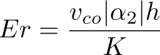
During the last stage of the preparation of the dowser texture, the thickness h is reduced from about 300 to 10 μm and the dowser texture is submitted to a Poiseuille flow directed outward. At first glance, it is obvious from the interference pattern in Figure 4.21(b) that this diverging flow (see Figure 4.21(a)) very efficiently orients the dowser field d in the outward radial direction. This is the first manifestation of the rheotropism of the dowser texture, which is analogous to the behavior of a weather vane indicating the wind’s direction (see Figure 4.22(b)).
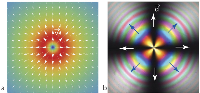
Figure 4.21. Alignment of the dowser field by a radial Poiseuille flow directed outward. (a) Flow pattern. (b) Dowser field inferred from the interference pattern
4.4.1.2. Theory of the rheotropism
Theoretically, rheotropism is expected as a consequence of hydrodynamic torques exerted on molecules by Poiseuille flows (see section 4.16.2). More precisely, the rotation of the dowser texture around the vertical z axis is due to the z component Γz of the hydrodynamic torque exerted by a Poiseuille flow v(z) on the director n(z). To calculate this torque, we will use a local reference frame (ξ, η, z) with the ξ axis parallel to d (see Figure 4.22). If ψ is the angle between the ξ axis and the plane of the Poiseuille flow, then the flow velocity v can be expressed as v = v(cosψ, sinψ, 0).
The hydrodynamic torque produced by the vξ component of the flow only has the Γη component, which only acts on the polar angle θ of the director (see Figure 4.22(a))). We will suppose in the following that its effects are negligible.
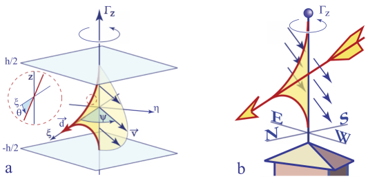
Figure 4.22. The origin of the rheotropism. (a) Hydrodynamic torque Γz exerted by the Poiseuille flow on the dowser texture. (b) Analogy with a weather vane
The Γz component of the hydrodynamic torque is produced exclusively by the vη component of the Poiseuille flow and, when calculated per unit area in the xy plane, it is written as:

where α2 is the Leslie viscosity coefficient (α2 < 0 in 5CB).
With
and

we get:
As this torque vanishes for ψ = 0, i.e. when the dowser texture is aligned with the velocity v, the weather vane-like behavior is justified. The torque Γz also vanishes for ψ = π, i.e. in the antiparallel position, but this orientation of the dowser field d antiparallel to the flow v is unstable.
In the laboratory reference frame, this rheotropic torque can be alternatively expressed as:
withIn the divergent flow, the amplitude of the rheotropic torque depends on the distance r from the gap center, because the velocity of the Poiseuille flow vmax(r) is a function of r. To calculate this dependence, one can start from the expression of the total flux Φ through a cylindrical cross-section of radius r:
Knowing that the thickness h(r) of the gap between the slide and the spherical surface of the lens, with radius of curvature Rl is given by
we obtain
The color code in Figure 4.21(a) shows that the velocity of the Poiseuille flow in the gap has a maximum at ![]() Typically, with hmin=10 μm and Rl=140 mm, we obtain rmax=1.7 mm.
Typically, with hmin=10 μm and Rl=140 mm, we obtain rmax=1.7 mm.
4.4.2. Synchronous winding of the dowser field
4.4.2.1. Experiment
Experiments with the DDC1 setup shown in Figure 4.15 unveiled another, more sophisticated consequence of the rheotropism: the winding of the dowser texture.
This new phenomenon is illustrated by the series of nine pictures in Figure 4.23, taken during the first period of a harmonic up and down motion of the glass slide: s(t) = sosin(ωt). (To be more precise, we should say “of the support of the glass slide”. The importance of this detail will be discussed in section 4.4.2.2).

Figure 4.23. Evolution of the dowser texture during one period of the up and down motion of the glass slide
The deformation of the initial cross-shaped pattern of isogyres (black fringes) shows that the dowser field, initially oriented in the outward radial direction, is perturbed by the flow. If we follow the orientation of the dowser field d inside the square dotted area, it is obvious that, at the end of this first period of excitation, a rotation by 2π occurred here in the anticlockwise direction. On the other hand, inside the dotted circular area, the dowser field returns to its initial radial orientation after a clockwise-anticlockwise oscillation. As a result, a 2π-wall, visible in Figure 4.23(i), is created during this first period of excitation. In the right half of the droplet, the dowser field rotates by -2π in the clockwise direction so that another symmetrically disposed 2π-wall is created here.
The continuation of this experiment is illustrated in Figure 4.24. Here, pictures a-k have been extracted from a video at ends of 10 consecutive periods T of excitation, while the image in the center represents the spatiotemporal cross-section composed of lines extracted from all frames of the whole video.

Figure 4.24. Winding of the dowser texture by harmonic motion of the glass slide in the DDC in Figure 4.15
The most important result inferred from this experiment is that in the left and right halves of the droplet the dowser field d is rotating, respectively, in anticlockwise and clockwise directions. As this process is similar to the winding of an elastic strip (shown in Figure 4.25(b)), we call it the “winding of the dowser field”. Moreover, as the maximal angular velocities of the rotating dowser field are < ωw >= ±2π/T , this winding process is synchronous with the excitation of frequency ωexc = 2π/T. The analogy with the winding of an elastic strip is not complete because in the more detailed view of the dotted rectangle (defined in Figure 4.25(a)) shown in Figure 4.25(c) the black isogyres have variable width and are not equidistant. The corresponding variation of the azimuthal angle φ with x can be expressed as:

Figure 4.25. Mechanical analogies of the wound up dowser texture. (a) Detailed view of the picture l in Figure 4.24. (b) Winding of an elastic strip. (c) detailed view of the dowser field. (d) Winding of a chain of pendula attached to an elastic string
This expression describes the state of equilibrium of a continuous wound up chain of pendula attached to an elastic wire and submitted to the gravity g. It is a solution of the equation
which describes the balance of the elastic and the gravitational torque (ρ is the mass per unit length of the chain, l is the length of pendula and g is the gravitational acceleration).
In section 4.5, we will see that an analogous equation applies to the case of a dowser field wound up in x direction, for which the first term also expresses the elastic torque, while the second term is due to the cuneitropism: the torque (πK/h)sin φ tends to orient the dowser field in the direction of the thickness gradient. In the gap between the spherical lens and the flat glass slide, the thickness gradien ![]() radial and directed outward. In the small rectangular dotted area, it is antiparallel to the x axis.
radial and directed outward. In the small rectangular dotted area, it is antiparallel to the x axis.
4.4.2.2. Interpretation in terms of the rheotropism
The winding of the dowser field cannot be due to the Poiseuille flows driven exclusively by the harmonic up and down translation s(t) = so sin(ωt) of the glass slide. Indeed, such flows are radial and have symmetry of revolution around the z axis, while the pattern of isogyres of the wound up dowser field is only symmetrical with respect to the (x,z) mirror plane. Starting from this striking disagreement, we also have to take the dipolar flows driven by the flexion of the elastic glass slide into account.
Figures 4.15(a) and (b) show that the glass slide is clamped and attached to the translation stage at only one of its extremities. The flexion of the glass slide is due to the viscous stress σzz, in the squeezed or stretched droplet, which is proportional to dh/dt. The tilt angle α of the glass plate in the center of the droplet is therefore proportional to dh/dt.
The tilt of the glass plate taken alone generates a dipolar flow represented in Figure 4.15(c). Here, it was calculated approximatively as a superposition of two radial flows: the first one diverging from a point source and the second one converging to a point well. The source and the well are located, respectively, at (0,yo) and (0, −yo). These radial flows are proportional to dα/dt ∼ d2h/dt2.
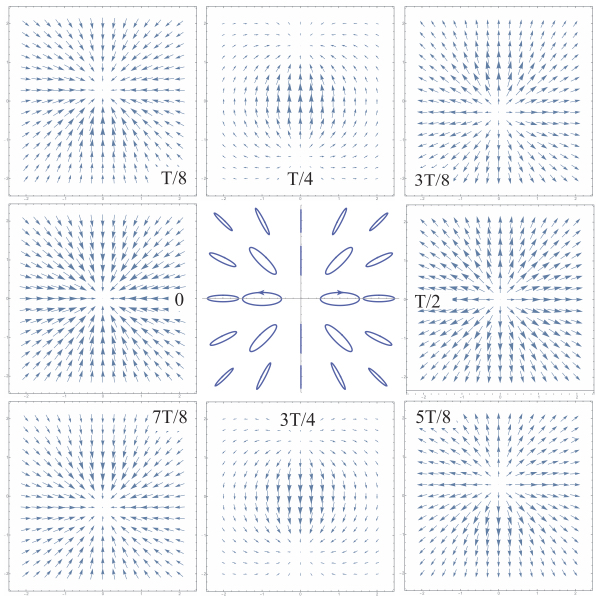
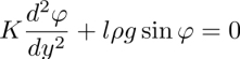
Figure 4.26. Flows inside a nematic droplet driven by a harmonic up and down motion s(t) in the Double Dowsons Collider 1 (see Figure 4.15). Pictures labeled 0, T/8,...,7T/8 show the flow patterns at intervals of T/8. The picture in the center shows trajectories of molecules
Being proportional, as stated above, to respectively dh/dt and d2h/dt2, the radial and dipolar flows are thus shifted in phase by π/2.
The sum of these radial and dipolar flows is illustrated by the series of eight pictures in Figure 4.26. The most significative is the picture in the center that shows local trajectories of molecules: they are elliptical anticlockwise and clockwise in the left and right halves of the drop, respectively. The rheotropic torques generated by such flows compete with the restoring elastic and cuneitropic torques. In areas where they are large enough, they can drive the winding of the dowser field. Otherwise, they generate only oscillations of the dowser field. Other details of calculations of the flow pattern and of its action on the dowser field can be found in Pieranski et al. (2017).
4.4.3. Asynchronous winding of the dowser field
In most experiments on generation, motions and collisions of nematic monopoles (which will be discussed later), it is more convenient to use setups operating at higher, acoustic frequencies with smaller amplitudes of the excitations. Two of them are schematically depicted in Figure 4.27.

Figure 4.27. Setups tailored for the asynchronous winding of the dowser field. (a) Double Dowsons Collider 2 (DDC2). (b) Circular Dowsons Collider 1 (CDC1). (c and d) Approximative representations of the mean rheotropic torque γ(x, y). (e and f) Typical interference patterns of the dowser textures wound up in DDC2 and CDC1
4.4.3.1. DDC2
The first one, DDC2 in Figure 4.27(a), is almost identical to the DDC1 except for the mode of excitation. Here, two flexural modes of oscillation of the glass slide are excited simultaneously by means of a magnet fixed on it and of a coil positioned above the magnet. The fundamental flexural mode modulates the thickness h at the center of the gap and drives an alternating radial flow. The second flexural mode induces the tilt of the glass slide around the y axis passing through the center of the gap and drives an alternating dipolar flow. The frequency ωexc of excitation is intermediate between the eigenfrequencies ω1 and ω2 DDC1, there is a phase shift of the order of π/2 between the radial and dipolar flows.
The elliptical flows of small amplitudes driven by this means exert effective rheotropic torques Γ(x, y) having, respectively, clockwise and anticlockwise directions in the right and left halves of the nematic droplet (see Figure 4.27(c)). The pattern of the wound up pattern produced with DDC2 is shown in Figure 4.27(e); it is similar to the one in Figure 4.25(a).
4.4.3.2. CDC1
In the second setup, called the Circular Dowsons the Collider 1 (CDC1), two flexural modes are also excited by means of the magnet-coil system. However, as the mirror symmetry of the DDC2 is broken here (see Figure 4.27(b)), these flexural modes are different. The first one involves the torsion of the glass slide around the x axis, while the second one involves, as in DDC2, the tilt of the glass slide around the y axis. Both modes excite dipolar flows in orthogonal directions. These dipolar flows are shifted in phase approximatively by π/2 because the frequency of excitation ωexc is intermediate between the eigenfrequencies of the two modes.
When the amplitudes of the two orthogonal dipolar flows are equal, the distribution Γ(x, y) of the effective rheotropic torque exerted on the dowser field now has the symmetry of revolution around the z axis (see Figure 4.27(d)) so that it depends only on ![]() The sign of the torque Γ(r) changes atr=rc. The dowser texture wound up in this device is shown in Figure 4.27(f).
The sign of the torque Γ(r) changes atr=rc. The dowser texture wound up in this device is shown in Figure 4.27(f).
4.4.3.3. Asynchronous winding of dowser field with CDC2
The symmetry of revolution of the dowser field wound up by the CDC1 is obviously not ensured by the configuration of this device, which is asymmetric but can only be approached by subtle adjustments of several parameters such as the mass and the length of the lever orthogonal to the glass slide as well as the frequency of excitation. Moreover, to reverse the direction of winding it is necessary to rebuild the setup shown in Figure 4.27(b) into a configuration symmetrical to it by the mirror reflection in the (x,z) plane.
The Circular Dowsons Collider 2 shown in Figure 4.28 has the configuration tailored for the production of the circular winding. The conical motion of the glass slide is ensured by symmetries of the slide’s holder and of the electromagnetic excitation. Thanks to four semicircular cuts operated in a metallic plate, the slide’s holder, supported by two pairs of bridges, has two degrees of freedom: it can tilt around the x and y axes.

Figure 4.28. Circular Dowsons Collider 2. (a) Perspective view of the glass slide’s holder with four magnets fixed on it. Four coils, positioned above the magnets, drive independent tilts around the x and y axes. Vertical motion s(t) is controlled by a translation stage (not shown). (b) Side view showing the tilt oscillation around the y axis. (c) Conical motion and vertical displacement of the glass slide
These two tilt motions are driven independently by two pairs of magnets and coils (X1-X2 and Y1-Y2). For a π/2 phase shift between AC currents with frequency f = 300 Hz applied to the pairs of X and Y coils, the resulting motion of the glass slide is conical.
As in CDC1, the conical motion of the glass slide produces a rheotropic torque Γ(r) that winds asynchronously the dowser field.
The winding process is illustrated by Figures 4.29 and 4.30. Figure 4.29(a) contains a series of 12 pictures taken at intervals of 0.8 s and shows the beginning of the winding process in detail. From the deformation of the four isogyres, which initially formed a maltese cross, we can infer that the sense of the winding is anticlockwise for r < rc and clockwise r > rc.
The angular velocity ω = dφ/dt of the winding can be determined from spatiotemporal cross-sections in Figure 4.29(b) extracted along circular lines AA’ and BB’ from the whole video containing 163 frames taken at intervals of 0.16 s. At the beginning of the winding, for 0 < t < 8.8s, only the conical excitation is applied and the angular velocity determined from the initial slopes of isogyres’ trajectories is ω = 0.069s−1.
4.4.4. Hybrid winding of the dowser field with CDC2
We have found that the winding process is accelerated when the conical excitation of frequency fc = 300 Hz is associated with a harmonic up and down motion of the slide holder of a very low frequency, typically fz ≈ 77 mHz. The application of such a hybrid excitation mode appears in the spatiotemporal cross-sections of Figure 4.29(b) as a change of the isogyres trajectories’ slopes. The mean angular velocity determined that the new slope is ω = 0.48s−1 = 2πfz.
4.4.5. Rheotropic behavior of π- and 2π-walls
Other features of the dowser field motions driven by the hybrid excitation are illustrated in Figure 4.30. The most important of them is the formation of 2π-walls, which are directly visible in three pictures of Figure 4.30(a) taken during the first period of the hybrid excitation. One can follow generation and evolution of these walls on the spatiotemporal cross-section in Figure 4.30(b). The time lines A, B and C are of particular interest. On lines A and C new isogyres are generated because the dowser field rotates in points A and C with extremal angular velocities. New isogyres generated on lines A and C converge to the line B but do not cross it because the dowser field does not rotate in the point B located on the circle of radius rc. In the vicinity of the line B, the isogyres are always associated in pairs, i.e. in π-walls. “Wavy” trajectories of the π-walls lead to their association into 2π-walls that split and reassociate into new 2π-walls, when the direction of the radial Poiseuille flow is reversed.

Figure 4.29. Asynchronous winding of the dowser field with the Circular Dowsons Collider 2. (a) Pictures of the dowser texture taken at intervals of 0.8 s. (b) Spatiotemporal cross-sections extracted from a video along circular lines AA’ and BB’
The same behavior of π- and 2π-walls is visible in the spatiotemporal cross-section in Figure 4.24, a characteristic of the synchronous winding with the DDC1 setup. Here, new isogyres, generated on the time lines B and B’ converge toward the time line A on which for symmetry reasons the dowser field does not rotate. In the vicinity of the line A, wavy trajectories of π-walls lead them also to the association into 2π-walls that split and reassociate into new 2π-walls when the direction of the radial Poiseuille flow is reversed.

Figure 4.30. Hybrid winding of the dowser field with the Circular Dowsons Collider 2. (a) Pictures taken during the first period of excitation . (b) Spatiotemporal cross-section extracted along the line CS from 164 frames of a video
4.4.6. Action of an alternating Poiseuille flow on wound up dowser fields
4.4.6.1. Experiment
Deformation of the wound up dowser texture submitted to an alternating Poiseuille flow is easier to analyze in its stationary state, i.e. without the generation of new isogyres, which is achieved by an adequate adjustment of the excitation level. Let us consider the example shown in Figure 4.31 of the dowser field wound up in the DDC1. The picture of the interference pattern in Figure 4.31(a) has been taken in the absence of flows. On a long time scale of a few hours, the wound up dowser field (Figure 4.31a) relaxes elastically, i.e. unwinds by the collapse of isogyres’ loops.
Therefore, on the time scale of 40 s of the experiment, this wound up dowser field can be considered quasi-static. It has been submitted to the Poiseuille flow generated during two periods (T = 20 s) of the up and down motion of the glass slide. The spatiotemporal cross-section extracted from a video along the dashed line AB defined in Figure 4.31(a) is shown in Figure 4.31(b). Here, trajectories of isogyres are straight before application of the flow at t = 0 s and become straight again after cessation of the flowatt=40s. This justifies the former assumption of the quasi-static state.
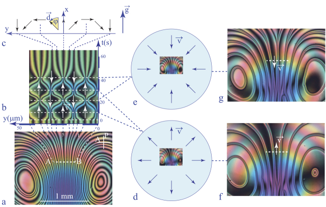
Figure 4.31. Action of an alternating Poiseuille flow on a wound up dowser field. (a) Stationary wound up dowser texture. (b and c) Spatiotemporal cross-section of the wound up dowser texture submitted to an alternating Poiseuille flow. (d and e) Diverging and converging radial Poiseuille flows driven by a harmonic modulation of the gap thickness. (f and g) Detailed views of the interference patterns
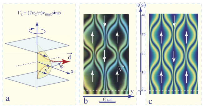
Figure 4.32. Simulation of the spatiotemporal cross-section. (a) Definition of the rheotropic torque. (b) Comparison of the experimental cross-section from Figure 4.31(b) with the simulation
In the presence of the alternating Poiseuille flow, trajectories of isogyres become wavy and one observes their association into π- and 2π-walls.
The 2π walls are first formed during the first half-period when the Poiseuille flow is directed upward in the direction of the x axis. When the flow is reversed, the 2πwalls split into π-walls that reassociate into new 2π-walls.
4.4.6.2. Analysis
In this experiment, the dowser field is submitted to four torques: the rheotropic, viscous, elastic and cuneitropic. The rheotropic torque has been introduced in section 4.4.1.2. When the Poiseuille flow v is parallel to the x axis (see Figure 4.31(c)), its expression is (see Figure 4.32(a)): Γrt = −αeff (vmax/h)sin φ with αeff = −2α2h/π. The viscous torque acting on the dowser field is given by the integral (see section 4.16.2):

with γeff = γ1h/2.
Similarly, the elastic torque is given by
with Keff = Kh/2. The cuneitropic torque, which will be discussed in more detail in the next section, is Γcunei = −(πKg)/h)sin φ.
The balance of torques acting on the dowser field leads to the following equation of motion:
For t ≤ 0, the dowser field is considered quasi-static in the absence of the alternating Poiseuille flow so that ∂φ/∂t = 0 and this equation is reduced to the balance of the elastic and cuneitropic terms. In section 4.5, we will see that its solution
describes a wound up phase field modulated by cuneitropism. The best fit with experimental data is obtained with Δφ = 0.33.
For t>0, this solution will be taken as an initial condition of equation [4.32], reduced to its viscous and rheotropic terms
with ![]()
Results of its numerical integration have been used for calculation of the intensity of light transmitted between crossed polarizers I = Iosin2[φ(y, t)]. The best fit with the experimental spatiotemporal cross-section in Figure 4.32(b) obtained with C = 0.25s−1 is plotted in Figure 4.32(c).
4.5. Cuneitropism, solitary 2π-walls
4.5.1. Generation of π-walls by a magnetic field
During discussions of 2π-walls generated by the rheotropic winding of the dowser field, we have shortly mentioned that, beside the rheotropic torque, the cuneitropic torque also contributes to their structure. Here, we will deal with the simpler case of solitary 2π-walls generated first by means of a rotating magnetic field and shaped later by the cuneitropism alone.
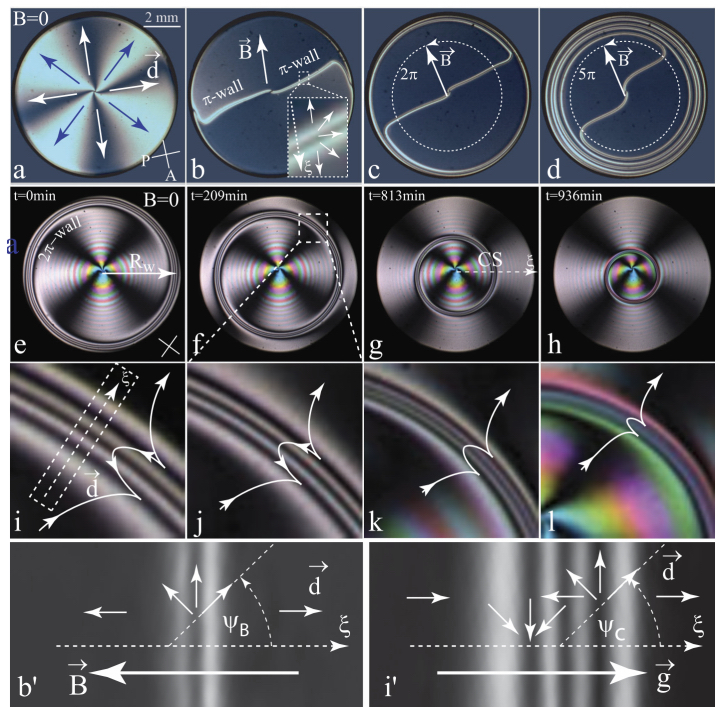
Figure 4.33. Winding of the dowser field by the magnetic field. (a) Initial radial dowser field. (b) Two π-walls generated by the magnetic field. (c and d) Configuration of the π-walls after rotation of the magnetic field by 2π and 5π. (e) Circular 2π-wall formed from 2 π-walls after suppression of the magnetic field. (f–h) Shrinking of the 2π-wall. (i–l) Detailed views of the 2π-wall. (b’–i’) Dowser fields in the π and 2π walls
A magnetic field B, parallel to the xy plane and applied to the radial dowser texture, deforms it into two π-walls as is shown in Figures 4.33(a) and (b). This deformation is due to the torque exerted by the magnetic field on the director n. As the thickness h is very small with respect to the magnetic coherence length ξm (see below), the z dependence of the director field inside the dowser texture is not affected by the magnetic field and can be expressed as a sum of two components, one parallel to the dowser field and the second one parallel to the z axis:

with θ = πz/h. After integration on z, we obtain:

with ψB corresponding to the angle between the dowser and magnetic fields.
In equilibrium, the shape ψB(ξ) (see Figure 4.33b’) of the π-wall satisfying the balance of the elastic and magnetic torques:
is given by
with

Let us mention that when the radial dowser field is submitted to the magnetic field, not only the two diametrically disposed π-walls are created. Due to the homeotropic anchoring conditions at the meniscus, the dowser field remains orthogonal to it. Therefore, at their junctions with the meniscus, the diametral π-walls split into pairs of peripheral walls parallel to the meniscus. These peripheral walls surrounding the whole droplet can be referred to as partial because the variation of the angle ψ across them is ![]() .
.
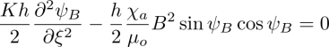
Figure 4.34. Slow elastic collapse of the circular 2π-wall. (a) Spatiotemporal cross-section extracted from a video along the line CS defined in Figure 4.33(g). (b) Variation of the width ξc of the 2π-wall with its radius Rw. Dots – experimental results; continuous line – fit to the theoretical prediction given in equation [4.46]
4.5.2. Generation and relaxation of circular 2π-walls
When the magnetic field starts to rotate slowly enough, the dowser field follows it and ΔψB starts to change (see Figures 4.33(c) and (d)). When after a whole 2π turn (Figure 4.33(c)) the magnetic field is suppressed, the dowser field relaxes into its radial configuration except for a circular 2π-wall that remains in the vicinity of the meniscus (see Figure 4.33(e)).
To recover the ground state, with the radial dowser field filling the whole droplet, about 20 h are necessary. During this very slow relaxation, this solitary circular 2π-wall shrinks (see Figures 4.33(e–h)). Simultaneously, the width ξw of the wall decreases (see Figures 4.33(i–l)).
An analogous behavior is observed when the slowly rotating magnetic field is suppressed after several whole 2π turns. For example, Figure 4.35 shows that four 2π-walls have been generated by this method. During the visco-elastic relaxation, these walls shrink simultaneously and collapse one after another.
4.5.3. Cuneitropic origin of the circular 2π-wall
The ground state radial configuration of the dowser field and the circular 2π-wall have the same origin – the cuneitropism (from the latin word cuneus = wedge). This phenomenon, also referred to as “geometrical anchoring” by Lavrentovich (1992), takes place when the limit surfaces are not parallel but form an angle γ. In such a wedge geometry, cuneitropism is a manifestation of the dependence of the distortion energy of the dowser texture on its azimuthal orientation with respect to the thickness gradient g =∇h.

Figure 4.35. Viscoelastic unwinding of the dowser field in a circular droplet can be seen as the shrinking and collapse of 2π-walls. Pictures taken at intervals of 80 min
To understand the coupling between the dowser field d and the thickness gradient g, let us consider first the dowser texture in a sample with a uniform thickness shown in Figure 4.36(a). Here, the director field n rotates by α = π between the limit plates separated by the distance h. In the approximation of the isotropic elasticity, the distortion energy per unit area is given by


Figure 4.36. Origin of the cuneitropism. (a and b) When h = constant, the distortion energy of the dowser texture does not depend on its azimuthal orientation. (c and d) In the wedge geometry, the distortion energy varies with the angle ψc between the dowser field d and the thickness gradient g
For symmetry reasons, this expression does not depend on the azimuthal orientation ψc of the dowser field d when the thickness is uniform.
When the upper plate is tilted by a small angle γ (Figure 4.36(b)), the director rotates between the limit surfaces by the angle α = π − γ cos ψc and the energy of the dowser state becomes
As γ cos ψc = g · d, we can say that the dowser field d couples linearly with the thickness gradient g. The resulting torque given by

tends to align d along the gradient g.
The shape ψc(ξ) of the 2π-wall (see Figure 4.33(i’)) results from the balance of the elastic and cuneitropic torques
By analogy with the π-wall discussed above, we have:
with

The width ξc of the 2π-wall should thus depend on the radius Rl because, in the sphere/plane geometry, the local thickness of the gap h as well as the tilt angle γ vary with the distance r from the center as

and
This theoretical prediction fits the experimental results plotted in Figure 4.34(b) well.
4.6. Electrotropism
4.6.1. Definition of the electrotropism
The rheotropism and cuneitropism discussed previously were due to linear couplings between the dowser field d and vectorial perturbations: the Poiseuille flow v and the thickness gradient g. Similarly, by definition, the electrotropism is a manifestation of a linear coupling of the dowser field d with the electric field E.
We will see below that the coupling of the dowser field with the electric field E (parallel to the (x,y) plane) is in practice more complex than linear because the dowser field d is submitted to the torque
exerted by the electric field E on the polarization P, which is a sum
of the spontaneous (flexo-electric) polarization (see section 4.6.2)
and of the anisotropic part of the polarization Pind induced by the electric field:
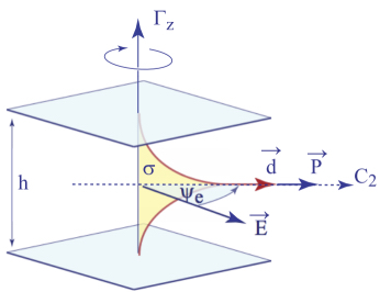
Figure 4.37. Spontaneous flexo-electric polarization of the dowser texture
Therefore, the detailed expression of the electric torque
also contains the second-order term due to the dielectric anisotropy of nematics. When the dowser field d makes an angle ψE with the electric field E, the electric torque can also be written as
We will see in the following that in experiments with wound up dowser fields, it is possible to detect both terms of this expression.
4.6.2. Flexo-electric polarization
Before that, it is important to emphasize that the spontaneous polarization of the dowser texture was expected from symmetry considerations similar to those of Meyer (1969) who announced, for the first time, the concept of the flexo-electricity and namely the linear relationship between distortions of the director field in nematics and the dielectric polarization (see equation [4.56]).
Indeed, as stated in section 4.1.3.3, the symmetry C2v of the dowser texture is so low that it allows for the existence of a spontaneous polarization Pfe parallel to the twofold axis C2, that is to say parallel to the dowser field: Pfe = Pfed (the subscript fe refers to the flexo-electric origin of the polarization).
Using the explicit expression of the director field
and the de Gennes’ definition of the polarization density (de Gennes and Prost 1993)
we can calculate the polarization per unit area of the dowser texture
with
Let us emphasize that this flexo-electric polarization of the dowser texture is independent of the gap thickness h.
4.6.3. Setup
The setup used for detection and measurement of the flexo-electric polarization is depicted in Figure 4.38. It is essentially the DDC1 device described in section 4.2.1 in which the glass slide is equipped with one of the four systems of transparent ITO electrodes shown in Figure 4.38(c).

Figure 4.38. Setup. (a) General perspective view. (b) Cross-section of the sample. (c) Systems of ITO electrodes
4.6.4. The first evidence of the flexo-electric polarization
The first evidence of the flexo-electric polarization of the dowser texture was obtained in experiments illustrated in Figure 4.39. They start with the synchronous winding of the dowser field discussed in section 4.4.2. After suppression of the excitation, the wound up dowser field reaches in a few seconds its quasi-equilibrium state with equally spaced black isogyres shown in Figures 4.39(a) and (d). Orientations of the dowser field indicated that these pictures have been detected by a transitory application of a divergent radial flow due to a small reduction of the gap thickness h. For example, in Figure 4.39(b) the orientation of the dowser field (white arrows) in enlarged isogyres is parallel to the Poiseuille flow (yellow arrows).
Subsequently, using the one-gap system of electrodes, an electric field has been applied to the wound up dowser texture. The formation of 2π-walls well visible in Figures 4.39(c) and (e) unveils the presence of the flexo-electric polarization in both MBBA (c) and 5CB (e). Let us note a crucial difference between these two pictures: in 5CB, the dowser field d in enlarged isogyres separating the 2π-walls is parallel to the electric field E, while in MBBA it is antiparallel to E. The conclusion is that the sign of the flexo-electric polarization Pfe = (π/2)(e3 − e1) is positive in 5CB and negative in MBBA.

Figure 4.39. The first evidence of the flexo-electric polarization in MBBA (a–c) and 5CB (d–e). (a and d) Wound up dowser texture in quasi-equilibrium. (c and e) 2π-walls induced by the electric field E. (b) Rheotropic detection of the wound up dowser field
4.6.5. Measurements of the flexo-electric polarization
Values of the flexo-electric polarizations in MBBA and 5CB have been measured in experiments (see Figure 4.40) performed with a weak enough electric field to neglect the contribution of the second-order term due to the dielectric anisotropy ɛa in equation [4.54]. They consist of measuring small deformations of the ground state radial configuration of the dowser field d submitted to an alternating electric field.
The ground state radial dowser field observed in polarized monochromatic light (see Figure 4.40(b)) displays an interference pattern made of isogyres (maltese cross) and isochromes (rings indexed N = 3,4,...). Upon application of a sinusoidal voltage U(t) = Uo cos(2πft) (f = 20 mHz) to the electrodes ITO1 and ITO2, we observe angular oscillations δα(t) of the black isogyres inside the ITO1/ITO2 gap. The orientation of crossed polarizers has been adjusted for a maximum intensity gradient dI/dα in the point P located in the middle of the ITO1/ITO2 gap (see Figure 4.40(d)). Oscillation δI(t) of the light intensity measured in P (see Figure 4.40(c)) is thus δI(t) = (dI/dα)δα(t). The intensity gradient dI/dα in P was determined from the plot I(α) in Figure 4.40(d). Knowing this, the angular oscillations of the dowser field δφ(t) = −δα(t) have been plotted in Figure 4.40(e). The same measurements of δφ(t) performed with 5CB are plotted in Figure 4.40(f).
It is obvious that oscillations δφ(t) of the dowser field have opposite signs in plots of Figures 4.40(e) and (f). The two schemes in Figures 4.40(g) and (h) show that in MBBA and 5CB the dowser field d is rotating, respectively, in anticlockwise and clockwise directions when, at t = 0, the electric field is antiparallel to the y axis.
Using the definition of the electric torque P × E, we obtain a confirmation of the result discussed above: in MBBA and 5CB, the flexo-electric polarization Pfe is, respectively, antiparallel and parallel to the dowser field d (see Figures 4.40(g) and (h)).

Figure 4.40. Measurements of the flexo-electric polarization in MBBA and 5CB. (a and b) The ground state radial configuration of the dowser field observed in white and monochromatic light. (c) Intensity of the transmitted light measured in point P. (d) Plot of the intensity measured along the circular path A-P-B. (e and f) Angular oscillations δφ of the dowser field inferred from variations of the intensity of light detected in point P. (g and h) Interpretation of the angular oscillations in terms of the electric torque Pfe ×E
The two plots in Figures 4.40(e) and (f) have another interesting feature: oscillations of the dowser field are shifted by π/2 with respect to the applied voltage U(t), that is to say to the electric torque driving them. This means that the restoring elastic and cuneitropic torques are negligible so that the equation of motion can be simplified as follows:
At the low frequency f = 20 mHz of the applied voltage, the electric field in the gap of width lg is generated in the so-called conductive regime for which Eo =Uo/lg. Then, the equation of motion results in
with

and the flexo-electric polarization is given by
With lg = 1 mm, Uo = 5 V (MBBA) or 3 V (5CB), γ1 = 100 mPa·s measured by Oswald et al. (2013) andh=31 μm measured from the interference pattern in Figure 4.40(b), we get
and
In the case of MBBA, the value of e3-e1 given in equation [4.63] agrees in sign and the order of magnitude with the result e3-e1 = -3.3 pC/m obtained for the first time by Dozov et al. (1982).
In the case of 5CB, the positive sign of e3-e1 is contrary to the result e3-e1 = −11 pC/m obtained by Link et al. (2001) from observation of 2π-walls. We will see below that electro-osmotic flows discussed in the following section contribute to the formation of the 2π-walls so they could be considered as a plausible reason for this disagreement.
4.7. Electro-osmosis
4.7.1. One-gap system of electrodes
An experiment performed with 5CB and illustrated by Figure 4.41 provides evidence of electro-osmotic flows in a wound up dowser texture submitted to a strong electric field. The general view of the wound up dowser texture in quasi-equilibrium in Figure 4.41(a) unveils the cuneitropic splitting of the isogyres’ pattern into 2π-walls discussed previously in sections 4.4.1.1 and 4.5. It allows us to identify orientations of the dowser field (white arrows) in enlarged black isogyres where it is parallel or antiparallel to the x direction.
This quasi-equilibrium wound up dowser field is then submitted to the electric field E = U/lg due to the voltage U(t) applied to the pair ITO1-ITO2 of electrodes separated by the gap of width lg = 0.3 mm. U(t) varies through time as follows:
![]()
The resulting evolution of the isogyres pattern is illustrated by the series of six pictures in Figure 4.41(b) as well as by the spatiotemporal cross-sections in Figures 4.41(c) and (e), which were extracted from a video along lines AB and CD defined in the picture labeled t1.
4.7.1.1. Effects due to the electric field inside the gap
In agreement with observations reported in section 4.6.4, the picture labeled t2 in Figure 4.41(b) shows that the electric field E inside the gap generates 2π-walls separated by strips in which the dowser field d is parallel to E. In a step-like reversal of the electric field, these 2π-walls split into pairs of π-walls moving apart (in the picture t3) until their recombine into new 2π-walls in the picture t4. Motions of the π-walls during this splitting-recombination process are clearly visible in the spatiotemporal cross-section of Figure 4.41(c). The existence of well-defined π walls is due to a large intensity of the electric field for which the second-order dielectric anisotropy term in equation [4.54] becomes significative. Their motion is another evidence of the role played by the first-order electrotropic term.
4.7.1.2. Effects due to the electric field outside the gap, evidence of electro-osmosis
Surprisingly, the isogyres’ pattern in Figure 4.41(b) is also affected by application of the voltage U(t) in areas outside the gap where the electric field vanishes. We will point out in the following that this is a manifestation of the electro-osmosis.
By definition, electro-osmosis refers to flows driven by forces exerted by the electric field on mobile charges in electric double layers at walls of a channel filled with a liquid. Let us suppose that in the experiment illustrated by Figure 4.41, the mobile charges at surfaces inside the gap are negative, as shown in Figure 4.42(c). The electric field E parallel to the x axis sets them in motion of velocity veo in the opposite -x direction.

Figure 4.41. Evidence of electro-osmotic flows. (a) General view of a quasi-equilibrium wound up dowser texture. (b) Formation and evolution of the π and 2π-walls in a strong alternating electric field. (c–e) spatiotemporal cross-sections taken along lines AB and CD defined in (a). (d–f) Numerical simulations (Pieranski and Godinho 2019a).
In a gap of infinite length, the flow would be plug-like v(z) = veo. However, as the gap has a finite width lg, the flow profile outside the gap must be parabolic, i.e. characteristic of Poiseuille flows. In virtue of the rheotropism, these Poiseuille flows of amplitude v(z = 0) = vPout outside the gap deform the equidistant isogyres’ pattern into 2π-walls separated by large strips in which the dowser field d is parallel to vPout.
4.7.1.3. Electro-osmotic effects inside the gap
In the absence of external forces, the Poiseuille flows outside the gap must be accompanied by pressure gradients ∂p/∂x shown in the scheme in Figure 4.42(e). As the directions of Poiseuille flows are the same on the left and right sides of the gap, there must be a pressure difference Δp between the two extremities of the gap. The plug flow inside the gap is thus accompanied by an adverse Poiseuille flow of amplitude v(z=0)= vPin driven by the pressure gradient Δp/lg.
In summary, inside the gap the deformation of the dowser field is due to a simultaneous action of two torques, the electrotropic and rheotropic ones:
with ![]()
From conservation of the global flow rate, we have
with
we obtain

Ceo (< 0 in 5CB) is the coefficient relating the velocity of mobile charges in the double layer to the electric field acting on them. Finally, the global torque due to the electric field can be written as
with
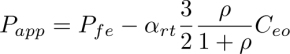
Figure 4.42. Poiseuille flows driven by electrosmosis in the one-gap system of electrodes. (a) Isogyres’ pattern deformed by application of the electric field. (b) Flow stream lines. (c) Flow profiles. (d) Cross-section of the nematic drop contained between the glass slide and the lens. (e) Pressure variation inside the drop
In 5CB, the second term is positive. If it is large enough, the apparent polarization can be positive even if the true flexo-electric polarization is negative.
4.7.2. Two-gap system of electrodes
The existence of electro-osmotic flows was confirmed in experiments with other systems of electrodes. In the system shown in Figure 4.38(c2), the two gaps, ITO1-ITO2 and ITO2-ITO3, can be connected either in series or in parallel.
In the case of the connection in series (see Figure 4.43(a)), the electric fields E in the two gaps have the same x direction so that, by symmetry, the x components of the global electro-osmotic fluxes Qx satisfy the following equality:
In the case of the connection in parallel (see Figure 4.43(b)), the electric fields E in the two gaps have opposite directions so that, by symmetry, we have
Due to the mirror symmetry of the droplet with respect to the (x,z) plane, we also have
Moreover, in the center (0,0) of the droplet where the thickness is minimal, the incompressibility condition takes the form
Using equations [4.72]–[4.74], we obtain:
which corresponds to a flow with a stagnation point SP(0,0) (see Figure 4.43(b)).
For these reasons, the isogyres’ pattern is equidistant in the stagnation point and the width ξ of the 2π-walls on the y axis decreases with the distance y from SP because the velocity |vyo| of the Poiseuille flow grows with y.
Let us also note that the isogyre enlarged by this flow parallel to the y axis is squeezed, in the middle of a 2π-wall, in adjacent gaps where the electro-osmotic flow takes the orthogonal direction, i.e. parallel to the x axis.

Figure 4.43. Electro-osmotic flows in the two-gap system of electrodes. (a) Gaps connected in series. (b) Gaps connected in parallel
4.7.3. Convection of the dowser field
As stated above, in the case of gaps connected in parallel, the Poiseuille flow on the y axis is parallel to it in virtue of equation [4.75]. For this reason, it not only generates the 2π-walls but also convects them. Indeed, the viscous term in the equation of motion of the dowser field, i.e. of the phase φ (see section 4.16.2), also contains in principle, beside the time derivative, the convection term:
The isogyres are orthogonal to the y axis so that the gradient ![]() is parallel to it. In the series case, the Poiseuille flow along the x axis is orthogonal to
is parallel to it. In the series case, the Poiseuille flow along the x axis is orthogonal to ![]() so that the convection term vanishes. On the contrary, in the parallel case, the Poiseuille flow and the gradient
so that the convection term vanishes. On the contrary, in the parallel case, the Poiseuille flow and the gradient ![]() are parallel so that the wound up dowser field is convected. All this is clearly visible in Figure 4.44 on spatiotemporal cross-sections taken along the line CS defined in Figure 4.43.
are parallel so that the wound up dowser field is convected. All this is clearly visible in Figure 4.44 on spatiotemporal cross-sections taken along the line CS defined in Figure 4.43.
In the series case (Figure 4.44(a)), trajectories of the isogyres are parallel to the time axis (except for the short splitting-recombination sequence due to the reversal of the voltage U).
In the parallel case (Figure 4.44(b)), the trajectories of the isogyres are skewed and the angle ∂y/∂t they make with the time axis increases with the distance y from the stagnation point SP. The sign of this angle changes upon the reversal of the voltage U because the direction of the electro-osmotic flows v is reversed.
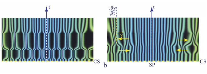
Figure 4.44. Convection of the dowser field. Spatiotemporal cross-sections along the line CS defined in Figure 4.43 (a) Gaps connected in series. (b) Gaps connected in parallel
4.8. Dowser texture as a natural universe of nematic monopoles
4.8.1. Structures and topological charges of nematic monopoles
In section 4.1.3.2, we stressed that the dowser texture is a natural universe of nematic monopoles because the +2π and −2π defects (called dowsons d+ and d-) of the dowser field are topologically equivalent to nematic monopoles. In other words, we could also say that dowsons are nematic monopoles embedded in the dowser texture.
The concept of monopoles as singularities of vector fields arises from the 19th-century works of Poincaré (1886). Their existence in nematics was postulated in 1972 by Nabarro (1972). As we have seen in section 4.1, nematic monopoles have also been considered by de Gennes in the first classification of defects in systems with order parameters resulting from broken symmetries (de Gennes 1972).
The general classification of monopoles in nematics is based on their topological charge defined by Kleman and Lavrentovich (2006) as the following integral over the surface of a sphere S2 enclosing them:

It is very instructive to calculate the topological charge of the so-called radial and hyperbolic monopoles represented in Figure 4.45. They occur, for example, alternatively on the axis of homeotropic cylindrical capillaries shown in Figure 4.4(b). Experiments have shown that two such adjacent monopoles attract each other, come together and finally annihilate.
One could think therefore, by analogy with electrostatic charges, that the topological charges of the radial and hyperbolic monopoles should be opposite and add to zero. Actually, this is a more subtle issue and we will discuss it below.
Let us start with the radial monopole (see Figure 4.45 “radial”) with the director field expressed in spherical coordinates (r, θ, φ) as
Its topological charge calculated from equation [4.77] isN=+1.

Figure 4.45. Continuous transformation relating the radial and hyperbolic configurations of the nematic monopole
Similarly, the director field of the hyperbolic monopole (see “hyperbolic” in Figure 4.45) can be written as
and its topological charge calculated from equation [4.77] is the same: N = +1.
The equality of topological charges of the radial and hyperbolic hedgehogs was understood and emphasized by Kurik and Lavrentovich (1988) who showed that structures of the radial and hyperbolic hedgehogs are connected by a continuous transformation, represented in Figure 4.45, and which analytically can be expressed as
with “the phase” ψo varying from zero (for the radial monopole) to π (for the hyperbolic monopole). Therefore, not only is there no difference in the topology of the radial and hyperbolic monopoles but also there exists a continuous set of structurally different monopoles having the same topological charge N = 1 (or N = -1). In fact, the set of structurally different monopoles is even larger than those defined by equation [4.80] because the symmetry with respect to the C∞//z axis is not necessary, as noted by Nabarro (1972).
In this context, the annihilation of a pair of the radial and hyperbolic monopoles occurring in capillaries appears to be paradoxical. To solve this paradox, let us note that the sign of the topological charge N, calculated from equation [4.77], is reversed upon the reversal n → −n of the director field. Therefore, if the sign of the director field in one of the monopoles of the pair is reversed, its topological charge becomes N = -1 and the sum of topological charges is zero as expected.
Reversal of the director field in one of the monopoles of the pair is in fact a necessity, as we will point out below using the example of a pair (d+, d-) of dowsons in the dowser texture.
4.8.2. Pair of dowsons d+ and d- seen as a pair of monopoles
Let us consider the dowser texture containing a pair of d+ and d- dowsons, i.e. a pair of the +2π and −2π disclinations of the two-dimensional dowser field d (see Figure 4.46). When they come in contact, their annihilation appears to be obvious from a topological point of view.

Figure 4.46. Pair of dowsons d+ and d- in the dowser texture. (a) View in polarized light; (b) The corresponding dowser field d
However, when the two defects are considered as monopoles in the three-dimensional director field n, their annihilation is more enigmatic in view of the former considerations. We must prove that the director field in one of the monopoles is reversed with respect to the configurations shown in Figure 4.45. For this purpose, let us consider the detailed views of the director field n inside the 2π wall connecting dowsons d+ and d- (see Figures 4.47(I) and (II)).
In the first case (I) of the clockwise 2π wall (rotation of the dowser field along the x axis), the defect labeled +2π(d+) has the structure of the radial monopole in 3D (see Figure 4.45), while the second −2π(d−) defect has the structure of the hyperbolic monopole (defined in Figure 4.45) with a reversed director field. For this reason, the total topological charge of this pair is zero.

Figure 4.47. The +2π and −2π defects (dowsons d+ and d-) of the dowser field d as monopoles of the director field n. (a) Top views showing a pair of dowsons d+ and din the dowser field d. The 2π walls in I and II have opposite winding directions. As a result, positions of dowsons are exchanged. (b) Lateral views of the director field n in the (y,z) plane. (c and d) Lateral views of the director field in the (x,z) plane. (e and f) Identification of topological charges of monopoles corresponding to dowsons d+ and d-
In the second case (II) of the anticlockwise wall, both defects d+ and d- have the structure of the hyperbolic monopole in 3D, with different orientations. The monopole corresponding to the −2π(d−) defect has its C∞ axis oriented in the x direction, while the C∞ axis of the second monopole has the z orientation. Let us stress that the director field of the second monopole is reversed with respect to the first so that its topological charge is -1 and the total charge of the pair is zero again.
We will come back to the discussion of the annihilation of pairs of monopoles in section 4.10 first but we must explain how monopoles are generated.
4.8.3. Generation of monopole–antimonopole pairs by breaking 2π-walls
In section 4.1, we gave an explanation of the scarcity of monopoles in nematics. Namely, the director field on a sphere surrounding a monopole mapped on the space of the nematic order parameter (projective plane equivalent to one hemisphere) covers it twice; and such a complex configuration of the director field can hardly occur spontaneously during the isotropic ⇒ nematic transition.
In section 4.8.3.2 we will show that, on the contrary, the configuration of the director field in 2π-walls in a wound up dowser texture is so close to that of monopoles that an adequate perturbation can result in the generation of monopoles. To be more precise, we must say the generation of monopole–antimonopole pairs because generation of a single monopole is precluded for topological reasons.
4.8.3.1. Generic experiment
Before that, let us describe first a typical experiment, illustrated by Figure 4.48, in which such monopole–antimonopole pairs are generated. It starts by the synchronous winding of the dowser field in the DDC1. This process was described in detail in section 4.4.2. Here, the winding process is illustrated by a series of seven pictures (a–g). It starts from the quasi-static radial texture with the residual monopole located off the center. The direction of the 2π-wall indicates that the residual monopole, located at its extremity, is shifted to the right.
Six subsequent pictures show that six new 2π-walls are generated by the up-and-down motion s(t) of the glass slide.
The next and last move of the slide is directed downward, more rapid and has a larger amplitude so that the width ξrt of the 2π-walls is strongly reduced, as shown in the eighth picture (Figure 4.48(h)).
The next two Figures 4.48(i) and (j) show the broken walls during relaxation after cessation of flows. Using the convention introduced in section 4.1.3.2, the monopoles and antimonopoles are labeled as +2π and −2π. Their identification results from the detailed analysis of the isogyres’ pattern. As an example, we show in Figure 4.48(k) a detailed view of the dotted rectangle from the picture 4.48(j). Orientations of the dowser field met along the anticlockwise circuit surrounding the extremity of the 2π-wall are redrawn in the picture (Figure 4.48(l)). Their rotation in the opposite clockwise direction is the fingerprint of the antimonopole -2π.

Figure 4.48. Generation of monopole–antimonopole pairs. (a) Radial dowser field. (b–g) Generation of six 2π-walls. (h) Thinning of 2π-walls by a rapid Poiseuille flow results in them breaking. (i–j) Relaxation of the dowser field after cessation of flows. (k) Identification of the dowser field along an anticlockwise circuit surrounding an antimonopole. (l) Corresponding clockwise rotation of the dowser field
4.8.3.2. Topological relationship between 2π-walls and monopoles
In Figure 4.49, we show another example of the generation of monopole–antimonopole pairs through the rheotropical thinning and breaking of 2π-walls. The generation process is resolved in time in pictures a1–a6. Picture b shows a detailed view of the dotted rectangle defined in a1. The dowser field d, drawn with white arrows, has been inferred from the pattern of isogyres.
The four schemes in Figure 4.49(c) show perspective views of the director field in a dowser texture. They are labeled from 0◦ to 270◦ because their director field, when mapped on the sphere in d, forms meridians with these longitudes. For example, the director field from the scheme labeled 0° is mapped on the prime meridian 0◦. Clearly, the director field from the (y,z) cross-section of one 2π wall covers the whole sphere once. As the space of the nematic order parameter corresponds to one hemisphere, the director field from the (y,z) cross-section of one 2π wall covers it twice, once on the whole North hemisphere and the second time on the whole South hemisphere.
Let us recall that, as stated already in section 4.1.1.3, the director field on a sphere surrounding a monopole also covers the space of the nematic order parameter twice. In the present case of monopoles and antimonopoles located at extremities of a broken 2π-wall, we should rather consider the director field on a cylinder surrounding the monopole or the antimonopole. This property is illustrated once again in Figure 4.49(d) labeled “monopole”. In the case of the antimonopole, this is also true. The only difference is that during the mapping following the dotted circuit oriented West, the sphere of the order parameter is covered in the opposite east direction.
We can thus say that the director fields (1◦) on a (x,z) cross-section of a 2π-wall and (2◦) on a cylinder surrounding a monopole (or antimonopole) are topologically equivalent.
4.8.3.3. Conjecture on the rheotropic breaking of 2π-walls
During generation of pairs of monopoles (see Figures 4.48 and 4.49), segments of 2π-walls are replaced by a homogeneous dowser field texture oriented in the direction of the Poiseuille flow. From the point of view of the energy balance, on the one hand, the gain of the elastic energy is proportional to the segment’s length L of the suppressed wall of tension τrt: ΔEwall=-τwallL. On the other hand, there is an energy expense corresponding to the total energy of the two defects: ΔEM+AM =EM +EAM.
Let us first estimate the energy gain. During the rheotropic generation process, the 2π-walls of the wound up dowser field are thinned by the Poiseuille flow of amplitude vo. From the balance of the elastic and rheotropic torques:

we get
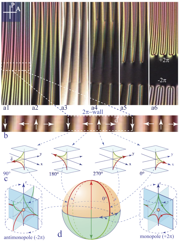
Figure 4.49. Topological relationship between 2π-walls and monopole–antimonopole pairs. (a) Time resolved generation of monopole–antimonopole pairs. (b) Detailed view of the dowser field in the dotted rectangle defined in the picture a1. (c) Perspective views of the director field inside the 2π-wall. (d) Mapping of the director field from the 2π -wall onto the space of the nematic order parameter
with the thickness of the wall

which decreases with the flow velocity vo.
The elastic energy per unit length of a 2π-wall of width ξrt or equivalently its tension τwall given by the integral
is inversely proportional to the wall width ξrt or, using expression [4.83], proportional to ![]() In conclusion, the energy gain from suppression of a segment of a 2π-wall grows as L
In conclusion, the energy gain from suppression of a segment of a 2π-wall grows as L ![]() .
.
The energy loss depends on the configuration of the generated monopoles, radial or hyperbolic, and given as (see the review article on point defects by Kleman and Lavrentovich (2006)):
with R corresponding to the size of their volume. In statu nascendi, the size R is of the order of ξrt/2.
Using equations [4.85] and [4.84], we finally obtain:
The critical thickness corresponding to ΔE = 0 is then given as
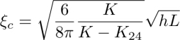
As the critical thickness decreases with the length L of the destroyed segment of the 2π-wall, we could think that the 2π-wall is unstable with respect to generation of dowsons pairs.
This result is contrary to experimental facts reported above. However, we still do not know what the detailed mechanism is of the wall destruction→ dowsons’ pair generation process. If it is a continuous transformation with some energy barrier (per unit length of the wall) to overcome, the 2π-wall would not be unstable but only metastable with respect to the generation of dowsons pairs.
4.9. Motions of dowsons in a wound up dowser field
4.9.1. Single dowson in a wound up dowser field
The energy balance given in equation [4.86] still holds after generation of the dowsons’ pair and, in this context, it has another meaning confirmed by observations: dowsons are moving apart because the energy ΔE decreases when the distance L between dowsons grows.
When the distance L is much larger than the width ξwall of the wall, the dowsons d+ and d- of the pair become independent and their motion inside the wound up dowser field can be analyzed separately.
For example, we show in Figures 4.50 and 4.51 the simplest case of one dowson d+ embedded in the dowser field wound up by means of the Dowsons Collider 2, discussed in section 4.4.3 and shown again in Figure 4.50(a).
Due to the structure of the DDC2 device, the distribution of the rheotropic torque produced by it is antisymmetric with respect to the reflection in the (x,z) plane (see Figure 4.50(b)) and the phase gradien ![]() on the x axis is orthogonal to it. In polarized light, this last feature of the wound up dowser texture is obvious in Figure 4.50(c): isogyres (which are lines of constant phase) are parallel to the x axis.
on the x axis is orthogonal to it. In polarized light, this last feature of the wound up dowser texture is obvious in Figure 4.50(c): isogyres (which are lines of constant phase) are parallel to the x axis.
The solitary dowson d+ is indicated in Figure 4.50(c) by an arrow, while in Figure 4.50(d) it is located in the dotted rectangle. As the picture in Figure 4.50(d) was taken 380 s after the picture in Figure 4.50(c) , it is obvious that the dowson is moving along the x axis.
The motion of the dowson d+ is illustrated in more detail in Figure 4.51. First of all, the series of five pictures a–e shows successive positions of the dowson at t = 0, 380, 520, 620 and 700 s. These pictures also show that the local wavelength λ of the wound up dowser field varies with the x position of the dowson.
These pictures were extracted from a time-lapse video containing 55 pictures taken at intervals of 20 s. Using all of them, the velocity v = dx/dt and the width ξwall = λ of the wall, terminated by the dowson, were measured and plotted as red crosses in Figure 4.51(f). Clearly, the velocity of the dowson depends on λ. Moreover, as on this log-log plot, the experimental points seem to be aligned on a line, they were fitted to the power law v ∼ λα with the best fit obtained for α=-1.24.
Figure 4.50. Motion of a dowson d+ in a dowser field wound up in the Dowsons Collider 2. (a) Scheme of the Dowsons Collider 2. (b) Distribution of the rheotropic torque. (c and d) Isogyres pattern of a wound up dowser field with one dowson d+
4.9.2. The Lorentz-like force
The motion of the dowson d+ is driven by the tension τwall of the wall to which it is attached. In the absence of flows and in quasi-equilibrium, the phase φ of a wound up dowser field must satisfy equation [4.81] reduced to the elastic torque alone. In two dimensions (x,y), it takes the form
In the vicinity of the x axis, its solution

involves the wavelength λ(y) resulting from the winding process.
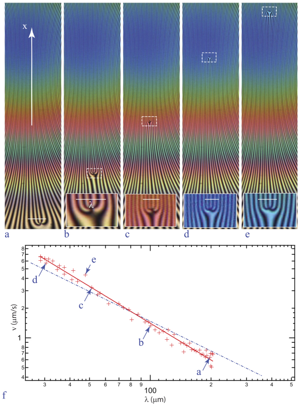
Figure 4.51. Motion of a dowson d+ in a dowser field wound up in the Dowson Collider 2. (a–e) Pictures taken at t = 0, 380, 520, 620 and 700 s. (f) Plot of the dowsons’ velocity versus the width λ of the 2π-wall to which it is attached. Crosses – experimental data. Dotted line – the 1/λ dependence expected from equation [4.96]. Red line – the best fit to the power law v ∼ λα with α = −1.24
The elastic energy per unit length of the 2π-wall (or equivalently its tension τwall) is given by the integral

Figure 4.52. Lorentz force on a vortex in superconductors and on a dowson in the dowser texture. (a) Phase singularity of a vortex or of a dowson. (b) Phase gradient due to the transport current in a superconductor or to the winding of the dowser field. (c) Lorentz force proportional to 
The corresponding force acting on the dowson is proportional to the phase gradient ![]() and is orthogonal to it so that it can be alternatively expressed as
and is orthogonal to it so that it can be alternatively expressed as

Where ![]() is a unit vector parallel (or antiparallel) to the z direction.
is a unit vector parallel (or antiparallel) to the z direction.
In terms of the classification proposed by de Gennes (see section 4.1), dowsons are similar to vortices in two-dimensional superconductors because they both correspond to Δφ = 2π defects of the phase field φ(x, y). In the presence of a current density ![]() vortices are submitted to the Lorentz force:
vortices are submitted to the Lorentz force:
exerted by the current density ![]() on the quantified magnetic flux
on the quantified magnetic flux ![]() of the vortex. Knowing that the current density is proportional to the phase gradient:
of the vortex. Knowing that the current density is proportional to the phase gradient:

we obtain:
We can now conclude that the force acting on a dowson in a wound up dowser texture, given by equation [4.91], is analogous to the Lorentz force exerted by the density current on vortices in superconductors, given by equation [4.94].
4.9.3. Velocity of dowsons in wound up dowser fields
During the motion of a dowson with velocity v, the driving tension of the wall τwall (or the Lorentz force), given by equation [4.91], is opposed by the force τvisc resulting from the viscous dissipation, which can be estimated as:
From the balance of forces, we obtain:

The 1/λ dependence of v(λ) is plotted in Figure 4.51 with the dotted line. As mentioned above, the experimental data are better fitted with the power law v ∼ λ−1.24. A plausible cause of this disagreement is that, as we point out below, the force fd acting on a dowson inserted in a wound up dowser field can differ from the Lorentz force ∼ 1/λ (equation [4.92]) calculated above.
4.9.4. The race of dowsons
The second piece of evidence of the deviation from the fd ∼ 1/λ dependence came from an experiment called “the dowsons’ race” (see Figure 4.53), which starts by the rheotropic breaking (see section 4.8) of a large set of adjacent 2π-walls in a wound up dowser field, shown in Figure 4.53(a). By this means, we obtain two sets of dowsons d+ and d- aligned on two lines, as in Figure 4.53(b). Pulled by tension of walls to which they are attached, dowsons d+ and d- start, att=0s,tomove in opposite directions. Let us follow the motion of two adjacent dowsons d+ indicated by arrows and labeled d1 and d2 in Figure 4.53(b). At the beginning of the race, velocities of all dowsons d+ are the same in order that they remain aligned on one moving line. In particular, after 19 s of the race, dowsons d1 and d2 are still running side by side.
Surprisingly, a dozen seconds later an instability occurs: the set of running dowsons is divided into two subsets, which could be called “slow” and “fast”. Therefore, in picture d, taken at t = 78 s, the slow dowson d1 is behind the fast dowson d2. In the next two pictures, taken at t = 183 s and 337 s, the gap between d1 and d2 becomes larger.

Figure 4.53. The dowsons’ race. (a) Dowser texture wound up in the DDC2 device. (b) At t = 0, two sets of dowsons d+ and d- generated rheotropically (see section 4.8) start to move in the opposite direction. (c–f) Pictures taken at t = 19, 78, 183 and 337 s (collaboration with Hadjiefstatiou and Montagnat (2017))
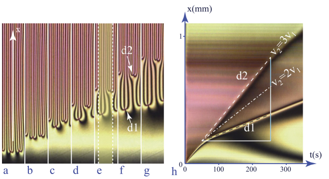
Figure 4.54. Race of dowsons. (a–g) Pictures taken at intervals of 20 s. (h) Spatiotemporal cross-section
Other features of the race are illustrated in Figure 4.54. The series of pictures a–g gives a more detailed view of dowsons d1 and d2. On the spatiotemporal cross-section extracted, along the strip defined in Figure 4.54(e), from a video recorded at rate of 1 frame/s, trajectories of dowsons d1 and d2 are well visible. Initially, they coincide but after about 50 s they separate. Velocity v2 of the dowson d2 is about three times larger than that of the dowsons d1, i.e. v1. The trajectory of the dowson d2 with the velocity expected from the Lorentz force ∼ 1/λ alone, v2= 2v1, is also plotted with a dash dotted line. The explanation of the observed v2=3v1 dependence instead of the expected one, v2=2v1, involves the calculation of the gain in the elastic energy due to the motion of slow and rapid dowsons. Four schemes in Figure 4.55 are useful for a straightforward understanding of the discussion. Three colors, gray, blue and yellow, represent three levels of the elastic energy density: E = 0 – gray, Eλ = (Kh/2)(2π/λ)2 – blue and Eλ/2 = (Kh/2)[2π/(λ/2)]2 – yellow.
Displacement Δx of a slow dowson lowers the elastic energy by

The force driving the motion of the slow dowson is thus

Figure 4.55. Estimation of forces driving the motion of dowsons involved in the race. (a and b) Slow dowsons. (c and d) The most rapid dowsons
The rapid dowsons of width λ/2 are inserted between the 2π-walls of the slow dowsons. Therefore, there are two contributions to the gain of the elastic energy. From the scheme c in Figure 4.55(c), we have

which generates the force 2Fλ.
The second contribution comes from the additional elastic relaxation in gray areas left by the displacement of the rapid dowson. Here, the gain in elastic energy is
which generates the force Fλ.
The total force acting on the rapid dowson is thus
so that, by virtue of equation [4.122], its velocity is three times larger than that of the slow dowson, as observed.
4.9.5. Trajectories of dowsons observed in natural light
Almost all experiments with the dowser texture were done with Dowsons Colliders equipped with crossed polarizers, as patterns of isogyres and isochromes are very helpful for interpretation of results. Isochromes allow us to measure the local thickness and visualize its gradients. Isogyres allow us to monitor the process of the phase winding or to identify the type of defect, d+ or d-, embedded in the wound up dowser field. In other words, because of the optical anisotropy of nematics, the phase φ of the complex order parameter eiφ is an observable quantity.
The importance and abundance of information that can be inferred from these interference patterns in polarized light becomes obvious when we deal with results of experiments with the dowser texture observed in non-polarized light, or if we examine results of experiments with vortices in superconductors imaged with a scanning tunneling microscope. In both cases, the phase in not an observable quantity and only the core of dowsons or vortices (Embon et al. 2017) can be distinguished.
For example, Figure 4.13 was obtained by superposition of images taken without polarizers. In this composite picture, dowsons appear as blueish dots that form dotted lines corresponding to trajectories of dowsons d+ and d-. These trajectories lead to collisions of dowsons pairs indicated by circles drawn, respectively, with solid or dashed lines when annihilation or passing-by occurs.
The second example of such a composite picture is given in Figure 4.56(a). Here, all trajectories of dowsons in the DDC2 setup start at the moment of generation of dowsons pairs. Annihilation of dowsons’ pairs, taking place on dashed lines, can be easily identified. The instability of the dowsons’ race discussed above is also well visible.
The third example, given in Figure 4.56(c), concerns trajectories of dowsons in the DDC2 setup during the asynchronous winding of the dowser field. Arrows indicate their starting points at t = 0, corresponding to the beginning of the winding. The most striking feature of these trajectories is their spiral shape indicating that dowsons circulate around the maximum C of the winding angular velocity ω(x, y) and simultaneously move away from it.
The second significative feature is that the dowson d- indicated by a larger arrow stays in the vicinity of its starting point for a long time, located at the maximum of the angular velocity ωmax. These those will be confirmed by those made with polarized light.

Figure 4.56. Trajectories of dowsons in the DDC2 setup recorded in non-polarized light. (a) Generation and annihilation of dowsons’ pairs. The dowsons’ race instability is also well visible. (b) Trajectories of dowsons during the winding process. Note that the dowson d- indicated by a larger arrow stays in the vicinity of its starting point for a long time
4.9.6. Trajectories of dowsons observed in polarized light
4.9.6.1. Gyrophilic behavior of dowsons d-
Indeed, such “gyrophilic” behavior of dowsons d- is confirmed in the experiment illustrated by Figure 4.57. Here, two dowsons d- are located at the two extrema of the angular velocity and remain there during the winding. Other dowsons are going away and possibly annihilate by pairs, as indicated by the circles.
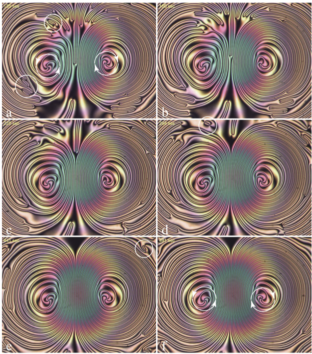
Figure 4.57. Gyrophylic behavior of dowsons d- during phase winding with the DDC2 setup. Two dowsons d- located in the vicinity of the extrema of the angular velocity of winding stay there. Their maltese cross-like isogyres patterns are rotating with angular velocities ωmin and ωmax. Other dowsons, going away, annihilate by pairs indicated by the circles

Figure 4.58. Gyrophylic behavior of dowsons d- during the phase winding with the CDC2 setup. Beside the dowson d- trapped at the maximum of the angular velocity ωmax several other dowsons d- are trapped in the annular minimum ωmin of the angular velocity
Let us stress the isogyres’ patterns present, in these pictures, taken in polarized light allow us to easily identify dowsons d+ and d-. Moreover, they also allow for measuring the angular velocities ωmin and ωmax because the maltese cross-like isogyres of dowsons d- are rotating with these velocities.
The gyrophilic behavior of dowsons d- is confirmed in the experiment carried out using the Circular Dowsons Collider 2 and illustrated by Figure 4.58. Here, beside the dowson d- trapped at the central extremum of the angular velocity ωmax several other dowsons d- are trapped in the second, annular extremum ωmin of the angular velocity. The maltese crosses of the central and the peripheral dowsons are rotating, respectively, in opposite anticlockwise and clockwise directions as expected.
4.9.6.2. Gyrophobic behavior of dowsons d+
The gyrophilic behavior of dowsons d- is confirmed once again in the experiment made using the CDC1 and illustrated by Figure 4.59. Here, at the beginning of the winding four dowsons d+ and three dowsons d- are embedded in the dowser field. The dowson d- located initially in the vicinity of the extremum ωmax is attracted to it and stays there as expected.
This experiment also shows that two dowsons d+ located initially in the vicinity of the extremum ωmax have a gyrophobic behavior: they are going away during the winding. Other dowsons more distant from ωmax annihilate by pairs.
The gyrophobic behavior of dowsons d+ is obvious in the experiment illustrated by Figure 4.60. Here, the dowser field contains only one dowson d+, which is called residual because its presence is necessary for topological reasons inside the droplet with homeotropic boundary conditions. In Figure 4.60(a) it is located in the vicinity of the gap center. During the winding, Figures 4.60(b–d) show that new loop-like isogyres are generated at the maximum of the angular velocity of the winding which, as shown in the insert, is located in the gap center. Colloquially speaking, the dowson d+ is pushed away by expanding isogyres loops.
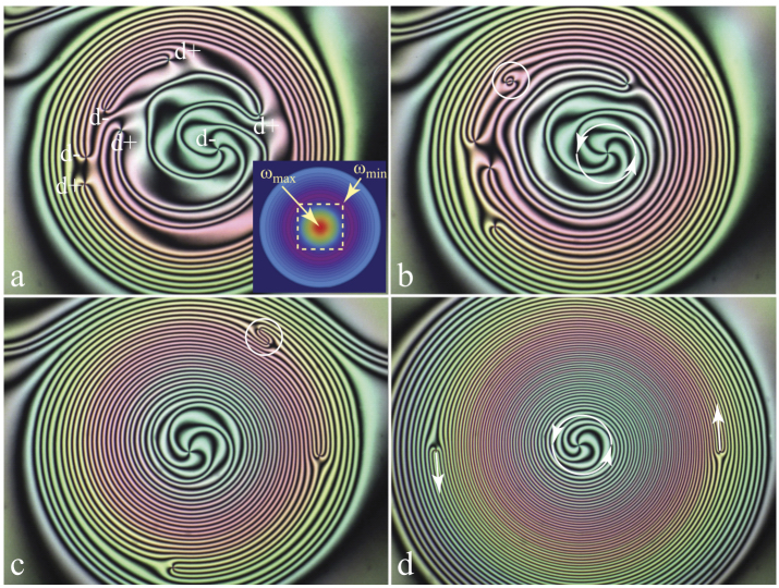
Figure 4.59. Gyrophobic and gyrophylic behaviors of dowsons. (a) Four dowsons d+ and three dowsons d- embedded in the dowser field during winding. (b and c) Annihilation of two dowsons pairs. (d) The stationary Cladis–Brand 2 state with the dowson d- at the maximum of the angular velocity of winding, and two dowsons d+ orbiting around it
4.9.6.3. Gyrophobic behavior of dowsons d+
Explanation of the gyrophobic behavior of dowsons d+ is done graphically in Figure 4.61(I). When a dowson d+ (scheme a) is inserted in a defect-less wound up dowser field (scheme b) in the point with φins = 0, a 2π wall is created (scheme c). The detailed view of the inserted dowson shows that it has the same configuration as in (a). However, when the phase of the insertion point is φins = −π/2 (scheme f), the detailed view of the inserted dowson (scheme h) shows that its configuration changed with respect to the one in the scheme d. This means that the configuration of the dowson d+ changes when the insertion point moves in the direction of the phase gradient or, alternatively, if the wound up dowser field moves across the inserted dowson. Now, the elastic energy E(φins) of the dowson d+ depends, via φins, on its configuration which in polar coordinates (r, φ) is given by
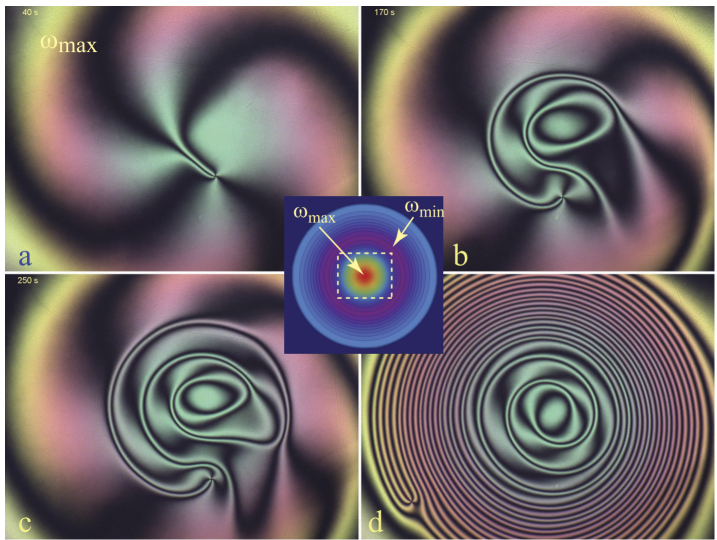
Figure 4.60. Gyrophobic behaviors of dowsons d+. (a) The residual dowson d+ located in the vicinity of ωmax. (c and d) During the winding it goes away as if it was pushed by isogyres generated at ωmax. (d) The stationary Cladis–Brand 1 state
On the basis of symmetry arguments, the function E(φins) can be written as a Fourier series limited to cosine terms:
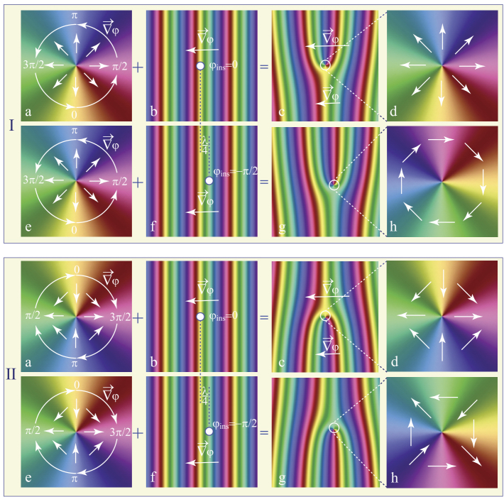
Figure 4.61. Gyrophobic and gyrophylic behaviors of dowsons. (I) Dowson d+. (II) Dowson d-. (a) Dowser fields d and φ. (b–f) Defect-less wound up dowser field. (c–g) Wound up dowser fields with the dowson inserted in them. (d and h) Detailed views of the inserted dowson. Its configuration depends on the phase φins in the insertion point defined in (b) and (f)
In Figure 4.62, we plotted the pertinent part of this expression
with B/A=0.75 estimated from experiments discussed in Pieranski et al. (2016b). This function has two minima in which the configuration of the dowson d+ is close to the clockwise and anticlockwise circular ones. In conclusion, the gyrophobic behavior of d+ dowsons results mainly from the existence of an absolute maximum, which acts as an energy barrier to overcome when φins varies. At this absolute maximum, the dowser field has the outward radial configuration, which in 3D corresponds to the hyperbolic configuration of the monopole.
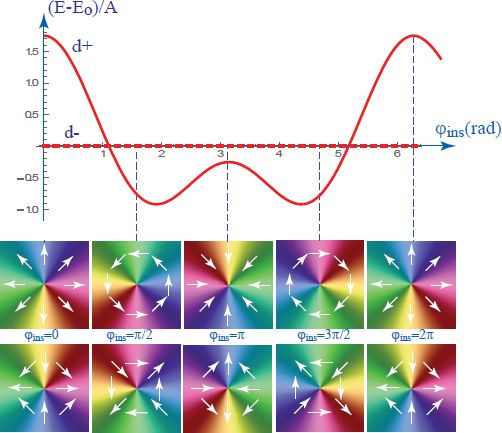
Figure 4.62. Variation of the energy of dowsons and of their configurations with the phase of the insertion point φins
4.9.6.4. Gyrophilic behavior of dowsons d-
The case of the d- dowson is represented in Figure 4.61(II). When the insertion point varies from φins = 0 to φins = −π/2, the field d in the vicinity of the dowson rotates as a whole by π/4, which does not change the elastic energy. One could think therefore that the behavior of the dowson d- should be rather neutral with respect to changes of the phase φins = 0.
In reality, it is more complex because, as shown in Figures 4.57–4.59, dowsons dcan be trapped in extrema of the angular velocity. So far no satisfactory explanation of this experimental fact has been found.
4.9.6.5. Stationary Cladis–Brand states
The gyrophobic and gyrophilic behaviors of dowsons are at the origin of stationary states occurring during the winding of the dowser field. We call them Cladis–Brand 1 and Cladis–Brand 2 with the aim of emphasizing their similarity with an analogous stationary state, discovered previously in Smectic C free-standing films (Cladis et al. 1995).
They have been already mentioned above but we show them again in Figure 4.63 with additional details, useful for discussion. During the asynchronous winding process in the CDC1 setup, the maximum of the angular velocity ω = dφ/dt = ωmax is located in the center of the gap. We can consider this maximum as a phase source, that is to say a point in which the phase is created at the rate dφ/dt = ωsource. During the winding, the phase growth rate ωsource decreases because the rheotropic torque is opposed by the growing elastic torque.
This phase source is surrounded by a circle, drawn in the insert with a dashed line, on which ω = 0.
Let us consider first the case of the CB1 state. It occurs when the dowser field at the beginning of winding contains only one gyrophobic dowson d+. As discussed previously, during the winding, the dowson d+ remains at the edge of the wound up dowser field and, pulled by the 2π-wall, is orbiting, with some period T, around the phase source. Such an orbiting dowson d+ acts as a phase sink absorbing the phase at the rate ωsink = −2π/T, which grows in time because the width λ of the wall decreases.
The stationary state φ(x, y, t)CB1 is reached when
The spatiotemporal cross-section in Figure 4.63(c), extracted from a video along the line CS, gives a graphical demonstration of this equality. It shows that during one period T = 30 min four new isogyres are created at the source in the center and four isogyres are lost when the dowson d+ crosses the line CS.
In the case of the CB2 state, four isogyres are created, every 21 minutes, at the center by one whole turn of the maltese-cross, and four isogyres are lost when one of the dowsons d+ crosses the line CS.
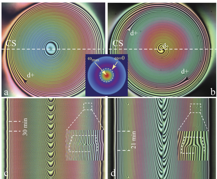
Figure 4.63. Cladis–Brand stationary states. (a) C-B1 state: dowson d+ orbiting around the phase source in the center. (b) C-B2 state: two dowsons d+ orbiting around the dowson d- rotating in the center. (c) Spatiotemporal cross-section of C-B1. (d) Spatiotemporal cross-section of C-B2
4.10. Collisions of dowsons
Collisions of dowsons have already been mentioned during discussions concerning Figures 4.13, 4.56(a), 4.57 and 4.59. In particular, Figures 4.13 and 4.56(a), obtained by superposition of images taken at intervals of a few seconds, showed trajectories of dowsons leading to collisions. Another example of colliding trajectories is shown in Figure 4.64. Figures 4.13, 4.56(a) and 4.64 show the two alternative outcomes of collisions: an annihilation indicated by circles drawn with a solid line or an avoidance indicated by circles drawn with a dashed line. Using the vocabulary of atomic or elementary particles physics, we can ask: What is the annihilation cross-section of dowsons’ pairs?

Figure 4.64. Trajectories of dowsons leading to collisions of dowsons’ pairs obtained by superposition of pictures taken at intervals of 5 s. Starting points of dowsons d+ and d- are indicated with yellow and blue arrows, respectively. Collisions resulting in an annihilation of a dowsons’ pair are indicated by solid line circles, and those leading to an avoidance are indicated by dashed line circles
4.10.1. Pair of dowsons (d+,d-) inserted in a wound up dowser field
In the search for the answer, let us consider two other examples of collisions, shown in Figure 4.65. These pictures, taken in polarized light, contain information about the dowser field, which is missing in images obtained without polarization. They suggest that the outcome of collisions depends on the distance of trajectories in terms of the phase difference Δφ.
When a pair of dowsons d+ and d- is inserted at points (x±,y±) in a dowser texture wound up in y direction, the phase field can be expressed as

When the two dowsons are far away, i.e. when |x+ − x−| ![]() λ, they move on linear trajectories defined y(t) = y+ and y(t) = y−. The linear distance between these trajectories is thus
λ, they move on linear trajectories defined y(t) = y+ and y(t) = y−. The linear distance between these trajectories is thus
while in terms of the phase the distance is
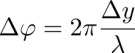

Figure 4.65. Collisions of dowsons’ pairs. (I) Avoidance, (II) Annihilation: (a) The dowser texture wound up in the CDC1 setup. (b–e) Images taken at intervals of 25 s
For example, in Figure 4.66(a–g), the phase difference Δφ varies between 0 and 3π.
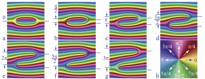
Figure 4.66. Collisions of dowsons embedded in a wound up dowser field. Their distance in terms of the phase difference Δφ varies from 0 in (a) to 3π in (g). The color code for the phase field is given in (h)
By comparing these pictures with those in Figure 4.65, we can say that in the case of the avoidance in Figure 4.65(I), the phase difference Δφ is of the order of 3π/2 while in the case of annihilation in Figure 4.65(II), it is Δφ ≈ π/2.
4.10.2. Cross-section for annihilation of dowsons’ pairs
Statistical study of collisions of pairs of dowsons d+ and d- in wound up dowser textures lead us to the conclusion that their issue depends on the distance Δφ of trajectories and, more precisely, there exists a critical phase difference Δφc = π such that:
- 1) for |Δφ| > Δφc, the avoidance occurs;
- 2) for |Δφ| < Δφc the annihilation takes place;
- 3) for |Δφ| = Δφc the outcome of the collision is random.
In other words, we can say that the annihilation cross-section is Δφc = π in terms of the phase or, equivalently, Δyc = λ/2 in terms of the linear distance.
4.10.3. Rheotropic control of the collisions outcome
The rules, stated above, are valid only for collisions occurring in quasi-static or stationary wound up dowser fields with a homogeneous phase gradient
![]() Now, we know from section 4.4.6 (see Figure 4.31) that Poiseuille flow splits a wound up dowser field into 2π-walls. We will show below that in the case of a dowson pair coming to a collision, this action of the Poiseuille flow can alter the issue of the collision.
Now, we know from section 4.4.6 (see Figure 4.31) that Poiseuille flow splits a wound up dowser field into 2π-walls. We will show below that in the case of a dowson pair coming to a collision, this action of the Poiseuille flow can alter the issue of the collision.
Let us consider the example of the dowsons’ pair in Figure 4.67. The phase field represented in Figure 4.67(a) has been calculated using equation [4.106] with (x+,y+) = (−5, −π/4) and (x−,y−) = (5,π/4) so that

Figure 4.67. Action of a Poiseuille flow on the outcome of a collision. (a) Dowsons’ pair inserted in a quasi-static wound up dowser field. (b) Generation of 2π-walls by a Poiseuille flow v in x direction. (c) Generation of 2π-walls by a Poiseuille flow v in -x direction
In terms of the collision rules formulated above, an annihilation of this dowsons pair is granted.
Application of the Poiseuille flow in the x direction perturbs the field φo(x, y) as shown in Figure 4.67(b): a narrow 2π-wall is now connecting the two dowsons. Obviously, pulled by this wall, the dowson will rapidly come into a collision and the annihilation will occur as expected. However, when the Poiseuille flow is applied in the -x direction, the wound up phase field is split into a different set of 2π-walls and such that the two dowsons are attached to two different 2π-walls (see Figure 4.67(c)). Pulled by these walls, the two dowsons will follow trajectories separated in space and the annihilation will be avoided. Experiments confirmed that a transient application of a Poiseuille flow with an appropriate velocity in an appropriate direction can determine the outcome of a collision. An example of such rheotropic control is shown in Figure 4.68. Initially (Figure 4.68(a)), dowsons d+ and d- are connected by a 2π-wall, which pulls on them and brings them into a collision. As the phase difference between the dowsons is about π/2, the outcome of the collision should be annihilation. However, application of a Poiseuille flow (see Figure 4.68(b)) splits the wound up dowser field into a set of narrow 2π-walls such that the two dowsons become connected to two different walls. During the subsequent evolution shown in Figures 4.68(c–f), the two dowsons, pulled by their walls, are passing by. The last three Figures 4.68(g–i) show that when the Poiseuille flow is suppressed, and the dowser field allowed to relax, the two dowsons will go apart.

Figure 4.68. Action of a Poiseuille flow on the outcome of a collision. (a) Dowsons’ pair inserted in a quasi-static wound up dowser field. Their annihilation seems inevitable. (b) Generation of 2π-walls by a Poiseuille flow. (c–f) Motion of dowsons pulled by the 2π-walls to which they are attached. (g and h) Relaxation after cessation of the flow. The annihilation is avoided
In conclusion, the annihilating collision, which seemed to be inevitable in the Figure 4.68(a), is avoided.
4.11. Motions of dowsons in homogeneous fields
In the experiment discussed above, the motion of dowsons d+ and d- forming a pair was driven by the tension τ of narrow 2π walls generated by the Poiseuille flow. In these considerations, we implicitly assumed that the walls connected to dowsons reached their quasi-static configurations. One can ask what the motion of individual dowsons in an alternating Poiseuille flow v with a period much shorter than the characteristic time required for the formation of walls would be. In virtue of the formal analogy between the hydrodynamic and electric torques (see equation [4.8]), the same question concerns dowsons submitted to the action of a homogeneous alternating electric field E. In what follows, we will focus on this issue.
From the experiment discussed above, we can infer that the motion of dowsons should depend on the direction of the electric field. Moreover, the dowser field surrounding dowsons d+ or d- can adopt a continuous set of configurations (a few examples of them are given in Figure 4.69). One can therefore ask whether the motion of dowsons d+ and d- in an electric field is only related to their topological charges ±2π or, on the contrary, if it also depends on their configuration.
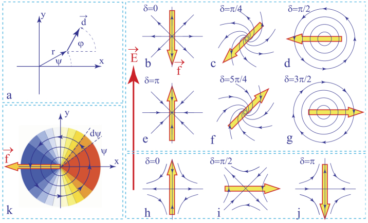
Figure 4.69. Configurations of dowsons d+ and d- and their motions in an electric field. (a) Definition of polar coordinates. (b–g) Configurations of the dowson d+. (h–j) Configurations of the dowson d-. Direction of the force f indicated in schemes b-j are given by equation [4.115], with Pfe > 0. (k) Level representation of the dielectric energy density around the dowson d+ in its circular configuration
All possible configurations of dowsons can be expressed as
with angles ψ and φ defined in Figure 4.69(a). ϕo is an angular variable and m is the topological charge equal to +1 and -1 for dowsons d+ and d-, respectively.
The interaction of dowsons with the electric field is expressed by the energy density per unit area
In a sector of the angular width dψ and length r, making the angle ψ with the x axis (see Figure 4.69(k)), the dielectric energy is thus
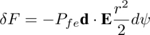
so that there is a force
acting on the dowson. Using expression [4.111], we obtain the total force
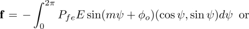
which depends on both the topological charge m and the configuration of dowsons determined by ϕo .
The directions of the force f (indicated in Figure 4.69) correspond to the case of Pfe > 0. In particular, the force f acting on the dowson d+ in its radial outward and inward configurations (see Figure 4.69(b) and (e)) is, respectively, antiparallel and parallel to the electric field.
The radial outward configuration, satisfying both the boundary condition and the action of the cuneitropism, can be reached through a spontaneous viscoelastic relaxation. This process that can last a few hours in a droplet with the radius in the range of a few millimeters, and can be made almost instantaneous by the application of a diverging Poiseuille flow accompanying the reduction of the slide/lens gap thickness (Figure 4.21 in section 4.4.1.1). By the same rheotropic mechanism, the converging Poiseuille flow, driven by an increase in the gap thickness, can force the radial inward configuration. This inward configuration is unstable so that it can return to the outward configuration by viscoelastic relaxation. Nevertheless, as the characteristic time of this relaxation process is of the order of several hours, the experiments testing the validity of equation [4.115] can be easily carried out.
The results of experiments with the outward and inward radial configurations of the dowson d+ in MBBA are depicted in Figure 4.70. The spatiotemporal cross-sections in the last column show that the directions of motion are reversed between the two radial configurations. As they are also opposite to those in Figures 4.69(b) and (e), we can conclude, in agreement with the results discussed in section 4.6.5, that the flexo-electric polarization in MBBA Pfe is antiparallel to the dowser field d. The same experiments performed with 5CB directly agree with the theoretical schemes in Figures 4.69(b) and (e), because in 5CB, Pfe is parallel to the dowser field d.
The zig-zag shaped trajectories of the dowson d+ in the spatiotemporal cross-section in Figure 4.70 also show that the direction of motion is instantaneously reversed upon the reversal of the electric field. Assuming that the velocity of motion is proportional to the driving force given in equation [4.115], this feature also agrees with theoretical predictions.
4.12. Stabilization of dowsons systems by inhomogeneous fields with defects
4.12.1. Gedanken experiment
When any complex configuration of dowsons is allowed to relax in the presence of the cuneitropic torque (due to the plane/sphere geometry of the gap) alone, the ground state of the dowser field – the radial outward configuration with one dowson d+ in the center – is always reached.
However, if the gap thickness h(x,y) had a more complex topography, such as the one represented in Figure 4.71(a), the cuneitropic torques would align the dowser field d along the thickness gradient g shown in Figure 4.71(b) and a square network of alternating dowsons d+ and d- would be stabilized by these means.
Similarly, the same network of dowsons would be stabilized by an electric field E (Figure 4.71(b)), derived from the periodic potential U(x,y) represented in Figure 4.71(a).
In such a periodic electric potential, stable positions of dowsons d+ and d- are located in extrema and saddle points, respectively.
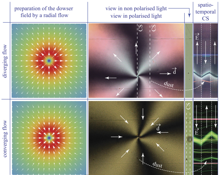
Figure 4.70. Motion of the dowsons d+ and of dust particles in electric field (MBBA)
Figure 4.71. Gadanken experiment: stabilization of a dowsons network by tropisms of the dowser texture. (a) Topography of the gap thickness h(x,y) or of the electric potential U(x,y). (b) Dowser field d oriented by the corresponding thickness gradient g = ∇h or electric field E = ∇U. (c) Simulation of the pattern of isogyres seen in polarized light
4.12.2. Triplet of dowsons stabilized in MBBA by a quadrupolar electric field
Such a periodic electric field cannot be realized by means of etched ITO electrodes. Therefore, inspired by the microfluidic study of Giomi et al. (2017), we used a much simpler system of four electrodes from Figure 4.38(c4), generating a quadrupolar electric field. The series of six pictures in Figure 4.72 shows that in the presence of such a quadrupolar electric field, the viscoelastic relaxation of a dowser field containing many dowsons leads to the stable triplet of dowsons shown in Figure 4.72(f).
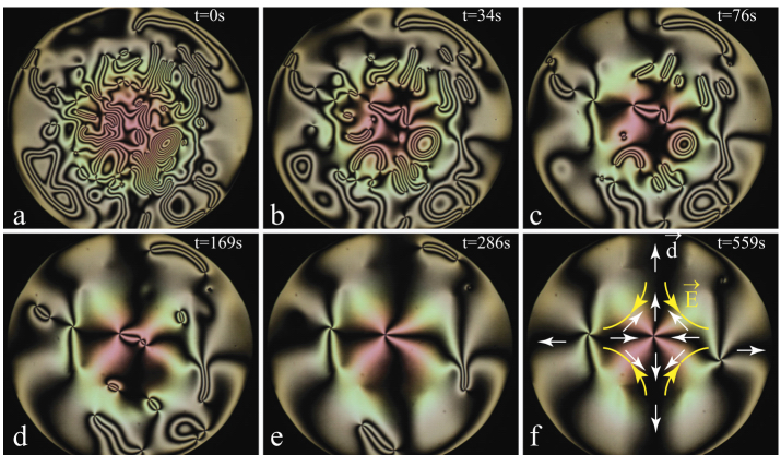
Figure 4.72. Triplet of dowsons stabilized by a quadrupolar electric field. (a) Initial configuration. (a–f) Relaxation through the annihilation of dowsons pairs. (f) Final triplet configuration stabilized by the electric field. In MBBA, the dowser field is antiparallel to the electric field
As expected, by analogy with the work of Giomi et al. (2017), the dowson d- is located in the stagnation point of the electric field (saddle point of the potential U). From the isogyres’ pattern in Figure 4.72(f), it is possible to infer that the dowser field d around this dowson d- is antiparallel to the electric field E. This is because, as we know from section 4.6, in MBBA the flexo-electric polarization P = Pfed is antiparallel to d.
4.12.3. Septet of dowsons in MBBA stabilized by a quadrupolar electric field
Figure 4.73 shows that in a stronger electric field, beside the triplet state (Figure 4.73(b)), a septet of dowsons can also be stabilized by the quadrupolar electric field (Figure 4.73(c)). It contains the same triplet of dowsons as in Figure 4.73(b) and two additional pairs of dowsons, which are located in field-free areas above the two positive ITO electrodes.
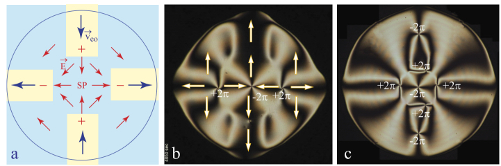
Figure 4.73. Triplet and septet of dowsons. The septet configuration is stabilized by electro-osmotic flows, which are parallel to the electric field in MBBA
In the absence of the electric field, the annihilation of these two dowsons pairs is hindered by the electro-osmotic flows shown in Figure 4.73(a). In MBBA, they have the same direction as the electric field in the adjacent gap.
4.12.4. Dowsons d+ stabilized by corner singularities of the electric field
A quadrupolar electric field with the stagnation point stabilizing the dowson d- can also be generated with the system of electrodes d6 shown in Figure 4.74(a) (see also Figure 4.38(d6)). It displays a pertinent difference with the system d4: besides the central stagnation point, it also contains four point singularities of the electric field at corners of electrodes that are susceptible to stabilize dowsons d+.
As expected, in an experiment realized with MBBA (see Figure 4.74(b)), the two dowsons d+ of the triplet configuration are located at sharp corners of negatively charged electrodes. In the same experiment realized with 5CB, the triplet of dowsons has a different orientation because the flexo-electric polarization Pfe in 5CB is parallel to the dowser field d, while in MBBA it is antiparallel to d.
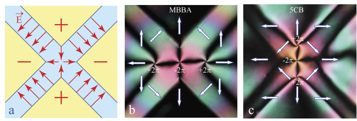
Figure 4.74. Stable configurations of a dowsons’ triplet (d+,d-,d+) in a quadrupolar electric field. (a) Electric field generated by the system of four ITO electrodes. It contains one stagnation point and four angular singularities. (b) Dowsons triplet in MBBA. The dowson d- is trapped in the stagnation point, while the two dowsons d+ are located at angular singularities of negatively charged electrodes. (c) The same experiment with a 5CB droplet. Here, the two dowsons d+ are located at angular singularities of positively charged electrodes
4.13. Dowser field submitted to boundary conditions with more complex geometries and topologies
All of the experiments discussed so far in this chapter have been performed with nematic droplets held by capillarity in the center of the lens/slide gap (see Figure 4.75(a)). In the case of 5CB, the homeotropic anchoring condition at the nematic/air interface imposes the radial outward anchoring of the dowser field at the meniscus of nematic droplets considered as solid two-dimensional simply connected discs. We emphasized several times that the ground state of the dowser field compatible with these boundary conditions is radial, directed outward, and it must contain at least one dowson d+ (see Figure 4.75(b)).
Studies of the dowser field in geometries other than the trivial one of a disc, have been initiated by the microfluidic studies of Sengupta (2013, 2015, 2018) and Giomi et al. (2017). This direction appears to be promising because in a single annular droplet, or in more complex networks of channels connected by n-junctions, the structure and topology of the dowser field d, imposed by anchoring conditions at lateral walls of channels, can be quite complex, as we will see below.
4.13.1. Ground state of the dowser field in an annular droplet
Let us first consider an annular droplet (shown in Figure 4.75(c)) with the homeotropic anchoring of the director field n at its lateral menisci (see Figure 4.75(a)). It is contained between a lens and a glass slide with a hole in its center. As we already know, the resulting preferential orientation of the field d at the two menisci is “homeotropic outward”, i.e. orthogonal to them and oriented in outward directions (see Figures 4.75(f) and (f’)).
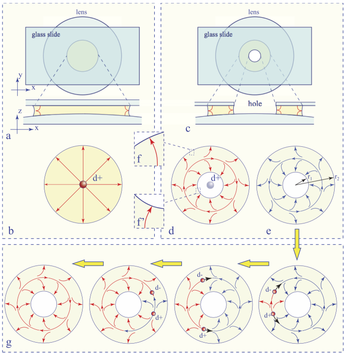
Figure 4.75. Dowser fields in a circular annular droplet. (a and b) Radial dowser field in a circular droplet with a dowson d+ in its center. (c–e) Clockwise and anticlockwise versions of the ground state of the dowser field in the annular droplet. There is a virtual dowson d+ in the hole of the annular channel. (f and f’) Homeotropic outward anchoring of the dowser field at the nematic/air menisci. (g) Transformation of the anticlockwise dowser field into the clockwise one by nucleation, motion and annihilation of a dowsons’ pair d+d-
In contradistinction to the case of the circular droplet shown in Figure 4.75(b), the dowser field imposed by these boundary conditions of the annular droplet is defect-less, though there is a virtual dowson d+ inside of the hole. In the absence of dowsons pairs, the dowser field d in such a single annular droplet is still non-trivial because it must have, on average, either a clockwise or an anticlockwise curl (see Figures 4.75(d) and (e)). Figure 4.75(g) shows that the sign of the curl can be reversed by a three-stage process: (1) generation of a dowsons pair d+d-, (2) circular motion of dowson in opposite clockwise and anticlockwise directions (see Figure 4.75(g)) and (3) annihilation of the dowsons pair.
4.13.2. Wound up metastable states of the dowser field in the annular droplet
The equilibrium states of the dowser field in the annular droplet must satisfy the requirement of vanishing the elastic torque, expressed as
as well as the radial outward boundary conditions: φ(r2,ψ) = ψ and φ(r1,ψ) = (2n +1)π + ψ at the outer and inner menisci of radii r1 and r2. The phase field φ(r) in equilibrium can be thus expressed as
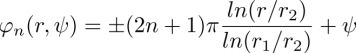
The two ground states shown in Figure 4.75(d) correspond to n = 0. Alternatively, these ground states can be seen as circular π-walls and the states with n > 0 can be seen as sets of 2n + 1 concentric π-walls.
In contradistinction with the case of the circular droplet in which 2π-walls can shrink and finally collapse (when the configuration of the central d+ dowson is free to evolve, see Figure 4.35), the radial outward anchoring condition at the inner meniscus of the annular droplet hinders the shrinking of π-walls. For this reason, the states with n > 0, such as the ones in Figure 4.76, are metastable.
The transitions between states with different n must be mediated by the three-stage process discussed above involving the generation, motion and annihilation of dowsons pairs.
4.13.3. Dowser field in a square network of channels, four-arm junctions
More complex topologies of square or triangular networks of channels are shown in Figures 4.77 and 4.78.
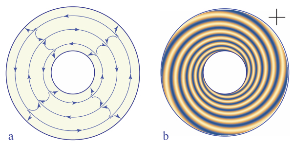
Figure 4.76. Excited metastable state of the dowser field in an annular droplet. (a) The dowser field. (b) Isogyres pattern
In the case of a square network of identical channels (with a rectangular section), in Figure 4.77 we show two versions of the dowser field compatible with the homeotropic outward anchoring at lateral walls of channels.
The first version in Figure 4.77(a) can be qualified as “microfluidic” because it is also compatible with the flow pattern indicated with large blue arrows. The directions of the dowser field are imposed by the rheotropic torques. It contains 11 dowsons dlocated at centers of cross shaped four-arm junctions of channels, as well as at certain three-arm junctions at the boundaries of the network (see section 4.13.6). There are also 12 d+ virtual dowsons located inside of the square shaped islands surrounded by channels. The total topological charge of the whole network is 12-11 = +1, as required by the homeotropic outward anchoring conditions at the external border of the network.
The second version in Figure 4.77(a) is also compatible with the boundary conditions. However, its compatibility with a flow pattern would require the presence of sources and sinks.
4.13.4. Triangular network, six-arm junctions
The dowser field in the triangular network of the channels shown in Figure 4.78 can also be qualified as microfluidic because it satisfies the anchoring conditions, as well as the orienting action of the flow pattern indicated with blue arrows. It is composed of six-arm junctions studied by Giomi et al. (2017).
The flow pattern is such that the junctions contain two stagnation points, in which the dowsons d- are located.
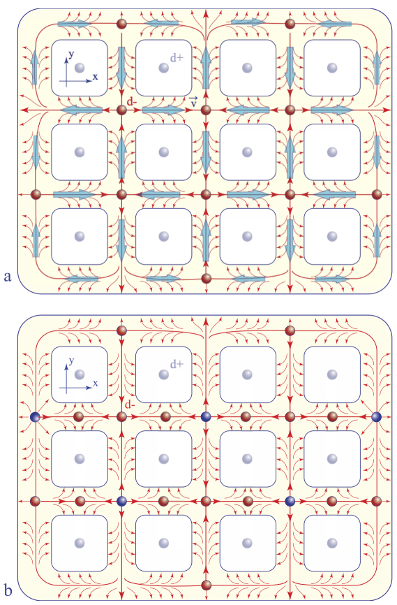
Figure 4.77. Possible dowser fields in a square network of channels. (a) Microfluidic version compatible with rheotropism, conservation of flow and boundary conditions. (b) Static version only compatible with boundary conditions

Figure 4.78. Dowser field in a triangular network of microfluidic channels. The number of six-arm junctions of channels is half that of islands. For the conservation of the total topological charge zero, there are two dowsons d- at each six-arm junction
4.13.5. Three-arm junctions
The square network of channels shown in Figure 4.77 also contain three-arm junctions at its boundaries. The three different configurations of the dowser field inside of them are listed in Figure 4.79.
4.13.6. General discussion of n-arm junctions
After detailed discussions of the dowser field inside the three-, four- and six-arm junctions, we are ready to draw general conclusions. For the sake of clarity, let us consider the example of the four-arm junction (see Figure 4.80). Its boundary is composed of eight segments.
Four of them, drawn with solid lines correspond to either lateral walls of channels treated for homeotropic anchoring, or to nematic/air interfaces imposing the same anchoring conditions of the dowser field: orthogonal and directed outward.

Figure 4.79. Dowser field in three-arm junctions. (a) Defect-less microfluidic version. (b) Microfluidic version with a dowson d- located in the stagnation point. (c) Static version with a dowson d+
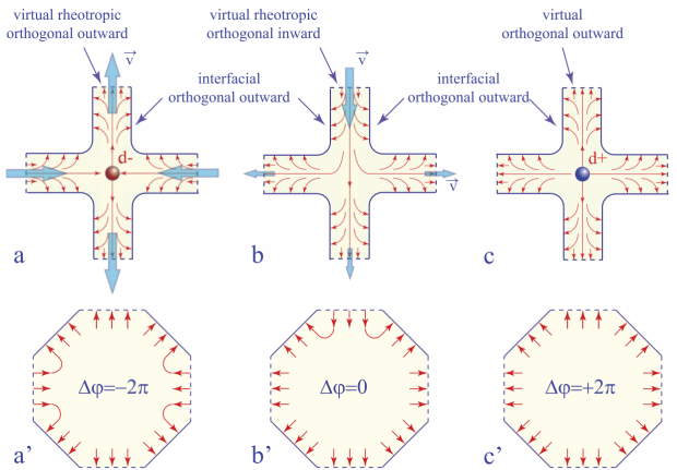
Figure 4.80. Real, and virtual anchoring conditions of the dowser field along the boundary of the four-arm junctions. (a and a’) Presence of the dowsons d- is imposed by the −2π rotation of the dowser field along the whole boundary of the junction. (b and b’) Defect-less configuration of the dowser field is a result of null rotation of the dowser field along the whole boundary of the junction. (c and c’) Presence of the dowson d+ is imposed by the orthogonal outward anchoring along the whole boundary of the junction
Four other segments drawn with dotted lines can be considered as virtual boundaries. Rheotropic torques due to Poiseuille flows across them generate virtual boundary conditions for the dowser field: orthogonal with either outward or inward directions.
The boundary of the junction in Figure 4.80(a) can be deformed continuously into the octagon shown in Figure 4.80(a’). Traveling clockwise along it results in the anticlockwise rotation of the dowser field. The topological charge of this junction is thus −2π, so that the dowser field contains at least one dowson d-.
In the second case in Figure 4.80(b), as traveling along the whole boundary (simplified to an octagon in Figure 4.80(b’)) does not produces any phase defect, the topological charge of the dowser field is thus zero.
In the last case, the topological charge resulting from boundary conditions is +2π so that the junction contains one dowson d+.
Using the same method, the boundary of any other n-arm junction can be represented as a topologically equivalent 2n-gon with n real and n virtual sides, allowing the easy determination of the topological charge. In Figure 4.81, we show examples of the three-arm and six-arm junctions discussed previously.
4.14. Flow-induced bowson-dowson transformation
Giomi et al. (2017) reported on microfluidic experiments realized with four-, sixand eight-arm junctions. Like in the experiments by Liu et al., upon the application of Poiseuille flows (see Figures 4.82(c) and (c’)), the homeotropic texture in the four-arm junction is continuously deformed by hydrodynamic torques into the bowser texture. The direction and the amplitude of the bow-like distortion is characterized by the vector b defined in Figures 4.82(c’) and 4.19(a’). In the limit of small distortions, we have
Therefore, as the Poiseuille flow in the four-arm junction contains a stagnation point, the bowser field b(x,y) contains a -2π defect, which can be called bowson b-. Let us remark that by contradistinction with the dowson d-, the bowson b- is not a true topological defect because it appears and disappears “softly” when the flow with a stagnation point is gently switched on and off.
When the flow velocity vmax is larger than vco, the flow-assisted homeotropic-dowser transition occurs and the width of the boundary dowser layers grows (see section 4.3.2). After the coalescence of the dowser boundary layers (see Figures 4.82(d) and (d’)), a small domain of the bowser texture remains in the center of the junction. Finally, it collapses and the bowson b- is replaced by the dowson d(see Figures 4.82(e) and (e’)).

Figure 4.81. Real, and virtual anchoring conditions of the dowser field along the boundary of the three- and six-arm junctions. (a–c) Dowser fields in three-arm junctions. (a’–c’) Topologically equivalent representation of boundaries. (d–f) Dowser fields in six-arm junctions. (d’–f’) Topologically equivalent representation of boundaries
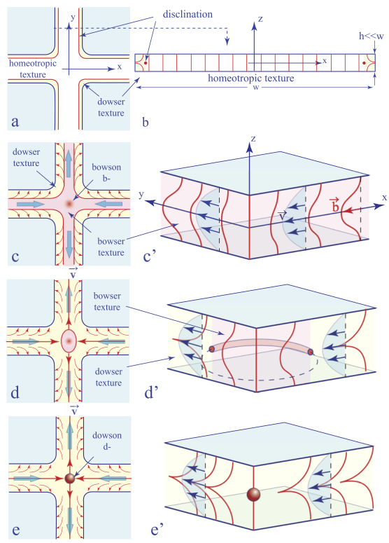
Figure 4.82. Flow-induced bowson-dowson transformation in the four-arm microfluidic junction. (a) Ground state: coexistence of the homeotropic texture with the dowser texture in boundary layers. (b) Cross-section of the channel in the ground state. (c and c’) Application of the Poiseuille flow. The homeotropic texture is continuously deformed into the bowser texture containing a -2π bowson located in the stagnation point of the flow. The width of the dowser boundary layers grows upon the flow-assisted homeotropic-dowser transition. (d and d’) Small bowser domain before its final collapse. (e and e’) The dowser texture with the dowson d- located in the stagnation point. Remark: This texture satisfies the anchoring conditions so that it is preserved after cessation of the flow
In the six-arm junctions, the ground state homeotropic texture matches the lateral walls through the dowser boundary layers. Upon application of the Poiseuille flow, the homeotropic texture is continuously deformed into the bowser one and two bowsons b- appear “softly” in stagnation points. When the flow velocity vmax is larger than the critical velocity vco (given in equation [4.16]), the flow-assisted bowser-dowser transition increases the width of the dowser boundary layer. Finally, after the coalescence of the boundary layers and the collapse of the remaining bowser domains, two dowsons d- replace the bowsons b-.

Figure 4.83. Sengupta instability of the dowson’s d- position in the four-arm junction. (a) Stable central position in slow flows. (b) For v > vcrit, the dowson d- leaves the central position and a narrow 2π-wall is created. (c) Detailed view of the 2π-wall. (d and e) Views of the instability in polarized light (courtesy of Anupam Sengupta)
4.15. Instability of the dowson’s d- position in the stagnation point
Experiments with the four-arm junctions reported in Giomi et al. (2017) have shown that the position of the dowson d- in the stagnation point of the Poiseuille flow is unstable above certain critical flow rate (see Figure 4.83). To understand the origin of this instability, we have to examine the balance of forces acting on the dowson d-when it leaves the center of junction O that coincides with the stagnation point of the flow (see Figure 4.83).
In the absence of flow, the central position of the dowson is stable because it minimizes its elastic interaction with the lateral boundaries of channels with orthogonal outward anchoring conditions. In a first approximation, the elastic restoring force is proportional to the deviation ![]() from the center O:
from the center O:

where α > 0 is a numeric factor.
In the presence of a flow with a stagnation point SP located in the center O, the convection of the distortion (discussed in section 4.7.3) generates a viscous force, which can be written as

where β > 0 is another numeric factor.
The total force acting on the dowson d- is thus
with

For vmax > 0 (see Figure 4.83(b)), the coefficient Cx is negative so that the central position of the dowson d- is stable with respect to deviations δx along the x axis. Stability with respect to deviations δy depends on the sign of the second coefficient Cy. For flow velocities larger than the critical value given by

Cx is positive so that an instability occurs: the dowson d- leaves the center of the junction and moves along the y axis. Let us emphasize that due to its rheotropism, the dowser field d still remains aligned by the flow, except for a 2π-wall, which now connects the dowson to the stagnation point SP (see Figures 4.83(b) and (d)).
4.16. Appendix 1: equation of motion of the dowser field
In nematodynamics, the equation of motion of the director field is derived from the balance of the elastic, viscous, magnetic or electric torques (per unit volume) acting on the director field n(x,y,z,t):
From the discussion of the dowser texture given in section 4.1.3.1, we know that the director field expressed as
with
has, in principle, only one degree of freedom: the azimuthal angle φ(x, y, t). Therefore, only the z components of the torques listed in equation [4.125] are involved in the motions of the dowser field. Moreover, the dependence of all of the components Γz on the z coordinate is set by the expression θ = πz/h.
For these two reasons, it is convenient to consider the dowser texture as a two dimensional system and rewrite equation [4.125] as a balance of torques per unit area acting on the dowser field.
4.16.1. Elastic torque
4.16.1.1. Uniform thickness h
In the approximation of the isotropic elasticity with K1 = K2 = K3 = −K4 = K and assuming that K13 = 0, the elastic torque per unit volume acting on the director field takes a simple form (see sections B.II.2 and B.II.3 in Oswald and Pieranski (2005))
With equation [4.126], its z component writes
After integration on z, we obtain the elastic torque per unit area:
To end this discussion, let us remark that the last K13 term of the elastic energy density
does not contribute to elastic torques in bulk. Its action on surfaces with strong anchoring conditions is negligible.
4.16.1.2. Cuneitropic torque in a thickness gradient
In Pieranski et al. (2016a) and in section 4.5.3, we have shown that in samples without uniform thickness h, there is an additional elastic torque proportional to the thickness gradient ![]() :
:

4.16.2. Viscous torques
In nematodynamics, the viscous torque acting on the director n can be expressed as
In the first term of this expression, N, defined as
represents the relative angular velocity of the director n with respect to the surrounding fluid of vorticity
In the second term of the equation [4.133], the tensor
corresponds to the symmetric part of the velocity gradients tensor.
In the absence of flows, the z component of the viscous torque [4.133] integrated on z has already been calculated in section 4.4.6.2:
A Poiseuille flow
generates an additional torque per unit volume

Using equations [4.135] and [4.136], and after integration on z, we obtain three other contributions to the viscous torque per unit area.
The first one
is identical to expression [4.24] of the rheotropic torque calculated in Pieranski et al. (2017) and already discussed in section 4.4.1.2, because γ2 − γ1 = 2α2. This contribution is related to the gradient of the velocity v with respect to z.
The second contribution

The last contribution
can also play a role in the vicinity of boundaries, as well as in stagnation points of microfluidic flows.
4.16.3. Magnetic torque
The magnetic torque acting on the dowser field discussed and calculated in section 4.5.1, is given by
where χa = χ// − χ⊥ is the anisotropy of the magnetic susceptibility.
4.16.4. Electric torque
The electric torque acting on the dowser field was discussed and calculated in Pieranski and Godinho (2019b) and in section 4.6.1. It is given by
where ![]() is the anisotropy of the dielectric permittivity and Pfe is the flexo-electric polarization.
is the anisotropy of the dielectric permittivity and Pfe is the flexo-electric polarization.
4.17. References
Blinov, L. and Chigrinov, V. (1996). Electrooptic Effects in Liquid Crystal Materials. Springer-Verlag, New York.
Boyd, G., Cheng, J., Ngo, P. (1980). Liquid-crystal orientational bistability and nematic storage effects. Appl. Phys. Lett., 36, 556–558.
Cabeça, R., Godinho, M., Pieranski, P. (2019). Magnetic tweezers for captive disclination loops. The European Physical Journal Special Topics, 227(17), 2439–2454.
Cladis, P. and Brand, H. (2003). Hedgehog-antihedgehog pair annihilation to a static soliton. Physica A, 326, 322–332.
Cladis, P., Saarloos, W., Finn, P., Kortan, P. (1987). Dynamics of line defects in nematic liquid crystals. Phys. Rev. Lett., 58, 222–225.
Cladis, P., Finn, P., Brand, H. (1995). Stable coexistence of spiral and target patterns in freely suspended films of smectic-c liquid crystals. Phys. Rev. Lett., 75, 2945.
Čopar, S., Seč, D., Aguirre, L., Almeida, P., Dazza, M., Ravnik, M., Godinho, M., Pieranski, P., Žumer, S. (2016). Sensing and tuning microfiber chirality with nematic chirogyral effect. Physical Review E, 93(3), 032703.
Dozov, I., Martinot-Lagarde, P., Durand, G. (1982). Flexoelecrically controlled twist of texture
in a nematic liquid crystal. J. Phys. Lett., 365, 356–369.
Embon, L., Anahory, Y., Jelić, V., Lachman, E., Myasoedov, Y., Huber, M., Mikitik, G., Silhanek, A., Milošević, M., Gurevich, A., Zeldov, E. (2017). Imaging of super-fast dynamics and flow instabilities of superconducting vortices. Nature Communications, 8, 85.
Emeršič, T., Zhang, R., Kos, Z., Čopar, S., de Pablo, J., Tkalec, U. (2019). Sculpting stable structures in pure liquids. Sci. Adv., 5, eaav4283.
Fazzio, S., Nannelli, F., Komitov, L. (2001). Sensitive methods for estimating the anchoring strength of nematic liquid crystals on Longmuir-Blodgett monolayers of fatty acids. Phys. Rev. E, 63, 061712.
Friedel, G. (1922). Etats mésomorphes de la matière. Annales de physique, 18, 273.
de Gennes, P.-G. (1972). Types de singularités permises dans une phase ordonnée. CRAS, 275, 319–321.
de Gennes, P.-G. and Prost, J. (1993). The Physics of Liquid Crystals. Clarendon Press, Oxford.
Gilli, J., Thiberge, S., Vierheilig, A., Fried, F. (1997). Inversion walls in homeotropic and cholesteric layers. Liq. Cryst., 23, 619.
Giomi, L., Kos, Ž., Ravnik, M., Sengupta, A. (2017). Cross-talk between topological defects in different fields revealed by nematic microfluidics. Proceedings of the National Academy of Sciences, 114(29), E5771–E5777.
Hadjiefstatiou, E. and Montagnat, L.-M. (2017). La course des monopôles nématiques, L2 Internship. Laboratoire de Physique des Solides, Université Paris-Saclay, Orsay.
Hindmarsh, M. (1995). Where are the hedgehogs in quenched nematics? Phys. Rev. Lett., 75, 2502.
Kleman, M. and Lavrentovich, O. (2006). Topological point defects in nematic liquid crystals. Phil. Mag., 86, 4117–4137.
Kurik, M. and Lavrentovich, O. (1988). Defects in liquid crystals: Homotopy theory and experimental studies. Sov. Phys. Usp., 31, 196–223.
Lavrentovich, O. (1992). Geometrical anchoring at an inclined surface of a liquid crystal. Phys. Rev. A, 46, R722.
Lavrentovich, O. and Rozhkov, S. (1988). Strings with boojums at their ends: Topological defects of a new type in nematic liquid crystals. JETP Lett., 47(4), 254–258.
Link, D., Nakata, M., Takanishi, Y., Ishikawa, K., Takezoe, H. (2001). Flexo-electric polarisation in hybrid nematic films. Phys. Rev. E, 65, 019701(R).
Liu, Z., Luo, D., Yang, K.-L. (2019). Flow-driven disclination lines of nematic liquid crystals inside a rectangular microchannel. Soft Matter, 15(28), 5638–5643.
Meyer, R. (1969). Piezoelectric effects in liquid crystal. Phys. Rev. Lett., 22, 918–921.
Meyer, R. (1972). On the existence of even indexed disclinations in nematic liquid crystals. Phil. Mag., 27, 405–424.
Musěvič, I., Škarabot, M., Tkalec, U., Ravnik, M., Žumer, S. (2006). Two-dimensional nematic colloidal crystals self-assembled by topological defects. Science, 313, 954–957.
Nabarro, F. (1972). Singular lines and singular points of ferromagnetic spin systems and of nematic liquid crystals. J. de physique, 33, 1089–1098.
Oswald, P. and Pieranski, P. (2005). Nematic and Cholesteric Liquid Crystals, Concepts and Physical Properties Illustrated by Experiments. CRC Press, Taylor and Francis, London, New York, Singapore.
Oswald, P., Poy, G., Vittoz, F., Popa-Nita, V. (2013). Experimental relationship between surface and bulk rotational viscosities in nematic liquid crystals. Liqu. Cryst., 40, 734–744.
Pieranski, P. (2019). Pierre-Gilles de Gennes: Beautiful and mysterious liquid crystals. Comptes rendus physique, 20, 756–769.
Pieranski, P. and Godinho, M. (2019a). Electro-osmosis and flexo-electricity in the dowser texture. EPJE, 42, 69.
Pieranski, P. and Godinho, M. (2019b). Flexo-electricity of the dowser texture. Soft Matter, 15, 1469–1480.
Pieranski, P. and Godinho, M. (2020). On generation, motions and collisions of dowsons. Frontiers in Physics 7, Article 238.
Pieranski, P., Godinho, M. and Čopar, S. (2016a). Persistent quasiplanar nematic texture: Its properties and topological defects. Phys. Rev. E, 94, 042706.
Pieranski, P., Čopar, S., Godinho, M., Dazza, M. (2016b). Hedgehogs in the dowser state. EPJE, 39, 121.
Pieranski, P., Hulin, J.-P., Godinho, M. (2017). Rheotropism of the dowser texture. EPJE, 40, 109.
Poincaré, H. (1886). Sur les courbes définies par les équations différentielles. J. de math., 2(4), 151.
Poulin, P., Stark, H., Lubensky, T., Weitz, D. (1997). Novel colloidal interactions in anisotropic liquids. Science, 275, 1770–1773.
Sengupta, A. (2015). Topological microfluidics: Present and prospects. Liquid Crystals Today, 24(3), 70–80.
Sengupta, A. (2018). Nematic liquid crystals and nematic colloids in microfluidic environment, PhD Thesis. Georg-August-Universität, Göttingen.
Sengupta, A., Tkalec, U., Ravnik, M., Yeomans, J., Bahr, C., Herminghaus, S. (2013). Liquid crystal microfluidics for tunable flow shaping. Physical Review Letters, 110(4), 048303.
Srinivasan, G. (2020). Disinclinaisons et parois dans les cellules nématiques torsadées, M1 Internship. Laboratoire de Physique des Solides, Université Paris-Saclay, Orsay.
Tang, X. and Selinger, J. (2020). Minimisation principle for shear alignement of liquid crystals. Phys. Rev. E, 101, 032701.
Ternet, D., Larson, R., Leal, L. (1999). Flow-aligning and tumbling in small-molecule liquid crystals: Pure components and mixtures. Rheologica Acta, 38(3), 183–197.
Wang, M., Li, Y., Yokoyama, H. (2017). Artificial web of disclination lines in nematic liquid crystals. Nature Communications, 8(1), 1–7.
Williams, C., Pieranski, P., Kleman, M. (1972). Nonsingular s=+1 screw disclination lines in nematics. Phys. Rev. Lett., 29, 90–92.