
Mathematics and Statistics Tutorial
Pascal Wallisch
Not everyone who intends to start practicing the neurosciences can be expected to do so with a perfect knowledge of mathematics. As a matter of fact, due to the inherently interdisciplinary nature of the field, it would be quite surprising if this were the case. Educational backgrounds are diverse, and not everyone is privileged enough to hail from a “math-heavy” one as afforded by physics, computer science, or engineering. Thus, the purpose of this tutorial is largely therapeutic in nature. We will focus on introducing a few key concepts in linear algebra and statistics that are central to neuroscience research. We will do so in the most gentle and affirming way possible. In the process, the reader will (hopefully) realize how MATLAB® itself can be used to help overcome math anxiety.
Keywords
mean; variance; Student’s t distribution; linear algebra; matrices; vectors; arrays; Bayesian distribution; probability
3.1 Introduction
Not everyone who intends to start practicing the neurosciences can be expected to do so with a perfect knowledge of mathematics. As a matter of fact, due to the inherently interdisciplinary nature of the field, it would be quite surprising if this were the case. Educational backgrounds are diverse, and not everyone is privileged enough to hail from a “math-heavy” one as afforded by physics, computer science, or engineering (to be sure, plenty do, but they tend to be similarly challenged by a lack of prior exposure to biological concepts). This state of affairs can usually be traced to the quality and style of the typical high school and college education in mathematics, which tends to be heavy on proofs and rote memorization of formulae, but falls short on good explanations that could foster conceptual understanding, visualization, and establishing a working knowledge that allows problem solving. In reality, the only thingk most people actually learn (in terms of long term retention) from their high school education in mathematics is that the field is deeply foreign and full of alien and intimidating topics that can trigger deep-seated insecurities. But people do learn, so most usually stay clear of math-heavy fields after an initial negative exposure if they can help it, further solidifying the deficiency. Worse than just the absence of knowledge, many people are actively avoiding math. In our information-based society, few admissions of ignorance are received with such impunity and, indeed, acclaim as that of “not getting math.” Math phobia has swept wide parts of the population and is flaunted as a badge of honor. The biological sciences are not immune from this; citations of a paper drop 35% for every additional equation per page (Fawcett et al., 2009). Yet a solid and workable knowledge of some key mathematical concepts is absolutely indispensable if one is to follow and partake in contemporary neuroscience research. There is no question that not overcoming the acquired fear of math will be severely limiting if not debilitating to the budding researcher, a state of affairs that will only get more severe as the mathematization of neuroscience progresses relentlessly. Such self-limitation is needless, and it is a shame that droves of budding researchers trying to uncover answers to questions they care about passionately find themselves in this situation without any fault of their own.
Thus, the purpose of this tutorial is largely therapeutic in nature. We will focus on introducing a few key concepts in linear algebra and statistics that are central to neuroscience research. We will do so in the most gentle and affirming way possible. In the process, the reader will (hopefully) realize how MATLAB® itself can be used to help overcome math anxiety. One piece of advice upfront: If you know that looking at an equation raises your blood pressure, there is a straightforward trick to calm the nerves. Simply translate the equation into a series of MATLAB commands. Every equation ultimately corresponds to a couple of lines of code. Once you get familiar with MATLAB, even the most intimidating looking equation will lose its sting.
In addition to this primary goal, we will also set up the mathematical groundwork for the math that is used in the rest of the chapters, so that there are no bad surprises later on.
If you feel already sufficiently steeled in the art and practice of mathematics, you can safely skip this tutorial. If you are on the fence, you probably need the reminder (in spite of the central importance of explanations, math is effectively a motor skill; it benefits tremendously from practice).
We explicitly focus on a gentle introduction here, as it serves our purposes. If you are in need of a more rigorous or comprehensive treatment, we refer you to Mathematics for Neuroscientists by Gabbiani and Cox. If you want to see what math education could be like, centered on great explanations that build intuition, we recommend Math, Better Explained by Kalid Azad.
3.2 Linear Algebra
Linear algebra is as fitting a topic as any with which to start this tutorial. As it so happens, the central concept of linear algebra, the matrix, is also the principal data structure underlying MATLAB itself. MATLAB is at its best when it comes to the manipulation of matrices. Linear algebra is, broadly speaking, the study of matrix manipulations.
But what is a matrix and why is it so central? Didn’t we get in enough trouble when we started to mix the alphabet into equations back in middle school? What does the concept buy us? Why is it a suitable representation, and of what exactly?
We will discuss these issues in turn.
3.2.1 Matrices, Vectors, and Arrays
To avoid confusion, we need to clarify some concepts and the terms we use to reference these concepts. In linear algebra, the term scalar refers to a nondimensional quantity, whereas values commonly refers to vectors, matrices, or arrays. Informally, the terms matrix, vector, and array are sometimes used interchangeably, but more formally, an array is a set of numbers organized by a finite number of fixed sized dimensions. Within MATLAB, the term array can also denote a data structure, a set of numeric values. However, in this tutorial, we will use “array” in its mathematical sense.
A matrix is a two-dimensional array of numbers or variables. Matrices are usually depicted as a rectangular group of numbers, with rows and columns corresponding to the two dimensions. If there are more than two dimensions, we would call it a “tensor,” but let’s not get into that at this point. The sizes of the two dimensions of a matrix are often written as m×n, where m indicates the number of rows and n indicates the number of columns. Here is an example of a 2×3 matrix, A:
![]()
In MATLAB, we use square brackets for defining a matrix. The following MATLAB code defines a matrix A with the above values. The matrix name is usually capitalized.
The entire content of the matrix is contained by the square brackets, and a semicolon is used to separate the rows.
In contrast to a matrix, a vector is a one-dimensional array of numbers or variables. An individual row or column of a matrix can be identified as a row vector or a column vector. Here is an example row vector B from matrix A, above:
![]()
Just like matrices, vectors are also entered into MATLAB with square brackets.
Note that no semicolons appeared within the square brackets for the definition of B. This was because B has only a single row.
You can refer to a particular element in a matrix by its row and column placement. So, for the matrix A, the element in the first row and third column is the number 8. These two values identifying an element within the matrix are called indices. Likewise, an element of a vector can be identified with a single index.
In MATLAB, indices can be specified using parentheses to select elements from matrices or vectors. For example,
A vector would need only one index.
Some matrices are special and can be categorized further. We will refer to these definitions in the following sections.
Square matrices are those matrices where both dimensions are equal. Square matrices in which only the values along the main diagonal are non-zero are called diagonal matrices. Here is an example:

Finally, diagonal matrices where all the non-zero values are 1 are termed identity matrices. The capital letter I is usually reserved in linear algebra for representing identity matrices. Here is an example of a 4×4 identity matrix:
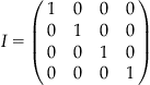
Often in linear algebra, an identity matrix is referred to as “the identity matrix,” with dimension inferred from context, and subsequent sections will adhere to this convention. MATLAB has a special function for creating an identity matrix of any desired size: eye(n), where n is the dimension desired.
There is a reason MATLAB has its own function for the identity matrix. It plays a central role in linear algebra, as will become clear in the rest of this tutorial.
3.2.2 Transposition
One common operation on matrices is transposition. Transposition flips rows and columns; each row of the original matrix becomes the corresponding column of the new matrix. In mathematical notation, transposition is usually indicated with the superscript t. Here is how we would write the transposition of the matrix A defined in the previous section.

You carry out this operation in MATLAB by using the punctuation ’ after the matrix name: In this case, A’.
These preliminaries might seem excessive, but a precise nomenclature of operations matters a lot in linear algebra. It will soon become obvious why.
3.2.3 Addition
Addition is an operation that is defined for two matrices or two vectors of the same dimensionality. Adding matrices algebraically is adding corresponding components to form a new matrix. Thus, each of the two matrices or two vectors being added must contain only elements that correspond with those in the other. Because addition is defined only for cases where the two values being added have the same dimensionality, cases where the dimensionality differ, such as adding A from the previous section with its transpose, would be termed undefined or meaningless. But you don’t actually have to worry about this. MATLAB will literally not let you add matrices with differing dimensionalities; it will complain that there has been an error and that “Matrix dimensions must agree,” all red and bothered (unless you changed the color preferences).
Here is an example of matrix addition. We define the matrix F as
![]()
![]()
3.2.4 Scalar Multiplication
If this is starting to look to you like we are retracing our steps from elementary school, you would be right. All operations you learned in first grade for actual numbers have their corresponding operation for arrays in linear algebra (except for transpose; that wouldn’t make any sense for scalars, as each scalar is its own transpose, so we mercifully skipped that in elementary school; now you know). Note that if you add A to itself, as in Exercise 3.1, the resulting matrix has values double to those of the corresponding values in A. This suggests a simple definition for the scalar multiplication of a matrix. Indeed, when a matrix is multiplied by a scalar value, each element of the matrix is simply multiplied by that number.
![]()
In MATLAB, a scalar multiplication is performed with an asterisk, if one of the multiplicants is a scalar number.
3.2.5 Matrix Multiplication
So far, so simple. But this is the precise point where things get hairy and the majority of students get lost with linear algebra. This is because matrix multiplication is the first point where the analogy to elementary school math starts to break down. As you already learned elementary school math, this highly practiced cognitive template will start to interfere with learning this crucial step. We urge you to pay extreme attention to matrix multiplication and practice it as much as you can to override your strong cognitive priors. As most of linear algebra crucially hinges on matrix multiplication, this dire warning is not overstated. This is the point where you most likely will get lost, if you get lost. So proceed with the utmost care.
Multiplication can also be defined for two matrices or for two vectors. When you multiply two matrices together, AB, each element of the resulting matrix, C, is the sum of the corresponding row elements of A times the corresponding column elements of B. In other words, all elements of C may be obtained by using the following simple but perhaps counterintuitive rule (we are not big fans of rote memorization, but it pays to memorize this one by heart; otherwise, it will haunt you forever):
The element in row i and column j of the product matrix AB is equal to the row i of A times the column j of B, added.
Here is an example with two square matrices C and D.
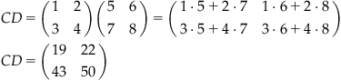
This definition constrains the dimensionality of the two matrices or vectors in a matrix multiplication. For two matrices A and B, the number of columns in A must match the number of rows in B for the product AB to be defined. Also, the dimensions of the product are m×n, where m is the number of rows in A and n is the number of columns in B. If you try to multiply “incompatible” matrices (in terms of dimensionality), MATLAB won’t let you do it and will inform you of this fact.
Matrix multiplication can occur between a vector and a matrix, provided that both meet the dimensionality constraints.
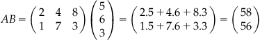
Observe that AB is not the same as BA, throwing off elementary school intuitions. Unlike scalar multiplication, matrix multiplication is not commutative; in general, matrices do not commute under multiplication. In the mathematical sense, commuting has nothing to do with traveling to your place of business. It simply means, as stated above, that AB is not the same as BA. It is extremely important to keep this property in mind when manipulating non-scalar values in algebraic equations.
In MATLAB, matrix multiplication also uses the asterisk like scalar multiplication, but both multiplicants are now non-scalars:
Much like in non-matrix multiplication where every number N has a reciprocal such that ![]() , matrix multiplication defines the concept of an inverse. However, unlike with scalar multiplication, only some matrices have inverses. We were not kidding when we mentioned that matrix multiplication is where the vanilla world of elementary school scalar multiplication is shattered.
, matrix multiplication defines the concept of an inverse. However, unlike with scalar multiplication, only some matrices have inverses. We were not kidding when we mentioned that matrix multiplication is where the vanilla world of elementary school scalar multiplication is shattered.
The inverse of a matrix D, D−1, is the matrix that, when multiplied with the original matrix, equals the identity matrix:
![]()
Note that this definition requires that the matrix D be square. This falls out from the constraints of matrix multiplication and the definition of the identity matrix as a square matrix.
So, for example, if we define D as
![]()
![]()
For your convenience, MATLAB provides a function inv(A), which calculates the inverse of a matrix.
As mentioned above, only square matrices have a defined inverse. Even among square matrices, not all have inverses. The MATLAB function inv() returns Inf in such cases. For instance, the matrix X below looks completely innocent, but alas, it does not have an inverse.
As MATLAB’s warning implies, such square matrices without inverses are termed singular. We will discuss criteria for assessing when a matrix has a defined inverse when we discuss determinants, in Section 3.2.6.
3.2.6 Geometrical Interpretation of Matrix Multiplication
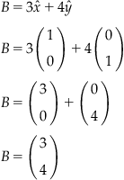
In addition to linear algebra, there is also a corresponding geometrical interpretation of matrix-vector multiplication that can be extremely useful. First, see what happens when a vector is multiplied by a scalar. Suppose that
![]()
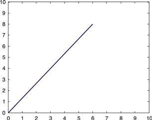
You can plot the vector B on the Cartesian plane if you assume that the x-component of the vector is the element in the first row and the y-component of the vector is the element in the second row. In such cases, we can define unit vectors ![]() and
and ![]() . Therefore, the vector B can be written in terms of simple and elementary unit-length component vectors as
. Therefore, the vector B can be written in terms of simple and elementary unit-length component vectors as ![]() . This can be readily seen by substituting the definitions for
. This can be readily seen by substituting the definitions for ![]() and
and ![]() into the equation for B:
into the equation for B:
This decomposition in terms can be demonstrated in MATLAB as well.
This results in the graph shown in Figure 3.1.

Next, you can multiply the vector B by a scalar, 2, to get:
If you plot this new vector alongside B, then you get the graph shown in Figure 3.2.
Notice that multiplying a vector by a scalar changes only its length. It does not change the direction of the vector. Now see what happens when a vector is multiplied by a matrix.
![]()
Since the matrix A is square, the product of A and B has the same dimensions as the vector B (in this case, both are 2×1). Therefore, you can plot the vectors A * B and B on the same graph to obtain the result shown in Figure 3.3.

Figure 3.3 Multiplying the vector B (blue) by the matrix produces the rotated and rescaled vector in red.
Here, you can see that multiplication of vector B by the matrix A has resulted in rotating B counterclockwise and stretching it out. Now, try another example, where A is the same, but:
![]()
If you plot B and AB on the same graph, then you get the result shown in Figure 3.4.
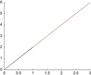
Figure 3.4 Multiplying the matrix A by the vector B=(1 2) (in blue) produces a vector with the same direction but different magnitude (in red).
In this case, multiplication of the vector B by the matrix A is equivalent to multiplication of B by a scalar—in this case 3. It turns out that this scenario is a general one. For many square matrices A, there exist corresponding vectors B such that
![]()
where ![]() is a scalar constant. (So, in the previous example,
is a scalar constant. (So, in the previous example, ![]() .)
.)
Geometrically, this means that for a given matrix A, there is a vector B that does not rotate when multiplied by A. The scalar ![]() is called an eigenvalue of the matrix A. The invariant vector B is called an eigenvector of the matrix A, and each eigenvector B is associated with a particular eigenvalue
is called an eigenvalue of the matrix A. The invariant vector B is called an eigenvector of the matrix A, and each eigenvector B is associated with a particular eigenvalue ![]() .
.
While we mentioned this concept in passing, it pays to do a full stop and truly appreciate the concept. It is even more fundamental to linear algebra than matrix multiplication itself. There are quite a few people who spend their days calculating eigenvalues of systems (represented by matrices). Even worse, there are plenty of intellectual posers who fail this basic academic shibboleth; they tellingly refer to them as “Igon values” instead (Gladwell, 2009). You don’t want to be that guy. Seriously, throwing buzzwords around is all fun and games, but we want you to actually understand them. Only if you understand these concepts can you meaningfully work with them, and we assure you that you will be dealing with eigenvalues and eigenvectors as long as you do linear algebra. And you will probably be doing linear algebra as long as you are doing science. As for how long you want to do science, that’s up to you.
Back to eigenvectors, there is actually a relatively simple visual interpretation. Imagine rotating a globe around its axis (or imagine the actual planet earth spinning around its axis on a daily basis). The values on this axis are rotation invariant: They do not change when the system is rotated. You can imagine that these are special values and it is important to know them, as they characterize in a way what the system as a whole (the spinning earth) is doing. If the system was doing something else, the values would be different.
We do believe that in addition to this visual you get the best appreciation for eigenvectors and eigenvalues not by reading or writing about them, but by working with them, which is exactly what we will do in the next few sections, where we will discuss how to determine eigenvectors/eigenvalue pairs for square matrices and their applications. However, before we can cover eigenvectors and eigenvalues, we need to discuss the determinants of matrices.
3.2.7 The Determinant
As discussed earlier, only some square matrices actually have defined inverses. The determinant is a value (defined only for square matrices) that aids in determining whether a matrix has a defined inverse or not. In addition, the determinant aids in identifying whether a matrix has eigenvectors as well.
The definition of the determinant for larger matrices is complex, and, for completeness, we refer the reader to a suitable reference. For 2×2 matrices, however, the determinant is a relatively simple expression. Defining the matrix A as
![]()
the determinant is defined as ad−bc, multiplying then subtracting the values on the two diagonals of the matrix. The determinant is written in linear algebra as det() around a matrix or as vertical bars. The following equation shows the two notations and the value of the determinant for 2×2 square matrices.
![]()
MATLAB provides a function det() that calculates the determinant of a matrix for you.
Exercise 3.7
Use MATLAB to calculate the determinant of the matrix ![]() .
.
Now you know how to calculate it. But why would you want to? The value of the determinant can be used to determine (hence the name: It actually determines a range of other matrix properties as well) whether a square matrix has a defined inverse. A square matrix has a defined inverse if and only if the determinant of that matrix is nonzero (As we saw earlier that such matrices with zero valued determinants and no inverse are called singular.) This can be seen by attempting to determine the value of a matrix inverse analytically.
Let the matrices A and A−1 be defined as
![]()
For A−1 to be the inverse of A, AA−1 must equal the identity matrix. This generates a set of equations in the elements of both matrices:
Ideally, we would want to represent the elements of A−1 in terms of a,b,c,d; the elements of A. Starting with ce+gd=0, the value of e is

Substituting this value for e into the equation ![]() results in an equation using only one term from A−1, g:
results in an equation using only one term from A−1, g:
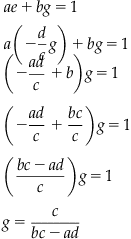
This yields an expression for the element g of A−1 solely in terms of elements of the original matrix A, and this process can be repeated for the other three elements of A−1. However, in rearranging terms, the equation was divided by the term ![]() , implying that this term must not be zero (as no one can divide by zero). You may recognize this term as the negative of the 2×2 determinant defined above, bc−ad. Thus, if the determinant is zero, the system of equations identified by the inverse has no solution. QED.
, implying that this term must not be zero (as no one can divide by zero). You may recognize this term as the negative of the 2×2 determinant defined above, bc−ad. Thus, if the determinant is zero, the system of equations identified by the inverse has no solution. QED.
3.2.8 Eigenvalues and Eigenvectors
Recall that finding the eigenvalues and corresponding eigenvectors of a square matrix A is equivalent to solving for scalar ![]() and vector B such that
and vector B such that
![]()
One valid but obviously degenerate solution to this equation is the zero vector,
![]()
regardless of the matrix A, as long as A is a 2×2 matrix. The zero-vector solution is called the trivial solution and will not be of interest here (it is rather of interest to philosophical discussions of mathematical conceptualizations of death). Thus, to limit solutions to the non-trivial solutions, we will require that any solutions for B not be zero vectors.
The eigenvector equation is ![]() , where I is the identity matrix. This can be rearranged as:
, where I is the identity matrix. This can be rearranged as:

If the matrix ![]() has an inverse, then multiplying through this equation by the inverse gives:
has an inverse, then multiplying through this equation by the inverse gives:
![]()
Because a matrix multiplied by its inverse is the identity, this would imply that
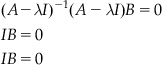
which is exactly the trivial solution that you do NOT want, which means that ![]() must not have an inverse if nontrivial solutions for B exist. Recall from the previous section that a matrix has no inverse if its determinant equals zero. So, for
must not have an inverse if nontrivial solutions for B exist. Recall from the previous section that a matrix has no inverse if its determinant equals zero. So, for ![]() , nontrivial solutions for B exist only if
, nontrivial solutions for B exist only if ![]() . QED, yet again. This equation is called the characteristic equation of the matrix A. It is the only equation you need to calculate the eigenvalues and eigenvectors of a matrix.
. QED, yet again. This equation is called the characteristic equation of the matrix A. It is the only equation you need to calculate the eigenvalues and eigenvectors of a matrix.
Through the characteristic equation, we can solve for the eigenvalues of A, ![]() , and then we can use the values of
, and then we can use the values of ![]() to determine the corresponding eigenvectors of A.
to determine the corresponding eigenvectors of A.
We use this now in an example calculation of eigenvectors and eigenvalues for the matrix
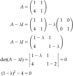
You can solve the quadratic equation for ![]() to get
to get ![]() . These are the eigenvalues of the matrix A! You can solve for the corresponding eigenvectors as follows. For
. These are the eigenvalues of the matrix A! You can solve for the corresponding eigenvectors as follows. For ![]() , the equation becomes
, the equation becomes
![]()
Substitute A into the preceding equation and let:
![]()
The preceding equation becomes:
![]()
Solving the system of equations gives y=2x. Thus, any B such that
![]()
is an eigenvector of the matrix A corresponding to the eigenvalue ![]() . Note that this demonstrates that any vector with the same orientation will be invariant to changes in orientation imposed by multiplication by A (recall the spinning globe).
. Note that this demonstrates that any vector with the same orientation will be invariant to changes in orientation imposed by multiplication by A (recall the spinning globe).
Exercise 3.8
Find the eigenvector of A corresponding to the other eigenvalue, ![]() .
.
In MATLAB, the command [V,D]=eig(A) will return two matrices: D and V. The elements of the diagonal matrix D are the eigenvalues of the square matrix A. The columns of the matrix V are the corresponding eigenvectors.
3.2.9 Applications of Eigenvectors: Eigendecomposition
Here we will describe a powerful theorem called the eigendecomposition theorem. This theorem states:
For any n×n matrix A with distinct eigenvalues you can write:
![]()
where V is the square matrix whose columns are the eigenvectors of A, and D is the square diagonal matrix formed by placing the eigenvalues of A along the primary diagonal of D.
Powerful stuff indeed. Note that the matrices V and D are exactly those matrices returned by the MATLAB function eig()!
This theorem allows any matrix A with distinct eigenvalues to be decomposed into a diagonal matrix. This decomposition is especially useful in cases where a matrix needs to be raised to a power:

Note here that each pair VV−1 between diagonal matrices D is equivalent to the identity matrix and thus drops out of the equation.
![]()
Only the diagonal matrix D is raised to the power N. Recall that a diagonal matrix raised to a power N is exceptionally easily calculated (raise each element of the diagonal to the power N). Thus, raising a matrix with distinct eigenvalues to a large power becomes a far simpler calculation.
3.2.10 Applications of Eigenvectors: PCA
The eigendecomposition theorem can be used in many remarkable ways. In this section, we will explore one application, principal component analysis (which we will revisit with practical examples in Chapter 17 of this book). Principal component analysis provides a means of identifying the independent axes responsible for major sources of variability in a multivariate sample. Once these axes are identified, the axes can be used for classification and simplification of the data. For instance, if two dimensions capture all the variability inherent in 200 dimensions, the data can be simplified to the “loading” of the data on those two dimensions. This will become clearer later on.
Let X be a set of data represented as an m×n matrix X, where m is the number of data points and n is the number of dimensions in the data set. For this data, we can calculate an n×n covariance matrix ![]() . According to the eigendecomposition theorem, we can represent
. According to the eigendecomposition theorem, we can represent ![]() as
as ![]() . Under this reformulation, the eigenvectors form a new set of axes that indicate independent directions of variance. One can see this by a rearrangement of the equation:
. Under this reformulation, the eigenvectors form a new set of axes that indicate independent directions of variance. One can see this by a rearrangement of the equation:
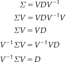
Thus, through the rotation and scaling of the eigenvector matrix, the original covariance matrix can be transformed into a diagonal covariance matrix, eliminating covariance altogether.
Equally significantly, if the eigenvectors are normalized, then the eigenvalues indicate the relative contribution of each of the eigenvectors to the covariance matrix. For large datasets, the relative weights provided by the eigenvalues can be used to reduce the dimensions of the data.
We will use an example.
Load the data file data.mat.
You’ll notice that the included matrix is a 50×3 matrix of data, corresponding to 50 samples of a three-valued vector quantity. Because this data has more than two dimensions, visualizing this data is fairly difficult. We will use PCA to remap the data to new axes that better represent the variance of the data.
First, we can use the MATLAB cov() function to generate the covariance matrix:
Next, we will calculate the eigenvectors of C:
The value of D shows the three eigenvalues. Note that one of the eigenvalues is far smaller than the other two (1.601e−03). This indicates that the corresponding eigenvector (column 2 of V) only weakly contributes to the covariance matrix. As a demonstration of this, we will apply the eigenvector matrix V to the original data and examine the data:
Note that these variances of the modified data set match the eigenvalues of the original covariance matrix. Just as important, the variance corresponding to the second axis is substantially smaller than the other two. Because of this discrepancy, we can omit this axis in the rotated data set while still preserving the variance of the original data.
3.3 Probability and Statistics
3.3.1 Introduction
The intent of this section is a brief, rapid introduction to probability and statistics and their use in MATLAB. This primer cannot hope to replace a good elementary statistics sequence. That said, those readers with a less extensive background in statistics may find this section useful. This primer expects a basic understanding of calculus and a passing familiarity with MATLAB, such as what might be expected by having gone through the introductory chapters of this very book.
3.3.2 Random Variables
Much of probability is built upon the concept of a random variable. A random variable is a variable that can take any one of a number of defined values and whose actual value is determined solely by chance. As a simple example, we will define a random variable X to represent the outcome of a flip of a coin, where the value 1 denotes an outcome of “heads” and a value of 0 signifies the outcome “tails.” With a fair coin, the probability of heads or tails is equal.
Usually, we will represent the probability of an outcome as a rational number, often a fraction. As a fraction, the numerator represents the number of outcomes that yield the event, and the denominator represents the total number of outcomes in the system. So, in the case of random variable X, the probability of a tails event is ![]() . There are two possible outcomes, and the event of getting “tails” is the result of only one. Similarly, the probability of a heads event is also
. There are two possible outcomes, and the event of getting “tails” is the result of only one. Similarly, the probability of a heads event is also ![]() . Together, the probability of a heads event or a tails event occurring is
. Together, the probability of a heads event or a tails event occurring is ![]() or 1. This should make sense, as flipping an idealized coin should yield one or the other.
or 1. This should make sense, as flipping an idealized coin should yield one or the other.
This property of probabilities, summing to one, is a general one, and in a formal treatment of probability is usually defined axiomatically. This usually includes three axioms:
1. Probability is always nonnegative.
2. The probabilities of all possible events sum to one.
3. The probability of any of multiple mutually exclusive (nonoverlapping) events is the sum of the individual event probabilities.
These three are also known as the “Kolmogorov axioms” and form the traditional axiomatic foundation of probability theory.
We can generalize the coin flip example by allowing the probabilities of the two outcomes to differ from ![]() . Under such a generalization, a random variable having two possible outcomes is called a Bernoulli random variable. Unlike the case of X, where we modeled a coin flip, a Bernoulli random variable does not necessarily have equal probabilities for the two outcomes. The probabilities for both must, however, sum to one.
. Under such a generalization, a random variable having two possible outcomes is called a Bernoulli random variable. Unlike the case of X, where we modeled a coin flip, a Bernoulli random variable does not necessarily have equal probabilities for the two outcomes. The probabilities for both must, however, sum to one.
Given a Bernoulli random variable Y, with probability p of outcome 1 and probability (1−p) of outcome 0, we denote the probability of an outcome 1 of Y as Pr(Y=1). Here, Pr(Y=1) would be equal to p. We can define a function f(y)=Pr(Y=y) such that the value of f(y) is the probability of value y of random value Y. In other words,

This function is termed the probability mass function (PMF) of random variable Y. It literally outlines where the mass of the probability of the variable lies.
Thus far, our example has focused on a single Bernoulli variable representing a single binary outcome. As a more complex example, we can flip a coin multiple times and count the number of heads. This can be represented as a sum of Bernoulli random variables. We can also define a new type of random variable, a binomial random variable, to represent this scenario.
Formally, given a series of n Bernoulli random variables ![]() , all with equal probability p of outcome 1
, all with equal probability p of outcome 1 ![]() , a binomial random variable Y represents the total number of positive (i.e., 1 valued) outcomes. We say here that n represents the number of trials. Since each trial must have either a positive or negative (i.e., zero-valued) outcome, the total number of positive and negative outcomes must equal the number of trials, and the number of negative (i.e., zero-valued) outcomes is n−Y.
, a binomial random variable Y represents the total number of positive (i.e., 1 valued) outcomes. We say here that n represents the number of trials. Since each trial must have either a positive or negative (i.e., zero-valued) outcome, the total number of positive and negative outcomes must equal the number of trials, and the number of negative (i.e., zero-valued) outcomes is n−Y.
Much like with Bernoulli random variables, we can define a probability mass function. However, because a binomial random variable has more outcomes, this case is more complex. Take a series of three coin tosses and a random variable Y representing the total number of heads the series of flips (see Table 3.1).
Table 3.1
This table shows the possible outcomes in a three coin flip experiment and the total number of heads in each outcome.
| Flips | Number of Heads |
| TTT | 0 |
| TTH | 1 |
| THT | 1 |
| THH | 2 |
| HTT | 1 |
| HTH | 2 |
| HHT | 2 |
| HHH | 3 |
There are now eight possible outcomes. This can be calculated quickly from 23=8. (Each flip occurs independently of the others and doubles the number of outcomes in the series. Thus, with 3 flips in the series, the total number of outcomes is 2×2×2=8.) Of these 8, only one outcome involves 0 or 3 heads. 1 or 2 heads both involve 3 outcomes. With this information and from this table, we can construct a probability mass function for Y.
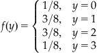
Values below 0 or above 3 were omitted as they are necessarily 0 (these already sum up to 1). In general, the probability mass function for a binomial random variable can be calculated from the formula
![]()
Here, n is the number of trials, p is the probability of a positive outcome on any one trial, and k is the number of successes or nonzero-valued results. The notation ![]() might look scary due to its unfamiliarity, but it is simply the number of combinations, also called the binomial coefficient, and it can be calculated from
might look scary due to its unfamiliarity, but it is simply the number of combinations, also called the binomial coefficient, and it can be calculated from ![]() . The MATLAB function C=nchoosek(n, k) will calculate the number of combinations automatically for you:
. The MATLAB function C=nchoosek(n, k) will calculate the number of combinations automatically for you:
For more complex distributions, a bar graph provides an excellent tool for visualizing a probability mass function. Figure 3.5 depicts the probability mass function for the probability of the total number of heads for eight coin flips. With the probabilities in the vector p, the command

produced the plot shown in Figure 3.5. (The expression 0:8 generated the markers for each bar at the bottom of the plot, denoting the number of successes.)
As n increases, you may notice that the probability mass function acquires a bulging shape, where success counts near the middle of the possible range have much higher probabilities relative to the probabilities of all heads or all tails. Descriptive statistics provides a number of standard terms that we can use to characterize the distribution.
We can describe the central tendency of the distribution. We will discuss three common ways of describing the central tendency of a distribution. The first is the mode. The mode is defined as the most probable outcome in the distribution. From a bar graph depicting a probability mass function, the mode is the outcome with the highest probability. The second central tendency is the median. The median is defined as the outcome corresponding to the point where the probability masses above or below the outcome are equal. This can also be stated as the outcome for which the cumulative probability is equal to or exceeds 0.5.
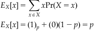
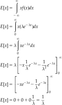
The final central tendency that we will discuss is the mean. Occasionally, the term expected value is also used to indicate the mean expected value. This term suggests an interpretation for the mean, given a binomial random variable Y drawn from a known distribution, what value should you expect? We can define the expected value of a function f(x) relative to a distribution for a random variable X as
![]()
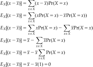
or, the expected value of a function f(x) is the value of the function at x multiplied by the probability of x, summed over all values x for the random variable X. The mean is defined as the expected value of the function f(x)=x. So, the mean of the three coin toss example discussed previously is

Clearly, the mean is not a valid number of successes (we cannot have a fraction of a coin flip). The mean is not guaranteed to be a valid count for the variable in question. Nonetheless, the empirical average of many trials or random variables will grow ever closer to the true mean of distribution, assuming that all trials originate from the same underlying distribution and are statistically independent. This property, that the empirical average over many trials will approach the expected value, is called the Central Limit Theorem.
We can easily demonstrate that the mean for any Bernoulli random variable with probability p of outcome 1 is p:
As mentioned earlier, the mean provides a measure of the central tendency. What the mean doesn’t provide is a measure of the dispersion of the data. One group of data may be widely dispersed, and another may be tightly clustered, but both may have very similar means.
Unfortunately, we cannot simply use the sum of the differences between the random variable and the mean as a measure of dispersion, as the positive and negative deflections around the mean tend to cancel each other out, tending toward an expected value of zero:
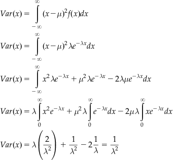
Instead, we can calculate the expected value of square of this difference (as they don’t cancel out), called the variance:

Thus, the variance is the difference between the expected value of the random variable squared and the square of the mean. Unlike the expectation of the difference between the random variable and the mean, the variance is rarely zero. Because the variance is in units equivalent to the square of the random variable, we will often use the standard deviation instead, which is defined as the square root of the variance. The Greek letter sigma is often used to represent standard deviation:
![]()
By definition, sigma squared represents the variance of the random variable.
3.3.2.1 Sample Estimates of Population Parameters
Often when dealing with real data the actual distribution of values will not be known. After collecting a set of data, one can look at the empirical distribution of the collected data. Is that distribution necessarily an instantiation of the exact distribution of the population from which the data was collected? Since each data point is a random variable in a sample that is often considerably smaller than the population it was drawn from, the empirical distribution of data will never match exactly, but (for most distributions) increasing numbers of samples will allow a better approximation of the distribution of the (usually much larger) population.
When we discuss sample estimates of a distribution, we use a slightly different notation from the notation we are used to for the actual distribution itself. The sample mean of a set of random variables is denoted as ![]() rather than
rather than ![]() . This mean of the sample forms an estimate of the mean of the actual distribution and is calculated from a sample by
. This mean of the sample forms an estimate of the mean of the actual distribution and is calculated from a sample by
![]()
or the sum of the values divided by the number of values. The estimate of the standard deviation is written as s instead of ![]() and is calculated as
and is calculated as

The estimated variance is the square of this quantity, and is written as s2. You may note the factor of N−1 rather than N as with the mean. This results from the use of the empirically calculated mean in the estimate for the standard deviation. Because of this factor, this value is often called the unbiased estimate of the standard deviation, as one degree of freedom is lost. Note that in practice you will almost always deal with sample estimates of these parameters, as you have access to a sample of data (sampled from the population at large, but not equal to that population).
MATLAB provides the functions mean(), var(), and std() to estimate the mean, variance, and standard deviation of a sample.
3.3.2.2 Joint and Conditional Probabilities
At this point, we’ve explored single variable distributions fairly extensively. While many phenomena can be modeled quite effectively with just a single independent variable, this is not always the case.
Take for example the following scenario: Instead of one, you are now rolling two ordinary six-sided dice on each trial. The total can be modeled as a single independent variable, but it may be simpler in certain cases to treat the dice as two separate random variables X and Y. Both variables would be from the same uniform discrete distribution, so we say these are identically distributed.
With two random variables, we can discuss the probabilities of outcomes across both of them at the same time. For example, P(x<2, y<3) is the probability that the result of the first die is less than 2 and the result of the second is less than 3. This can be computed by enumerating all the possibilities and determining the fraction that complies. In this case, the outcomes are (1, 1) and (1, 2), so there are two possible outcomes that meet the criteria. There are 36 possible outcomes, so the probability is 2/36. This probability over multiple variables is called the joint probability over X and Y.
You may have noticed a relationship between the probabilities of each individual case and the overall probability. In the context of multiple random variables, probabilities of individual random variables are termed marginal, for historical reasons (there is nothing inherently marginal about it; they were computed—manually—by writing probability sums in the margins of a probability table). Thus, the probability P(x<2) in this context is a marginal probability. For P(x<2), there is one outcome out of six (for X alone, only the first die is considered). Likewise, there are two outcomes where the die roll is less than 3, so P(y<3) is 2/6. The product of these two probabilities is equivalent to the joint: P(X, Y)=P(X)P(Y). This general relationship, where the joint probability is the product of the marginal probabilities, defines statistical independence. In other words, the outcome of X and Y do not depend on one another. As we’ve defined our problem, we can say that X and Y are independent and identically distributed (very frequently abbreviated as i.i.d.).
Many systems of variables will not be independent. If we take for example the previous system in the context of a random variable Z representing the total of X and Y, the joint probability is clearly not just the product of the individual probabilities. For example, take the events of rolling a 12 total, and rolling a 6 on the first die (before looking at the outcome of the second). In this case, P(x=6, z=12) is 1/36. However, the probability of rolling a 6 is 1/6 and the probability of rolling a 12 on the two dice is 1/36. Thus, the variables Z and X are not independent: the overall outcome rather strongly depends on what was rolled on the first die.
Given the relationship between X and Z, we may want to express probabilities of certain events conditioned on other events having occurred. For example, if the first die comes up 6, what is the probability that the total will be 12? (Hopefully, it is clear that the probability of that total is 1/6, the probability of rolling a 6 with the remaining die. This holds because the two die themselves are independent. This might seem confusing, but it is important to keep in mind separately.) We can use a conditional probability to express such cases. A conditional probability takes the form P(A|B), which is the probability of outcome A, given that B has occurred. So, the previous example of rolling a 12 given one die is already 6 can be written as P(z=12|x=6).
The joint, conditional, and marginal probabilities have the relationship
Thus, the joint probability of events A and B happening is equal to the conditional probability of A occurring if B occurs multiplied by the probability of B occurring. We can verify this in the case of the two-die scenario.
We know that the probability of P(z=12, x=6) is 1/36, from the above. P(x=6) is 1/6 (remember, this is the probability of the first die coming up 6 considered entirely on its own). As discussed above, P(z=12|x=6) is also 1/6. Thus, the relationship holds true. It is important to remember that this relationship holds even when the random variables are not independent.
A serious drawback of using dice examples in most introductory treatments of probability is questionable relevance. It is understandable why these examples are used so often; a tightly constrained problem allows for establishing the concepts with great mathematical precision. However, most of us are hopefully not spending the majority of our days throwing dice. Introducing real world examples is dicey, as most real world examples map onto such fundamental concepts in multiple ways. No matter which topic you pick, this holds; you will imply a relationship (sometimes a causal relationship) between variables that can a priori be conceptualized as independent. But that is what science is all about: finding these relationships.
Ultimately, a conditional probability indicates that additional information is known about the problem space. Science establishes this information; society uses it beneficially. For instance, an insurance company might assess your risk of dying within the next 10 years differently if they knew that you are overweight, smoke, and don’t exercise. In a way, all of life is about harvesting the information expressed in conditional probabilities, and optimizing one’s outcomes in the face of uncertainty. It is now cliché that half of marriages end in divorce. It is less well-known that there are pretty solid conditional probabilities involved; the outcome strongly depends on educational and financial status as well as number of previous sexual partners. Put differently, while the probability of divorce for any couple selected randomly is around 0.5, the conditional probability can be far from 0.5 under certain conditions.
Another common situation arises in a medical context. For instance, the probability of a baby to have Down’s syndrome is about 1/700. However, the conditional probability is as high as 1/20, given that the mother is over 45 years old. Similarly, the conditional probability that a child will develop autism is four times higher than the unconditional probability if it is known that the child is male.
We can also expand our understanding of expectation and variance to account for multiple random variables. Conditional expectation follows in a straightforward way from conditional probabilities. So, to use the previous two-die example, the expectation of the sum Z is 7:
![]()
We can calculate the conditional expectation of the sum Z given that the first die roll is a 6 in a similar manner:
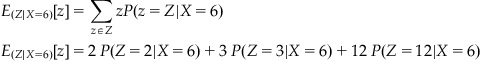
For any values of Z less than 7, the conditional probability is zero, and the corresponding terms drop out, leaving
![]()
With one die known, only one outcome of the six possible can produce each sum, so
![]()
For systems with multiple random variables, a single variance does not sufficiently describe dispersion. The term covariance describes variance that occurs together between random variables, due to statistical dependence. Covariance between two variables is defined as
![]()
over the two variable expectation. Covariance is often written as ![]() . When calculated between a variable and itself, the covariance is equivalent to the standard variance, sometimes written as
. When calculated between a variable and itself, the covariance is equivalent to the standard variance, sometimes written as ![]() . A nonzero covariance indicates some interdependence between the two variables. Two entirely independent variables should have a covariance of zero.
. A nonzero covariance indicates some interdependence between the two variables. Two entirely independent variables should have a covariance of zero.
3.3.3 The Poisson Distribution
The Poisson distribution is used to describe phenomena that are comparatively rare. In other words, a Poisson random variable will relatively accurately describe a phenomenon if there are few “successes” (positive outcomes) over many trials.
The Poisson distribution has a single parameter, ![]() . For a Poisson distribution modeling a binomial phenomenon,
. For a Poisson distribution modeling a binomial phenomenon, ![]() can be taken as an approximation of np.
can be taken as an approximation of np.
Aside from use as an approximation for the binomial distribution, the Poisson distribution has another common interpretation. For an infrequently occurring event, the parameter lambda can be viewed as the mean rate, or ![]() , where n is the mean events per unit time, and T is the number of time units. In such a case, a Poisson distribution with the appropriate parameter
, where n is the mean events per unit time, and T is the number of time units. In such a case, a Poisson distribution with the appropriate parameter ![]() will approximate the distribution of events over time or the number of events in an interval.
will approximate the distribution of events over time or the number of events in an interval.
Events whose occurrence follows a Poisson distribution have another interesting property. Given a series of Poisson distributed independent random variables ![]() and their corresponding arrival times
and their corresponding arrival times ![]() , we can calculate the distribution of the corresponding inter-event intervals.
, we can calculate the distribution of the corresponding inter-event intervals.
Let N(t) equal the number of events at some time t, where P(k=N(t)) follows a Poisson process with parameter ![]() . Then, the probability of the nth event occurring at
. Then, the probability of the nth event occurring at
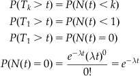
Likewise, we can calculate a distribution for the inter-event intervals. Here, the probability of an interval between two successive events Tk and Tk−1 being larger than some time t is the same as the probability of exactly k−1 events occurring within the interval 0 to ![]() . This can be expressed as follows:
. This can be expressed as follows:
![]()
The probability of k−1 events during the interval ![]() is equivalent to the probability of no events during the interval 0 to t.
is equivalent to the probability of no events during the interval 0 to t.
![]()
By definition, k−1 events occurred during the interval 0 to Tk−1. Thus, if any events occur during the interval Tk−1 to ![]() , this would mean that the number of events in the interval
, this would mean that the number of events in the interval ![]() would not be k−1 but greater than k−1.
would not be k−1 but greater than k−1.
This implies that the intervals are distributed in a “memoryless” fashion. In other words, for an ongoing process following a Poisson distribution of events, the distribution of waiting time to the next event does not change over time. Put differently, knowing when the last event occurred does not give you any information about when to expect the next one.
The distribution of intervals that we have derived here is called the exponential distribution. This is our first example of a continuous distribution. Unlike with discrete distributions, calculating the exact probability of a single value in a continuous distribution is not feasible, as it is always zero. To understand why, one can use the previous example of the exponential distribution of time intervals for a Poisson process. The probability of a specific value, say 3 seconds, would correspond to the probability of the time interval being exactly equal to 3 seconds. Since this would exclude any interval even infinitesimally close to 3, this will be vanishingly small regardless of the number chosen. Therefore, when working with continuous probabilities, we compute the probability of a variable falling within a range of values.
Because of this fundamental difference, continuous distributions do not have a probability mass function like discrete distribution. Continuous distributions are defined in terms of cumulative distribution functions. The derivation of the exponential distribution above provides an excellent example. Above, the probability of an inter-event interval T being greater than some value t was found to be equal to ![]() . Usually, the cumulative distribution function F is defined as the probability of a random variable being less than a given value. Following those conventions, the cumulative distribution function F for the exponential distribution can be defined as
. Usually, the cumulative distribution function F is defined as the probability of a random variable being less than a given value. Following those conventions, the cumulative distribution function F for the exponential distribution can be defined as
![]()
(This falls out of the requirement that the sum of probability be equal to one. If ![]() .)
.)
To determine the probability of a random variable falling within a specific range, we can subtract ranges. For example, the probability of a random variable T falling between t1 and t2 can be expressed in terms of each value alone:
![]()
This holds true because the probability of the random variable T being less than t2 includes all cases where the random variable is less than t1. So, the probability mass corresponding to ![]() must be subtracted out.
must be subtracted out.
This can be more clearly understood by introducing the probability density function, a function f(x) such that the cumulative distribution function ![]() . For a probability expression with a density function f(x), the probability
. For a probability expression with a density function f(x), the probability ![]() . Likewise, the range
. Likewise, the range ![]() .
.
Exercise 3.15
Demonstrate through derivation that the probability density function f(x) for the exponential distribution is ![]() . Remember that the cumulative density function is defined in terms of the probability density function as
. Remember that the cumulative density function is defined in terms of the probability density function as ![]() and the cumulative density function for the exponential function as given above. (Note: Because the exponential distribution is only defined for non-negative numbers, the lower bound of the integral can be set at 0.)
and the cumulative density function for the exponential function as given above. (Note: Because the exponential distribution is only defined for non-negative numbers, the lower bound of the integral can be set at 0.)
Continuous distributions also have expectations like discrete distributions. Instead of summing over all probabilities, the expectation is defined in terms of an integral over the probability density function. For a probability density function f(x), the expectation of the function g(x) is defined as
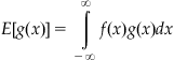
With this, we can calculate the mean and variance for the exponential distribution:
3.3.4 Normal Distribution
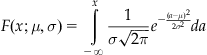
The last classical distribution that we will discuss here is the normal distribution. There are many more, some of which will be visited in later chapters for more specialized purposes. Because its cumulative distribution function is not solvable analytically, the normal distribution is usually defined in terms of its probability density function,
![]()
Here, the parameters μ and σ define the mean and standard deviation of the distribution. A normal distribution with μ=0 and σ=1 is called a standard distribution.
The cumulative distribution function of the normal distribution is the integral over all values x:
The cumulative distribution function of the standard distribution is often denoted as ![]() . This cumulative distribution function is often defined in terms of another special function whose form is very similar to the integral over the probability density. This function is commonly called the error function
. This cumulative distribution function is often defined in terms of another special function whose form is very similar to the integral over the probability density. This function is commonly called the error function ![]() . So, in terms of the error function, the cumulative distribution function of the standard distribution is
. So, in terms of the error function, the cumulative distribution function of the standard distribution is ![]() .
.
MATLAB defines both a cumulative distribution function, normcdf(x, mu, sigma), and the error function, erf(x), for the normal distribution.
The normal distribution approximates how many phenomena vary. In particular, the normal distribution is useful in understanding error.
3.3.5 Confidence Values
The normal distribution is particularly useful because of the central limit theorem. Given N independent, identically distributed random variables with mean ![]() and variance
and variance ![]() , the central limit theorem asserts that the distribution of the mean of the random variables will converge to a normal distribution with mean
, the central limit theorem asserts that the distribution of the mean of the random variables will converge to a normal distribution with mean ![]() and variance
and variance ![]() . The dependency of the variance on the number of variables (in this case, samples) is particularly important. As we will see, this result is especially relevant to estimating distributions from samples.
. The dependency of the variance on the number of variables (in this case, samples) is particularly important. As we will see, this result is especially relevant to estimating distributions from samples.
Exercise 3.16
Here we will explore how the precision of a mean estimate varies with the sample count.
The use of randn(2^N(n), 100) here selects 2^N×100 samples from a standard normal distribution. The intent is to simulate picking 2^N samples 100 times in order to estimate the variance of the distribution of the means. mean() calculates the sample means, returning a vector of length 100, and var() estimates the variance of the distribution of means.
You should see a figure like
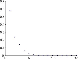
Figure 3.6
How does variance vary with sample count? How many more samples are required to halve the variance in the estimate of the mean?
The term standard error of the mean (or just standard error) is defined as
![]()
where s is the estimate of the standard deviation and n is the number of samples in the estimate.
Often, the error will be expressed as confidence intervals around the mean. A confidence interval is expressed as the interval surrounding the mean within which an estimate of the mean should fall with a certain probability (often 90% or 95%). For a 95% confidence interval, this is approximately 1.96 times the standard error on either side of the mean estimate.
For example, let’s assume we have a normally distributed population whose actual mean is 25 and whose variance is 5. We can collect a sample of 10 as follows.
In this case, the 95% confidence interval around the mean estimate 25.5606 would be 24.1473 to 26.9739.
For values other than 95%, we can calculate the factor of the standard error directly using the MATLAB function erfinv(). erfinv() calculates the inverse of the error function discussed earlier. To determine the factor to replace the 1.96, you will need to calculate ![]() , where p is the confidence interval probability. It is important to note that this assumes normally distributed values.
, where p is the confidence interval probability. It is important to note that this assumes normally distributed values.
3.3.6 Significance Testing
Hand in hand with the idea of a confidence interval is significance testing. Take a known distribution: a normal distribution with a mean of 15 and a standard deviation of 3. A sample of five values has a mean of 11. Is this sample likely to be drawn from the same population? How about a sample of 100 values with the same mean? There is always a chance that the sample was drawn from the distribution. The question is, with which probability? Significance testing provides systematic methods for answering such questions.
Returning to the original question posed about the estimated sample mean of 11, we can describe this in a probabilistic way; in fact, we can rephrase this probabilistically in at least two ways. First, we can ask how probable a mean of 11 or lower might be, or
![]()
Secondly, we can ask how probable a mean at least as extreme as 6 might be, or
![]()
Classical statistics distinguishes these two refinements of our original questions as a hypothesis test: we use the properties of the distribution to test a null hypothesis (often written as H0) that the five item sample is drawn from the known distribution. An extremely low probability of such an extreme result would argue against the null hypothesis or, alternatively, for rejecting the null hypothesis.
Typically, a maximum threshold for the probability is chosen, called the significance level. Common values are 1%, 5%, and occasionally 10%. Outcomes with probabilities below the significance level are termed statistically significant at the corresponding level, and usually strongly argue for rejecting the null hypothesis. It is important to keep in mind that hypothesis testing is only evidence for or against rejecting the null hypothesis. For example, a significance level of 5% indicates that only one out of every twenty repetitions would produce a result as extreme. If an experiment is repeated 20 times, on average, the outcome would be statistically significant once. All that the p value gives you is the probability that such data so extreme (or more extreme) could happen by chance, assuming that the null hypothesis is true. By this logic, if the significance level is not met, it does not mean that the null hypothesis is true, just that we failed to reject it at this significance level.
Often, a significance level is selected prior to analysis or even the collection of data, and a significance of 5% is especially common. The selection of a significance level requires a tradeoff between two types of error. Choosing a less stringent significance level increases the risk of interpreting a result as indicating that the null hypothesis should be rejected when it’s not actually false (this is classically called a Type I error and refers to spurious findings). Alternatively, a more stringent significance level enforces a more severe threshold for the rejection of the null hypothesis, but setting too low a significance level can miss rejection when the null hypothesis is actually false (a classical Type II error: missing differences that are really there). How one should pick the significance level depends on the relative value of the outcomes in a given practical case: how serious is it to miss real effects versus how serious it is to claim the existence of effects that are not really there. More than the brief treatment of Type I/II errors here is beyond the scope of this primer, and the reader is referred to a more detailed reference for an in-depth discussion.
Significance tests can be classified as one-tailed or two-tailed hypothesis tests. The origin of these names can be easily understood from an illustration of the expected distribution of sample means. From the central limit theorem, as discussed in the last section, we know that sample means from the known distribution should vary with a normal distribution whose mean matches that of the underlying distribution and whose standard deviation is ![]() .
.
Figure 3.7 shows the expected PDF (remember, probability distribution function) for sample means for samples with five elements. Shaded is the probability of the sample mean having a value at least as extreme as the collection value. Figure 3.8 shows the shaded portion of the PDF in greater detail. (Noting that ![]() may help in understanding Figure 3.8.)
may help in understanding Figure 3.8.)

Figure 3.7
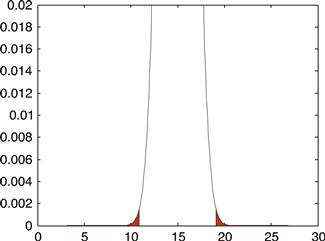
Figure 3.8
Figure 3.9 shows the same PDF with the probability of the sample mean being less than 11 shaded. In this case, the shaded probability covers only one of the two ends of the PDF. This is a one-tailed test. Likewise, the previous case covering both tails of the PDF is called a two-tailed test.
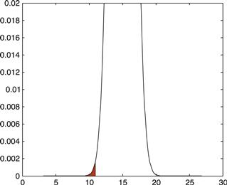
Figure 3.9
Using significance testing correctly requires determining whether the question at hand involves a one-tailed or two-tailed test. Here we are interested in ascertaining whether the measured sample comes from the known distribution. Understanding the extreme nature of the sample mean is what we’re interested in, so a two-tailed test is most appropriate.
Since the sample mean should be distributed according to a known normal distribution, we can calculate the two-tailed probability using the MATLAB function normcdf. Recall that normcdf(x, mu, sigma) returns the cumulative distribution function at x for a normal distribution with ![]() =mu and
=mu and ![]() =sigma.
=sigma.
Next, we can calculate ![]() . normcdf() can be used for this as well, but if the same procedure is followed with 19 substituted for 11, we will calculate
. normcdf() can be used for this as well, but if the same procedure is followed with 19 substituted for 11, we will calculate ![]() :
:
Note that the value here is substantially larger than the probability of the first tail. To calculate ![]() , we can use the equality
, we can use the equality ![]() :
:
This matches the probability mass of the first tail, as one might expect from Figure 3.9. The sum of the two is the probability that the sample mean is at least as extreme as the estimated mean here:
So, roughly 3% of the time, the empirical mean of five samples from the known distribution would be at least as extreme as 11. At the 1% significance level, this would not provide sufficient support for rejecting the null hypothesis, but it would at the 5% level.
3.3.6.1 Student’s t Distribution
Imagine an electrophysiology experiment attempting to determine whether a single neuron responds to a stimulus. In trials without the stimulus, you see firing rates as in the second column of Table 3.2. The third column of the table shows the firing rates in trials with the stimulus. Obviously, we’re interested in whether the stimulus alters the firing rate. This question can be rephrased as a statistical test: what is the probability that the two distributions are the same or, rather, that two these samples were drawn from the same distribution?
Table 3.2
| Trial | Rate without stimulus | Rate with stimulus |
| 1 | 54.5 | 67.1 |
| 2 | 43.5 | 63.8 |
| 3 | 36.5 | 73.5 |
| 4 | 48.7 | 57.2 |
| 5 | 41.8 | 31.0 |
| 6 | 52.6 | 54.2 |
| 7 | 28.7 | 33.1 |
| 8 | 57.1 | 117.0 |
| 9 | 40.5 | 71.4 |
| 10 | 48.2 | 133.8 |
| 11 | 57.3 | 60.0 |
| 12 | 50.8 | 41.1 |
| 13 | 62.5 | 93.0 |
| 14 | 30.8 | 33.5 |
| 15 | 28.9 | 52.0 |
Unfortunately, since we don’t know either of the distributions from which the firing counts are sampled, we can’t use the procedure we used in the previous section. This will often be the case in real scenarios. Fortunately, a wide variety of tests for general purpose significance testing have been defined. For example, Student’s t test is appropriate here.
Student’s (actually William S. Gosset, but being in the employ of Guinness, he had to publish under a pseudonym) t test (Student, 1908) is useful in a number of statistical scenarios. Here, we will use a paired t test. In this experimental paradigm, the measurements of firing rate with and without the stimulus are not independent (the experiment measures the same cell under two different conditions). We can pair the measurements before and during stimulus presentation, and use the t test to determine whether the data is significantly different.
Under the paired t test, we need to calculate a t statistic from
![]()
where ![]() is the mean of the difference between elements of each pair,
is the mean of the difference between elements of each pair, ![]() is the estimated standard deviation of the differences between elements of each pair, and N is the number of pairs. Then, we need to use a Student’s t distribution in much the same way we used a normal distribution in the prior section. It is worth nothing that the t distribution is very similar to the normal distribution anyway, just with heavier tails to account for unknown population variance with small sample sizes.
is the estimated standard deviation of the differences between elements of each pair, and N is the number of pairs. Then, we need to use a Student’s t distribution in much the same way we used a normal distribution in the prior section. It is worth nothing that the t distribution is very similar to the normal distribution anyway, just with heavier tails to account for unknown population variance with small sample sizes.
MATLAB offers a number of functions to simplify this process. The function ttest() has two forms that are particularly used. ttest(x,y) performs a paired t test. This would be easiest if we have vectors x and y for the two samples.
>> x = [54.5 43.5 36.5 48.7 41.8 52 6 28.7 57.1 40.5 48.2 57.3 50.8 62.5 30.8 28.9];
>> y = [67.1 63.8 73.5 57.2 31.0 54.2 33.1 117.0 71.4 133.8 60.0 41.1 93.0 33.5 52.0];
Without specifying return parameters, ttest() performs a test and returns whether the null hypothesis should be rejected at the default significance level (5%). Thus, the data supports rejecting the null hypothesis that the stimulus has no effect on the firing rate. (In other words, the data suggests that the stimulus has an effect on the firing rate at the 5% significance level.) We can supply a different significance level as a final parameter to ttest():
This implies that the data does not support rejection of the null hypothesis at the 1% level of significance. Depending on the criteria of the experiment, significance at the 5% level may be sufficient, or a lack of significance at the 1% level may suggest that the experiment had insufficient “power” to detect an effect at this level, and more data should be collected to yield this power.
We can obtain the exact probability of the result or one more extreme by supplying a second return parameter:
If we have the differences between the sample pairs already calculated, we could also use another form of the ttest function. With a single vector, ttest(x) tests against a mean of 0. This is appropriate when we just have the differences between the pairs, not the actual values.
3.3.6.2 ANOVA Testing
Student’s t test covers a number of hypothesis scenarios for testing the results of a single factor (one independent variable) and between pairs of samples. Multiple samples or multiple experimental factors create a scenario that is difficult for a single t test to handle. To use a t test under such circumstances, we would need a separate t test for each distinct pair in the experiment. For a five factor experiment, this would require 25=32 separate tests! Note that on a significance level of 5%, we would expect 1 in 20 differences to test positively just by chance, even in the absence of any real experimental effects, so we would also have to adjust our significance level for multiple comparisons. If this sounds like a recipe for disaster, it is. An alternative approach for the statistical treatment of experimental data from experiments with more than one independent variable is the so-called “analysis of variance.”
An analysis of variance (ANOVA) allows us to ask the probability that a group of samples all originate from the same larger population without the inflated risk of a Type I error as with multiple t tests. As an example, we’ll expand our hypothetical experiment to three different stimuli. For simplicity, we will call them A, B, and C (see Table 3.3).
Table 3.3

First, we need to calculate the variance across groups.
>> stim_a = [39.2 45.7 45.9 42.8 60.2 50.7 39.9 50.8 43.0 55.9];
>> stim_b = [43.2 56.7 32.8 61.2 54.6 44.6 53.2 43.3 35.1 53.7];
>> stim_c = [66.5 54.5 62.6 45.6 46.8 34.9 53.3 60.1 69.7 61.0];
This requires calculating the mean for each stimulus
and the weighted sum of the squares of differences between the overall group mean and the mean of each group
Next, we need to calculate the variance within each group. We sum the squares of the differences between each measurement and its difference from the mean of its corresponding group:
We use these two values, the mean square difference between groups and the mean square difference within groups, to calculate the test statistic, f:
What does this tell us? If all three sets of data follow the same distribution, the distribution of f should follow an F distribution, which has two parameters. A discussion of the analytic form of the F distribution is beyond the scope of this text. For the purposes of our use of the F distribution, the two parameters are equivalent to the degrees of freedom in our data set: the number of stimuli minus one (3−1=2) and the total count of data points, minus the number of stimuli (30−3=27).
In this case, we need to determine the cumulative probability function for the F distribution given our f value and the two parameters. The fcdf() function will calculate this value.
This p value, 0.651, indicates a little over 65% of the time samples consistent with the null hypothesis (i.e., all distributed similarly) would yield an f value at least this extreme. Thus, we cannot discount the null hypothesis here.
3.3.7 Linear Regression
Assume two variables x and y, with an expected linear relationship between them such that ![]() . Under this relationship, we will call the y the dependent variable and x the independent variable. Let’s say that we have collected sample pairs
. Under this relationship, we will call the y the dependent variable and x the independent variable. Let’s say that we have collected sample pairs ![]() and want to estimate the parameters
and want to estimate the parameters ![]() (constant offset) and
(constant offset) and ![]() (slope) so that we can express y as a function of x.
(slope) so that we can express y as a function of x.
This estimation procedure is called linear regression (think “prediction”). Here, we are regressing x onto y. Under traditional terminology, as the independent variable, x is the regressor (plural: regressors). We can approach the estimation problem as a search for values of ![]() (we will call these estimates
(we will call these estimates ![]() ) that minimize the distance between the predicted value
) that minimize the distance between the predicted value ![]() and the actual measured value
and the actual measured value ![]() . The distance for each measured pair can be represented as
. The distance for each measured pair can be represented as
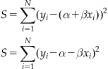
Then, the estimates ![]() can be calculated from the partial derivatives of S:
can be calculated from the partial derivatives of S:

The estimate ![]() can be calculated in the same manner:
can be calculated in the same manner:
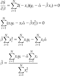
This has yielded a pair of equations in ![]() . The equation for the estimate of
. The equation for the estimate of ![]() can be substituted in and a closed form solution for
can be substituted in and a closed form solution for ![]() obtained:
obtained:
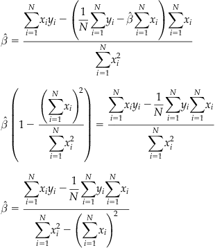
This method of linear regression is called least squares optimization, because the estimates originate from optimizing (here, minimizing) the sum of the squared distance.
Exercise 3.18
Write a MATLAB function that calculates estimates for ![]() , given two vectors of data: [a,b]=least_squares(x, y). Test against the following observations, where x is the independent variable, and y is dependent.
, given two vectors of data: [a,b]=least_squares(x, y). Test against the following observations, where x is the independent variable, and y is dependent.
Once an estimate is calculated, one should look at the residuals, the difference between the values predicted by the estimated parameters in the regression equation and the measured values. Assuming that the estimates for ![]() are stored within MATLAB variables a and b respectively, the residuals for a single variable can be calculated with
are stored within MATLAB variables a and b respectively, the residuals for a single variable can be calculated with
After any linear regression, it is important to review the residuals. In a perfectly linear relationship between dependent variables and regressors, the residuals will be randomly distributed (and ideally small). This implies that the difference between the prediction and measured value is primarily the result of error and not an additional nonlinear relationship.
After fitting, we can also look at the coefficient of determination, r2.
![]()
Here the numerator is the sum of the squares of the residuals, and the denominator is the sum of the squares of the difference between the dependent variable and its mean, essentially N times the var(y). Thus, given estimated parameters in MATLAB variables a, b, we can calculate r2 with
The coefficient of determination ranges from 0 to 1, with values near 1 indicating a better fit to the data. One interpretation of r2 is the proportion of variance explained by the model. Thus, a value closer to 1 indicates that most of the variance in the dependent variables originate in the variation of the regressors, as propagated through the model. A lower r2 implies that the dependent variables have some variance unaccounted for by the model.
Instead of calculating the estimates and coefficient of determination by hand, we can use the MATLAB function regress() in the Statistics Toolbox.
regress can perform multivariate linear regression, so for a single variable, x should be an N×2 matrix, where N is the number of observations. The first column data are the single variate observations, and the second column data consists of ones to indicate the constant offset. regress() returns a vector b with the estimates for the coefficients, ![]() . regress() also returns 95% confidence intervals for the coefficients in bint. regress() will also return the residuals if a third return parameter, r, is included.
. regress() also returns 95% confidence intervals for the coefficients in bint. regress() will also return the residuals if a third return parameter, r, is included.
3.3.8 Introduction to Bayesian Reasoning
Briefly put, Bayes’ theorem allows you to invert conditional probabilities if the base rates (or priors) are known. Illustrating the perils of eponyms, Thomas Bayes, a Presbyterian minister who first worked out the basic idea (but never published it), would probably be surprised by the attribution, in light of his other work.
When would one want to invert conditional probabilities? Surprisingly often. As a matter of fact, an awareness of Bayes’ theorem is likely much more useful in contributing to everyday wisdom in decision making than, say, calculus (which doesn’t stop the professionals from making up contrived examples anyway). This is due to the fact that it is often much easier to measure the conditional probability of one, but not another (yet related) event. If this appears too abstract, it is. A plastic example might help.
A country that shall remain unnamed has suffered a recent spate of vicious and unprovoked terrorist attacks on civilians. You have been hired by the government of this country to advise on a rational response to this unacceptable barbarism. Specifically, the question is whether the government should implement profiling measures against the known characteristics of the perpetrators, and if so, to what degree.
All terrorists have been bearded. This translates to p (Bearded|Terrorist)=1.
One in a million people is a terrorist. This translates to p (Terrorist)=0.000001.
One in 5 people is bearded. This translates to p (Bearded)=0.2.
And that’s all she wrote. In reality, having solid numbers on this is probably a better position than most governments can manage, so you are in a strong position.
What you really would like to know is the probability that someone is a terrorist given that he is bearded, but you only have the probability that someone is bearded if you already know he is a terrorist. This doesn’t help. If you already know someone is a terrorist, they might either already have committed their heinous act, or are in hiding. Language can be misleading here. Even though the probability that someone is bearded is 1, given that they are a terrorist, being bearded and being a terrorist are not synonymous in this case. Intuitively, if they were, there would have to be many more terrorists around (more than 1 in a million), given that 1 in 5 people is bearded. But how much is the risk of being a terrorist increased, given that someone is bearded?
Here, Bayes comes to the rescue.
In other words, the probability is 5 millionth. To put this in perspective, the absolute probability that someone is a terrorist if he is bearded is extremely low, while the relative probability is 5 times higher. This makes sense, as we use strong diagnostic information to link the two (as p (Bearded|Terrorist) is 1) and the base rate of bearded people in the country is 1 in 5.
You can now either advise the government that each bearded person should be scrutinized 5 times as much as a non-bearded person (to match the increased risk), or forgo profiling altogether, as the absolute risk is still so negligibly small. Both responses are rational.
What if the probability of being bearded given that someone is a terrorist was only half as strong—0.5? In other words, there are other kinds of terrorists around, they are not all bearded.
Plugging in the numbers yields
This makes sense. As the strength of the diagnostic information declined, the value of the criterion of beardedness to indicate terroristic tendencies declined in kind.
What if beardedness was much rarer; say only one in a hundred thousand people is bearded (and the strength of the link was back to 1)?
Now there is a 10% absolute chance that the person is a terrorist, just by virtue of being bearded, and the a priori chance is increased a hundred thousand-fold. Now, this seems like a rational case for strong profiling measures.
This admittedly somewhat contrived example was used to provide an intuitive feel for Bayesian statistics, using a striking and emotional case study.
While it is unlikely that you will be hired by a government in this position, it is far from unlikely that you will encounter Bayesian reasoning in your study of the neural and cognitive sciences. As a matter of fact, it has been suggested that the entire sensory apparatus of the brain works as one giant Bayesian machine. It would make sense that it might, as Bayes’ theorem allows making use of previous experience (establishing base rates) in a rational fashion. It has been shown that people do use prior experience to gauge what to expect from future interactions with members of a given class.
Moreover, the value of Bayesian reasoning is obvious in everyday life. It helps to know it. “Experts” might give misleading answers. For instance, if you go to the doctor for an AIDS test or a mammogram, you are not interested in the probability that the test is positive if you have the disease. You are interested in the probability that you have the disease if the test is positive! It has been conclusively shown that doctors frequently confuse these two probabilities, and give you wildly inaccurate odds (Gigerenzer and Hoffrage, 1995; Hoffrage and Gigerenzer, 1998). This concludes our introduction to Bayesian Reasoning—as well as our Mathematics and Statistics Tutorial for the purposes of this book. If you are interested in specific applications of Bayesian Reasoning in neuroscience, see chapter 22. For a more extensive treatment of Bayes’ theorem and Bayesian inference, see MacKay (2003).
3.3.9 Outlook
There is an almost infinite number of concepts we could add at this point. We could discuss other distributions, such as the Chi-squared distribution. We could take Bayes one step further and talk about likelihood modeling. However, this will suffice as a conceptual introduction to mathematical and statistical fundamentals. Some of these issues, e.g., maximum likelihood estimations, will be revisited in later chapters where appropriate. For now, we feel that enough groundwork has been laid, and that—if you have been working with us through this material—it is solid enough to carry you through the next chapters, which is really all anyone can ask for.