
Neural Data Analysis II
Binned Spike Data
Pascal Wallisch
Linear models have limitations for modeling observed neural data. In this chapter, we will examine a simple nonlinear encoding model which can model discrete, non-negative data obtained by counting the number of spikes occurring in a given time bin. Luckily, the nonlinear encoding model introduced here can be fit using a built-in function available in MATLAB®.
Keywords
exponential function; Poisson distribution; log-linear models; peri-event time histogram
18.1 Goals of this Chapter
Previously, you used a simple linear encoding model to predict a neuron’s firing rate, obtained by averaging over many trials for a range of stimuli. However, linear models have limitations for modeling observed neural data. In this chapter, we will examine a simple nonlinear encoding model which can model discrete, non-negative data obtained by counting the number of spikes occurring in a given time bin. Luckily, the nonlinear encoding model introduced here can be fit using a built-in function available in MATLAB®.
18.2 Background
In the last chapter, you saw that a cosine tuning model does a good job of describing the firing rate (averaged across many trials) of a neuron as a function of direction. In particular, you saw that neurons have a baseline firing rate, a preferred direction where the firing rate is at its maximum, and an anti-preferred direction where the firing is at its minimum. When the cosine tuning model is expressed as a sum of a sine and cosine (see the end of Section 17.3.4), then the model can be fit using linear regression and the MATLAB function regress. Linear regression may not always be the best choice, as it makes certain assumptions about the raw data. For example, linear regression assumes data are continuous. However, our data consists of timestamps, and our binned data are counts of the number of spike timestamps that fall within a given bin. What does this mean? To start with, we know that a count is always non-negative.
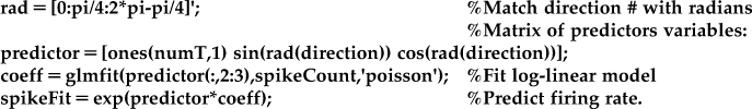
Load the data for this chapter. This data was also collected during the eight-target center-out task, and the data is formatted the same as the data from Chapter 17. Start by constructing the empirical tuning curve for neuron #2, as we did in Chapter 17, and fit it to the standard cosine tuning model. If you do this, you will end up with a plot like Figure 18.1. The interesting thing about this neuron is that it has a lower baseline firing rate than previous neurons we have examined. The neuron does increase its firing rate for its preferred direction (around 315 degrees), but because it cannot fire less than zero spikes per second, it fires minimally for a wide range of directions (90, 135, 180, and 225 degrees). When the standard cosine tuning model is fit to this data, it does not fit the peak firing rate well, and it predicts a negative firing for the anti-preferred direction of 135 degrees. Obviously, this is not an adequate model for this neuron.

18.2.1 Exponential Function
What we need is a function which can only predict nonnegative firing rates. One such function is the exponential function, ex. If x is one, the value of this function is simply e, or approximately 2.718. If x is zero, the function is 1, and as x becomes more negative, the function will approach but never reach zero. In MATLAB, the exponential function is exp. To deal with low-firing neurons, we simply need to apply the exponential function to the cosine tuning model we used in the last chapter:
The mean firing rate can be fit as before, and now the prediction is quite good (see Figure 18.2).

However, we are doing something a little odd here by averaging the firing rates before fitting the function. It means that we are weighting data from each direction equally, even though the number of trials completed in each direction is not exactly equal (there are 71 trials for direction 4, but 48 for direction 5). A better approach would be to fit the raw data from each single trial, which consists of counts of how many times the neuron spiked in certain time windows. Thus the raw data is nonnegative and discrete. Using linear regression on discrete data is usually not appropriate, because linear regression assumes that the data is continuous, and that the relationship is disturbed by Gaussian noise.
18.2.2 Poisson Distribution
A better choice is to assume that a discrete count follows a Poisson distribution. This is a simple but useful discrete distribution, which is good for modeling the number of events which occur in small amount of time or space. For example, the Poisson distribution might be used to model how many phone calls a call center might receive in an hour, or the number of grass seeds which sprout in a small patch of earth. Here, we use it to model the number of spikes detected in a given time bin. The use of the Poisson distribution for modeling spike trains is discussed in more detail in Chapter 33. We will compare the distribution of spikes we actually observe to what is expected with the Poisson distribution. We first need to collect the raw spike count in a 2-second window centered on the go cue for each trial:
| neuronNum=2; | %Select which neuron we want |
| numT=length(direction); | %Count number of trials |
| spikeCount=zeros(numT,1); | %Initialize count vector |
| for ii =1:numT | |
| centerTime=go(ii); | %Find go cue for given trial |
| allTimes=unit(neuronNum).times-centerTime; | %Center spike times on go |
| spikeCount(ii)=sum(allTimes>-1 & allTimes<1); | %2 seconds window |
| end |
We now have a vector of the raw spike counts for each trial. Take a look at the distribution of spike counts for direction two:
| dirNum=2; | %Select the direction we want |
| indTemp=find(direction==dirNum); | %Find appropriate trials |
| spikeTemp=spikeCount(indTemp); | %Pick out counts |
| edges=[0:4]; | %Bin edges |
| b=histc(spikeTemp,edges); | %Make histogram |
| bar(edges,b,‘g’) | %Plot histogram |
To compare this to the Poisson distribution, we can use the built-in MATLAB function poisspdf, which gives the probability mass function for the Poisson distribution. This gives the probability that a Poisson random variable is equal to a given count. The Poisson only takes the mean as a parameter, unlike the Gaussian distribution, which takes the mean and the variance. This is because the Poisson distribution has the property that its mean is equal to its variance. To see what the histogram should be if our neural data followed a Poisson distribution, we evaluate poisspdf with a mean that matches our neural data, and multiply this by the number of observations to get the expected number of counts.
| y=poisspdf(edges,mean(spikeTemp)); | %Match mean of Poisson dist. to data |
| yCount=y*length(indTemp); | %Multiply by number of trials |
| hold on | |
| plot(edges,yCount,‘r.-’) |
As shown in Figure 18.3, the Poisson distribution matches the actual data fairly well.

18.2.3 Log-Linear Models
In linear regression, the assumption is that the dependent variable μ (the firing rate) is equal to the linear function of the predictor variables (cosine and sine of direction). In matrix format, the firing rate is the product of the matrix of predictor variables X and a vector of coefficients b (see equation below). We previously found this vector of coefficients using the MATLAB function regress.
![]() (18.1)
(18.1)
While Poisson-distributed data should not be fit using a linear model, they can be fit using a generalized linear model (GLM). Luckily, the procedure for fitting a GLM is already built into MATLAB with the function glmfit. GLM still predicts the firing rate using a linear function of the predictor variables, but since the mean of the Poisson distribution must be nonnegative, this prediction must be transformed. We have already seen that this transformation can be accomplished with the exponential function, and in fact in GLM the mean of Poisson-distributed data are expressed as the exponential of a predictor matrix X times the coefficients b. Equivalently, the natural logarithm of the firing rate is expressed as a linear function of predictor variables (see Equation 18.2). Because of this, the model used in Poisson regression is referred to as a log-linear model. In GLM, the natural logarithm is known as the “link function,” tying the data to the linear function of the observed variables. If the data follows a different distribution (such as the binomial distribution), GLM requires a different link function.
![]() (18.2)
(18.2)
How do we apply this to our data? Instead of fitting the exponential cosine model to the mean firing rates (as in Section 18.2.1), we will fit a model to the raw spike counts and matrix of the predictor variables.
One difference from the regress function is that glmfit will automatically add a coefficient for a constant term. This means that vector of 1 does not need to be included in glmfit (which is why the predictors are supplied as “predictor(:,2:3)”), but it does need to be included for the prediction of the firing rate.
18.2.4 Predicting the PETH
In this case, the tuning curve obtained by fitting the exponential cosine tuning model directly to the data is very similar to that fit to the averaged firing rates (shown in Figure 18.2). That is because the predictor variable was identical across multiple trials, which meant that averaging first was not a completely unreasonable step. However, if the predictor variable is different across trials, averaging first may not be appropriate.
For example, the exact path taken by the neuron and the speed it travels will vary slightly from trial to trial, even for reaches to the same target. Thus far, we have just tried to predict the activity of the neuron over a large time window. However, in the last chapter, we visualized the peri-event time histograms (PETHs) of different neurons, and there was a clear temporal evolution of the neural activity not accounted for in the original cosine tuning model described by Georgopoulos and colleagues (1982).
This cosine-tuning model was extended by Moran and Schwartz (1999), who said that the current firing rate of the neuron is related to the sine and cosine of both the direction and the speed at a fixed time into the future. They used a linear model, but we will use a log-linear model and simplify their equation to state that the log of the current firing rate D is a linear function of the X and Y velocity (VX, VY) at a fixed time τ in the future. Moran and Schwartz also included a non-directional speed term, but that will be covered in the exercises. Because speed profiles are bell-shaped, this function can capture the gradual rise and fall in activity seen in the example PETH in Figure 17.7.
![]() (18.3)
(18.3)
In the dataset for this chapter, there are new variables which were not present in the Chapter 17 dataset. First, binned contains the spike count of all 158 neurons in a sequence of 50 ms bins. The variable time contains the timestamp in seconds at the end of each bin. Finally, kin contains a variety of kinematic variables, partitioned in the same 50 ms bins. For example, kin.x contains the X hand position as a function of time, and kin.xvel contains the X hand velocity.
To fit an encoding model, we just need to pull out a given neuron’s spike count from the variable binned, and then pull out the kinematics we are interested in from kin. For now, we will assume our neuron leads velocity by 100 ms, or 2 time bins, so we need to align the data so neural firing and future velocity are matched.
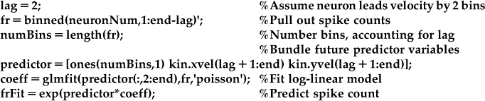
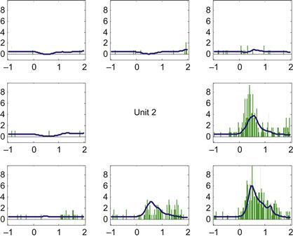
You can now pull out the predicted spike counts centered on the go time, and average them across trials in the same direction to create a predicted PETH. We can then compare this to the empirical PETH we constructed using the code from Chapter 17. If you do this for neuron #2, you should come up with something like Figure 18.4.
18.3 Exercises
1. Implement the log-linear encoding model described in Equation 18.3, and plot the predicted PETH as shown in Figure 18.4. The Moran and Schwartz (1999) paper also included a non-directional speed term. You can access that in the variable kin.speed. Add speed as an extra term to your encoding model. Can you find a neuron where the predicted PETH is better if speed is included? Compare the correlation coefficient between the predicted and actual spike counts across all neurons with and without the speed term. Does adding speed seem to significantly improve the fit across neurons as a population?
2. We assumed a constant lag between neural firing. Instead, try several different lags for each neuron (from +300 ms to −100 ms, in 50 ms steps), and pick the best lag. What is the distribution of best lags across neurons? Compare the correlation coefficient between the predicted and actual spike counts across all neurons with a constant and a variable time lag. Does allowing a variable lag significantly improve the fit across neurons as a population?
18.4 Project
Experiment with alternative encoding models. For example, another paper proposed that neurons encode a movement “pathlet,” meaning that neurons encode velocity at several different time lags with different preferred directions (Hatsopoulos et al., 2007). Is there evidence in this dataset that neurons encode velocity at different time lags? If so, how does the preferred direction change as a function of time?