
Chapter 7
Managing Worksheets and Workbooks

Welcome to this book, designed to help you study for and pass the MO‐200 Microsoft Excel (Excel and Excel 2019) exam and become a certified Microsoft Office Specialist: Excel Associate. If you're all settled in, it's time to get this show on the road.
In this chapter, I'll start by showing you how to import data in other formats into Excel spreadsheets, which Excel calls worksheets, as well as collections of spreadsheets that Excel calls a workbook. Next, I'll show you how to navigate within a workbook and get comfortable with the Excel interface.
When you feel good about creating an Excel spreadsheet, I'll show you how to format that spreadsheet so that it looks the way you want. You'll also learn how to change the way information is presented to make Excel work better for you.
Finally, I'll show you how to get your spreadsheets ready to share in print and online. You'll also learn how to inspect your workbooks so that you can find and remove hidden properties as well as fix any issues with accessibility and compatibility.
I'll have an exercise at the end of every section in this chapter so that you can practice doing different tasks. Then, at the end of this chapter, you'll find a set of Review Questions that mimic the test questions you'll see on the MO‐200 exam.
Importing Data into Workbooks
If you need to import existing data into a workbook, you should first check to see if the file is in a format that Excel likes. The most common formats are the native Excel, text, and comma‐delimited value (CSV) formats.
The native Excel format has the
.xls
filename extension that dates all the way back to MS‐DOS days, so you can obviously open those files. However, if you open an older XLS file, you may experience some issues with formatting.
It is more likely that you will receive files in text format with the
.txt
file extension and in comma‐separated values (CSV) format with the
.csv
file extension. These two formats are what Microsoft focuses on in the MO‐200 exam.
Text and CSV formats use a delimiter, which is a character that separates blocks of text, like between numbers. A text file will use a tab character to separate those blocks. A CSV file uses commas to separate each block of text.
After you open a text file, Excel does not change the format of the file. The file remains with the
.txt
or
.csv
extension as you save updates to it.
Bringing in Data from TXT Files
When you receive a text file from someone else, check the file to ensure that it has a delimiter character. (If you don't see any, then you must decide whether to add the delimiter character or just return the text file to the sender and tell that person to fix the file.)
Once you are satisfied that the text file is ready for Excel, open the text file as follows:
- Click the File menu option.
- Click the Open menu option on the left side of the screen.
- Click Browse.
- In the Open dialog box, click All Excel Files in the lower‐right area of the box.
- Select Text Files from the drop‐down list.
- Navigate to the location that created the text file.
- Click the text filename.
- Click Open.
The Text Import Wizard dialog box opens (see Figure 7.1) and shows you what the text file looks like in step 1 of the wizard. Click the Next button to see what the text will look like in an Excel worksheet, and then click Next again to see the data format Excel assigns to each column.
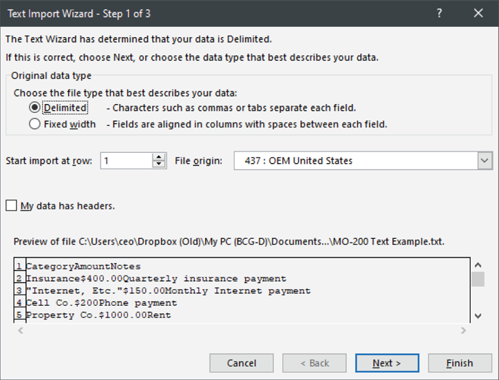
FIGURE 7.1 Text Import Wizard dialog box
Though you can make changes in each of these steps, you don't need to know how to do that for the MO‐200 exam. So, click the Finish button to view the imported spreadsheet.
Import a Text File into an Existing Worksheet
If you have text in another file that you want to place into a new worksheet within a workbook, here's how to do it:
- Click the Data menu option.
- If you see the Need To Import Data pop‐up box, click Got It in the box.
- In the Get & Transform Data section in the Data ribbon, as seen in Figure 7.2, click the From Text/CSV icon.
- In the Import Data dialog box, navigate to the folder that contains the file.
- Select the filename in the list.
- Click Import.
The preview dialog box opens and shows you how the text will appear in the file. Click Load to import the data into a new worksheet with the name Sheet1, as you can see in the list of spreadsheet tabs at the bottom of the Excel window.
Importing Data from CSV Files
A CSV file is formatted specifically to be imported into spreadsheet software, and Excel knows CSV formatting cold. Each cell in a row is on one line of text separated by a comma with no spaces before or after the comma. For example:
Title, Column 1, Column 2
Excel considers each line in a CSV file to be one row, so you may have a CSV file that looks like this:
Date, Payee, Amount, Notes
10/1, InsuranceCo, $400.00, Quarterly insurance payment
A comma does not appear at the end of a line.
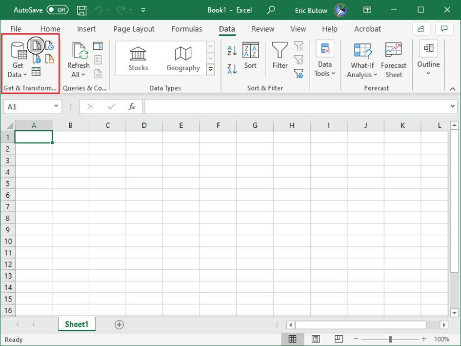
FIGURE 7.2 Get & Transform section
Add a CSV format file by following these steps:
- Click the File menu option.
- Click the Open menu option on the left side of the screen.
- Click Browse.
- In the Open dialog box, click All Excel Files in the lower‐right area of the box.
- Select Text Files from the drop‐down list.
- Navigate to the location that created the text file.
- Click the text filename.
- Click Open.
The Text Import Wizard dialog box opens (see Figure 7.3) and shows you what the text file looks like in step 1 of the wizard. Click the Next button to see what the text will look like in an Excel worksheet, and then click Next again to see the data format that Excel assigns to each column.
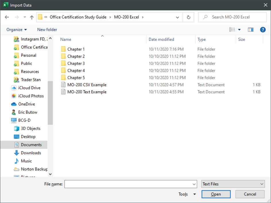
FIGURE 7.3 Import Data dialog box
Insert a CSV File into a New Worksheet
You can also add a CSV file into a new worksheet within a workbook, much as you did with a text file, as follows:
- Click the Data menu option.
- If you see the Need To Import Data pop‐up box, click Got It in the box.
- In the Get & Transform Data section in the Data ribbon (see Figure 7.2), click the From Text/CSV icon.
- In the Import Data dialog box (see Figure 7.3), navigate to the folder that contains the CSV file.
- Click the filename in the list.
- Click Import.
The preview dialog box appears, as shown in Figure 7.4, and it shows you how the text will appear in the file. Click Load to import the data into a new worksheet with the name Sheet1, as you can see in the list of spreadsheet tabs at the bottom of the Excel window.
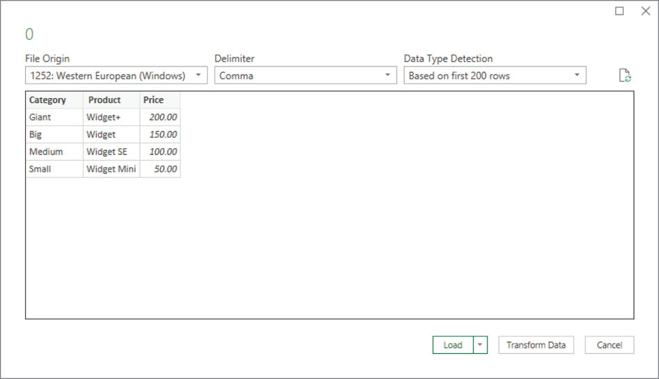
FIGURE 7.4 Preview dialog box
Navigating Within Workbooks
After you populate a workbook, it can seem daunting to try to find the data within it. Excel has tools that make it easy.
Click the Search box in the Excel title bar, and then type the text that you want to find.
Searching for Data Within a Workbook
You can search for data on any worksheet in a workbook by following these steps:
- Click the Home menu option, if necessary.
- In the Editing section in the Home ribbon, click the Find & Select icon.
- Select Find from the drop‐down menu.
The Find And Replace dialog box appears so that you can search for information or replace one or more search terms, including specific formatting, with new text and/or formatting. If you want to replace text, select the Replace tab.
Now you can replace text by typing the text you want to replace in the Find What text box, and then typing the replacement text in the Replace With text box.
Before you find and/or replace text, you may need to specify more information about what you want to find and/or replace. For example, you may want to change not only text in a cell, but also change the font and alignment of that text.
Open all find and replace options by clicking Options in the dialog box. The Find And Replace dialog box expands (see Figure 7.5) so that you can click one of the buttons or boxes to change information, as follows:
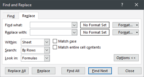
FIGURE 7.5 Find And Replace dialog box
- No Format Set Informs you that no formatting has been applied to the text that you want to find and/or replace. If you change the format, the text in this button changes to Preview so that you can see how the text looks in the worksheet.
- Format Click the button to open the Find Format dialog box and change the format in one of six areas: Number, Alignment, Font, Border, Fill, and Protection. You will learn more about formatting cells later in this chapter.
- Match Case Find text that has the same case as what you typed in the Find box, such as a capitalized first letter in a word.
- Match Entire Cell Contents Find text that appears exactly like what you have typed in the Find box.
- Within The default selection in the Within box is Sheet, which searches for the text in the currently open worksheet. Click Sheet to select from the worksheet or the entire workbook in the drop‐down list.
- Search The default selection in the Search box is By Rows, which searches for all instances of the search text in all rows. If you want to search for all instances of the text in all columns, click By Rows and then click By Columns in the drop‐down list.
- Look In The Look In box has Formulas selected by default, which means that Excel will look for the search term in a specific type of text within the worksheet. If you have the Find tab open, then you can choose from Formulas, Values, Notes, or Comments in the drop‐down list. If you have the Replace tab open, you can only select Formulas.
When you're ready to search for the text that you typed in the Find What text box, click the Find Next button to go to the next instance of the text in the open worksheet. If you search in the entire workbook, Excel searches for the text in the open worksheet first, and then it proceeds to search for all other instances of the text in subsequent worksheets.
If you click Find All, a dialog box appears that lists every instance of the text that Excel found in the worksheet or in the entire workbook. Click the instance in the list to open the cell in the corresponding worksheet.
Click Replace to replace only the next instance of the text with your replacement. If you want to replace any other text that meets your criteria, click the Replace button again to go to the next instance and replace that.
Replace all instances of the text and/or formatting in the Find text box by clicking the Replace All button. When Excel completes its search, a dialog box appears in the middle of the screen and tells you how many changes it made. Close the dialog box by clicking OK.
Navigating to Named Cells, Ranges, or Workbook Elements
Excel allows you to define names for a specific cell or for a range of cells, such as a block of income for a specific month. Here's how:
- Select several cells by clicking and holding on one cell, then dragging the mouse pointer until all cells in the worksheet are highlighted, and then releasing the mouse button.
- Click the Formulas menu option.
- In the Defined Names section in the Formulas ribbon, as shown in Figure 7.6, click Define Name. (If the Excel window width is small, click the Define Name icon in the ribbon and then select Define Name from the drop‐down menu.)
- In the New Name dialog box, press Backspace and then type the new name in the Name box.
- Click OK.
Now that you named a cell, go to another location in your worksheet or another worksheet in the workbook. You can find that named range by following these steps:
- Click the Home menu option, if necessary.
- Click Find And Select in the Editing section in the Home ribbon. (If the Excel window width is small, click the Editing icon in the ribbon and then click the Find And Select icon.)
- From the drop‐down menu, select Go To.
- In the Go To dialog box, shown in Figure 7.7, click the name of the named range.
- Click OK.
Excel highlights the named range within its worksheet.
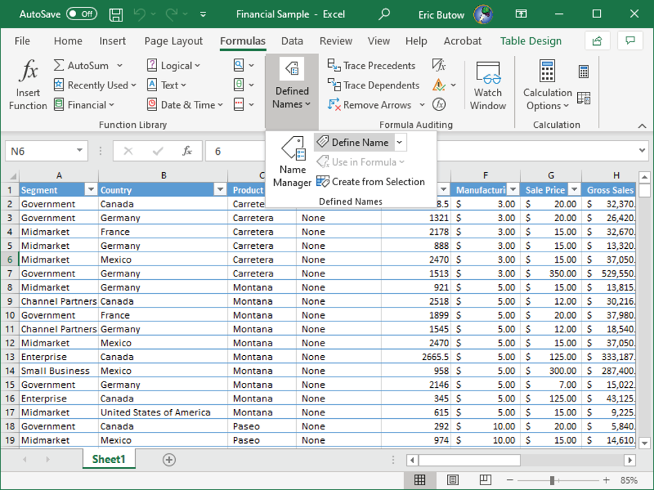
FIGURE 7.6 The Define Name menu option

FIGURE 7.7 Go To dialog box
Inserting and Removing Hyperlinks
You can install as many hyperlinks as you want within the text of your workbook. After you insert a hyperlink, Excel gives you control over copying or moving a hyperlink, changing a hyperlink, and removing a hyperlink.
Start by clicking in the cell where you want to add the hyperlink, and then click the Insert menu option. In the Insert ribbon, click the Link icon, as seen in Figure 7.8. (If the Excel window width is small, click the Links icon in the ribbon and then click the Link icon.)
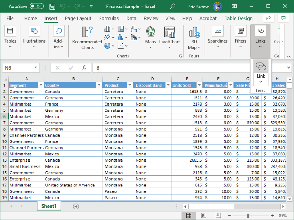
FIGURE 7.8 The Link icon
The Insert Hyperlink dialog box appears (see Figure 7.9) so that you can add your hyperlink.
You can add a hyperlink within the same worksheet, to another worksheet in your workbook, to another file or web page, or to an email address.
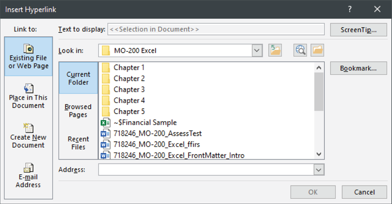
FIGURE 7.9 The Insert Hyperlink dialog box
Within a Workbook
Adding a hyperlink to another location in a worksheet or workbook is useful when you need to move between cells quickly, and especially if you have long worksheets, many worksheets in a workbook, or both.
Start by clicking the cell and then opening the Insert Hyperlink dialog box. In the Link To box on the left side of the dialog box, click Place In This Document, as shown in Figure 7.10.

FIGURE 7.10 The Place In This Document menu option
In the Type The Cell Reference text box, you can type the cell that you want to link to by typing the column letter and then the row number. For example, typing C24 will link to the cell in column C, row 24.
If you want to link to a specific worksheet in your workbook, click the worksheet name under the Cell Reference header in the Or Select A Place In This Document list box.
You can select a named range by scrolling down in the list (if necessary) and then clicking the range name under the Defined Names header.
When you're done, click OK and the hyperlink appears within the text in the cell.
Link to an Existing File
You can add a hyperlink to another file, such as a Word file, that is important to your readers. When you link to another file, the appropriate program, such as Word, opens to view the linked file. Here's how to link to an existing file:
- Click the cell where you want to add the hyperlink.
- Click the Insert menu option.
- In the Link section in the Insert ribbon, click the Link icon that you saw in Figure 7.8. (If the Excel window width is small, click the Links icon in the ribbon and then click the Link icon.)
- In the Link To box on the left side of the dialog box, click Existing File Or Web Page, if necessary.
- Click Current Folder (if necessary) or Recent Files to view the contents in the default Excel folder or all files that you have opened recently, respectively (see Figure 7.11).
- Navigate to the folder that contains the file in the list, if necessary.
- Click the file and then click OK.

FIGURE 7.11 A list of recently opened files
Link to a Web Page
You can add a hyperlink to a web page either on the web or on your network. That web page can be the home page, in which case you only need to type the URL of the site. If you need to link to a specific web page, you must type the full URL, including the web page name. You can also view recently browsed pages and select the page from the list.
When you link to a website, the default web browser opens and displays the page (or an error if the link is incorrect). Here's how to link to a web page:
- Click the cell where you want to add the hyperlink.
- Click the Insert menu option.
- In the Link section in the Insert ribbon, click the Link icon that you saw in Figure 7.8. (If the Excel window width is small, click the Links icon in the ribbon and then click the Link icon.)
- In the Link To box on the left side of the dialog box, click Existing File Or Web Page, if necessary.
- Click Browsed Pages to view a list of all the web pages (see Figure 7.12).
- Scroll up and down the list (if necessary), click the web page that you want to open, and then proceed to step 8.
- If you don't see the web page that you want in the list, type the full URL in the Address box. That is, type
http://orhttps://before the website and any specific web pages. - Click OK.

FIGURE 7.12 Browsed Pages list
The link appears in the cell, and you can click the link to see if it opens the web page.
To an Email Address
Excel allows you to open a new email message so that you can send a message to that email address. You can also add a subject to the message. When you click the link, the default email program opens a new message window so that you can begin typing your message to the recipient.
Link to an email address by following these steps:
- Click the cell where you want to add the hyperlink.
- Click the Insert menu option.
- In the Link section in the Insert ribbon, click the Link icon that you saw in Figure 7.8. (If the Excel window width is small, click the Links icon in the ribbon and then click the Link icon.)
- In the Link To box on the left side of the Insert Hyperlink dialog box (see Figure 7.13), click E‐mail Address.
- Type the email address in the E‐mail Address text box.
- Add a subject for your message in the Subject text box.
- Click OK.

FIGURE 7.13 E‐mail Address menu option
Copy and Move a Hyperlink
Once you create a hyperlink, you can copy it or move it to another cell. Here's how to do this:
- Click the cell with the link that you want to move.
- Click the Home menu option, if necessary.
- Copy the cell with the link by clicking the Copy icon in the Clipboard section in the Home ribbon, and then proceed to step 5.
- Move the cell with the link by clicking the Cut icon in the Clipboard section in the Home ribbon.
- Click the cell in the workbook where you want to paste the text with the link.
- Click the Paste icon in the Clipboard section in the Home ribbon.
Change a Hyperlink
Excel allows you to change a hyperlink in a cell in one of three ways:
- You can change the destination of the link.
- You can change how the link appears in the cell.
- You can change the text in the cell and keep the link intact.
Start by clicking on a location in the cell that is outside the text with the link. If you can't, then click an adjacent cell and then use the arrow keys on your keyboard to highlight the cell with the hyperlink. (You will learn to change column widths and row height later in this chapter.)
Now you can open the Edit Hyperlink dialog box the same way you did when you inserted a hyperlink. The Edit Hyperlink dialog box appears (see Figure 7.14) and shows you the details of your hyperlink.
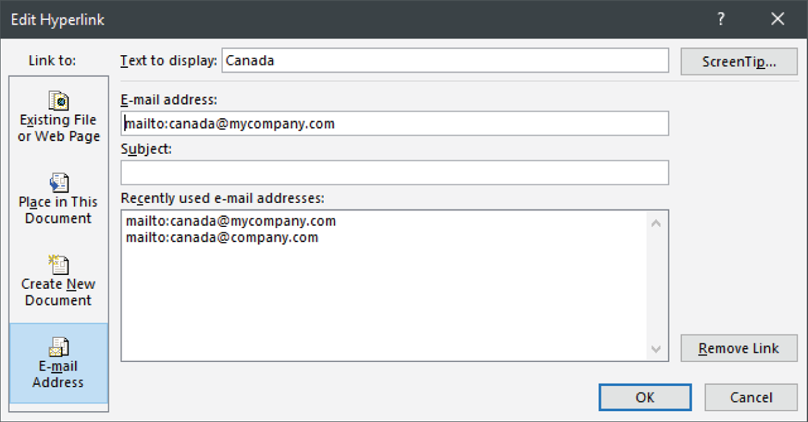
FIGURE 7.14 Edit Hyperlink dialog box
For example, if you link to an email address, then the E‐mail Address option is selected in the Link To box, and you can see the email address and subject (if there is one) so that you can update that information quickly.
If you need to change the linked text that appears in the hyperlink, you can do so in the Text To Display box at the top of the dialog box.
When you finish making your changes, click OK. If you changed the link destination or email address, you may want to click the link to make sure that it works the way you expect.
You can change an existing hyperlink in your workbook by changing its destination, its appearance, or the text or graphic that is used to represent it.
Delete a Hyperlink
If you need to delete hyperlinked text in a cell, all you have to do is right‐click the cell that has the link. In the context menu, as seen in Figure 7.15, click Remove Hyperlink. The link disappears from the text.

FIGURE 7.15 The Remove Hyperlink option in the context menu
You can also delete the text in the cell as well as the link by right‐clicking on the cell and then clicking Clear Contents in the context menu.
Formatting Worksheets and Workbooks
As you work with Excel, you may want to format how worksheets in a workbook appear, perhaps because you want it to look that way, people with whom you share the workbook expect it to look a certain way, or both. Excel allows you to modify the page settings, adjust the height of rows and the width of columns, and add headers and footers to pages, much as you would in a Word document.
Modifying Page Settings
When you need to modify page settings, begin by clicking the Page Layout menu option. The Page Setup section in the Page Layout ribbon (see Figure 7.16) shows you all the tools that you can use to change the page settings.

FIGURE 7.16 Page Setup section options
All of these icons appear in the ribbon no matter whether your window width is 800 pixels, as seen in Figure 7.16, or larger. Click one of the following options to make changes:
- Margins Change the margins for each printed page within a worksheet in the drop‐down menu. The default is Normal, but you can select from Wide and Narrow margins. If none of the default options work for you, click Custom Margins at the bottom of the menu and then set your own margins in the Page Setup dialog box.
- Orientation Change between Portrait and Landscape orientation in the drop‐down menu. The default is Portrait.
- Size Set the paper size in the drop‐down menu. The default is Letter, which is 8.5 inches wide by 11 inches high. If none of the paper sizes meet your needs, click More Page Sizes at the bottom of the menu and then set your own paper size in the Page Setup dialog box.
- Print Area If you want to print a range of cells within a worksheet, select the cells by clicking and holding one cell in the range and then dragging until Excel selects all the cells. When you're done, release the mouse button and then click Print Area. From the drop‐down list, select Set Print Area. You can remove the print area by clicking Print Area and then selecting Clear Print Area from the drop‐down menu. You will learn more about setting a print area later in this chapter.
- Breaks Add a page break after the currently selected cell or row in your worksheet by selecting Insert Page Break from the drop‐down menu. You can also remove the page break after the currently selected cell by clicking Remove Page Break. If you want to remove all page breaks in the workbook, click Reset All Page Breaks.
- Background Add a background image to your worksheet. You can add an image from a file on your computer, from the web using a Bing search, or from a OneDrive folder.
- Print Titles Opens the Page Setup dialog box so that you can tell Excel to print the same rows at the top and/or same columns at the left side of your printed worksheet.
Adjusting Row Height and Column Width
Excel has default row heights and column widths, but you may have to change those for readability. For example, you may need to extend the column width so that you can see all of the text in a cell within that column. The minimum, default, and maximum heights for rows and columns are as follows:
- Minimum height, rows, and columns: 0 points
- Default row height: 15 points
- Default column width: 8.43 points
- Maximum row height: 409 points
- Maximum column width: 255 points
Set Column to Specific Width
Here's how to change the column width:
- Select a cell in the column.
- Click the Home menu option, if necessary.
- In the Cells section in the Home ribbon, click the Format icon. If your Excel window width is smaller, as shown in Figure 7.17, click the Cells icon and then click the Format icon.
- Select Column Width from the drop‐down menu, as shown in Figure 7.17.
- In the Column Width dialog box, press the Backspace key to delete the highlighted measurement.
- Type the new width in points.
- Click OK.

FIGURE 7.17 Column Width option
Change the Column Width to Fit the Contents Automatically with AutoFit
Excel has a built‐in AutoFit feature that allows you to fit the width of the contents automatically. AutoFit a column by following these steps:
- Select a cell in the column.
- Click the Home menu option, if necessary.
- In the Cells section in the Home ribbon, click the Format icon. If your Excel window width is smaller, as shown in Figure 7.18, click the Cells icon and then click the Format icon.
- Select AutoFit Column Width from the drop‐down menu, as shown in Figure 7.18.

FIGURE 7.18 AutoFit Column Width option
The column width changes to accommodate the text in the cell with the longest width.
Match the Column Width to Another Column
If you want more than one column to have the same width, here's how to do that:
- Click a cell within the column that has your preferred width.
- Click the Home menu option, if necessary.
- In the Clipboard section in the Home ribbon, click Copy.
- Click a cell in the column to which you want to apply the width.
- In the Clipboard section in the Home ribbon, click the down arrow under the Paste icon.
- Click the Keep Source Column Widths icon in the drop‐down menu, as shown in Figure 7.19.
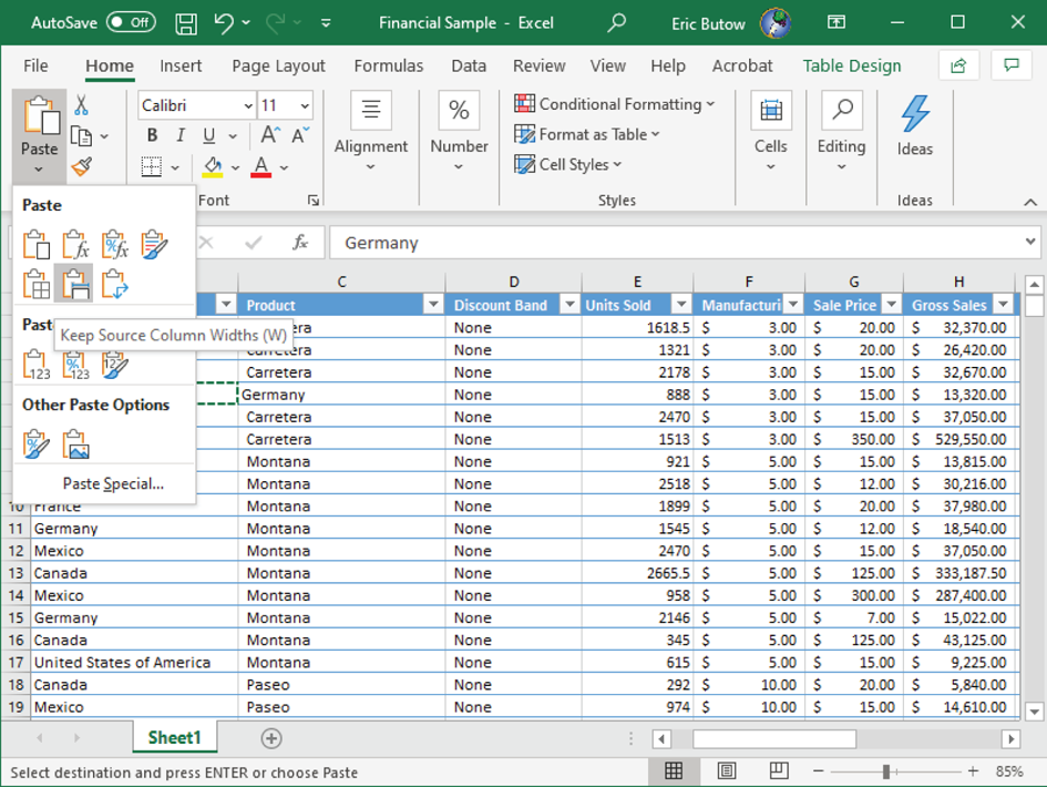
FIGURE 7.19 Keep Source Column Widths icon
When you move the mouse pointer over the icon, the column width changes automatically so that you can preview the width of the column before you click the icon. If you move the mouse pointer away from the icon, the column reverts to its previous width.
Change the Default Width for All Columns on a Worksheet
If all you need is one width for all columns within a worksheet, change the default width by following these steps:
- Click the Home menu option, if necessary.
- In the Cells section in the Home ribbon, click Format. If the width of your Excel window is smaller, click the Cells icon and then click Format.
- Select Default Width from the drop‐down menu, as shown in Figure 7.20.
- In the Standard Width dialog box, press Backspace to delete the width in the Standard Column Width text box.
- Type the new width in points.
- Click OK.

FIGURE 7.20 Default Width option
Excel resizes all columns in the worksheet to the width you specified.
Change the Width of Columns by Using the Mouse
When you want to change the width of a column by using the mouse, move the mouse pointer to the right border of the column heading above the worksheet. The cursor changes to a double‐headed arrow, as shown in Figure 7.21.

FIGURE 7.21 The resize mouse pointer between two column headings
Now you can click, hold, and drag the boundary of the column heading to the left or right. As you drag, the width of the column to the left of the pointer changes, and a pop‐up box above the pointer shows you the exact width of the column. When the column is the size that you want, release the mouse button.
Set a Row to a Specific Height
When you want to set a row to a specific height, the process for doing so is much the same as setting a column to a specific width, as follows:
- Select a cell in the row.
- Click the Home menu option, if necessary.
- In the Cells section in the Home ribbon, click the Format icon. If your Excel window width is smaller, as shown in Figure 7.22, click the Cells icon and then click the Format icon.
- Select Row Height from the drop‐down menu, as shown in Figure 7.22.
- In the Row Height dialog box, press the Backspace key to delete the highlighted measurement.
- Type the new height in points.
- Click OK.
Excel resizes the row and vertically aligns the text at the bottom of the cells in the row.
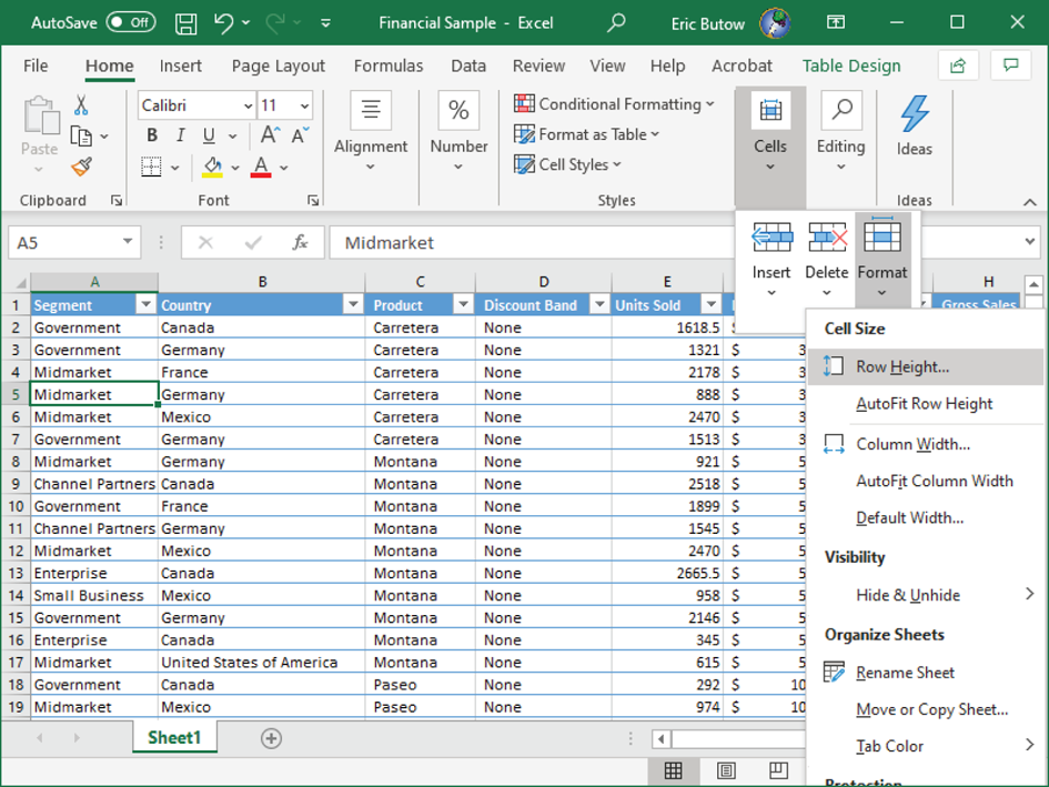
FIGURE 7.22 Row Height option
Change the Row Height to Fit the Contents with AutoFit
As with columns, the built‐in AutoFit feature allows you to fit the height of rows automatically to match the largest height in a row. Here's how to do this:
- Select a cell in the row.
- Click the Home menu option, if necessary.
- In the Cells section in the Home ribbon, click the Format icon. If your Excel window width is smaller, as shown in Figure 7.23, click the Cells icon and then click the Format icon.
- Select AutoFit Row Height from the drop‐down menu, as shown in Figure 7.23.
The row height changes to accommodate the text in the cell with the largest height.
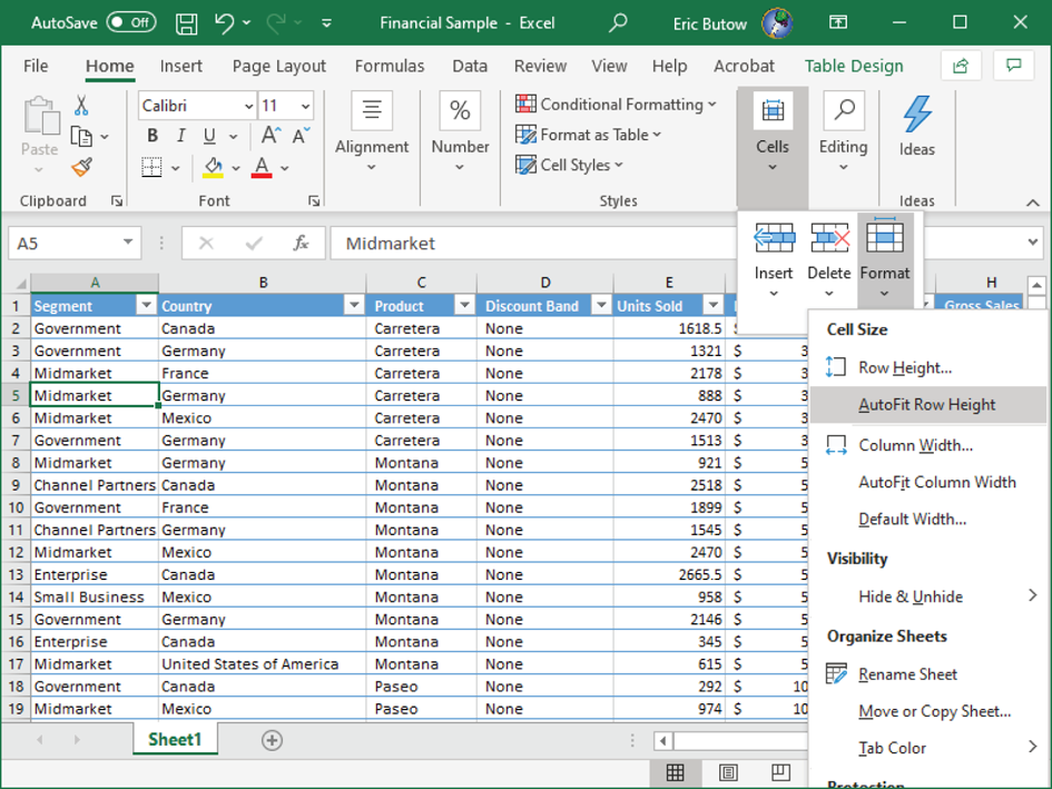
FIGURE 7.23 AutoFit Row Height option
Change the Height of Rows by Using the Mouse
You can change the height of a row more quickly by using the mouse. Start by moving the mouse pointer to the bottom border of the row heading to the left of the worksheet. The cursor changes to a double‐headed arrow, as shown in Figure 7.24.

FIGURE 7.24 The resize mouse pointer between two row headings
Now you can click, hold, and drag the boundary of the row heading up and down. As you drag, the height of the row above the pointer changes, and a pop‐up box above the pointer shows you the exact height of the row. When the row is the size that you want, release the mouse button.
Customizing Headers and Footers
As with a Word document, you can add headers and footers into an Excel spreadsheet that will make it easier for users who view your documents in paper or PDF format to read it. For example, a header can include the title of the document and the footer can include a page number. Excel also makes it easy to customize headers and footers.
Add a Header or Footer
Add a header and footer into a worksheet by clicking the Insert menu option. In the Text section in the Insert menu ribbon, click the Header & Footer icon in the Text section (see Figure 7.25).

FIGURE 7.25 Header & Footer icon
The worksheet appears in Page Layout view with the cursor blinking within the middle section of the header. The cursor is in the center position so that the text will be centered on the page.
Click the left section of the header to place the cursor so that it is left‐aligned in that section. Click the right section of the header to place the cursor right‐aligned in that header. The text in all three sections in the header are vertically aligned at the top.
The Header & Footer ribbon appears automatically so that you can add a footer by clicking the Go To Footer icon in the Navigation section. The footer section appears at the bottom of the spreadsheet page with the cursor blinking in the center section of the footer.
Like the Header section, the footer is divided into three sections, but the text in all three sections is vertically aligned at the bottom. You can return to the header by clicking the Go To Header icon in the ribbon.
Add Built‐In Header and Footer Elements
Excel contains a number (ahem) of features for adding header and footer elements so that you don't have to update them automatically, such as with a page number.
After you add a header or footer and you have clicked within a section, the Header & Footer ribbon appears. You can add built‐in elements from the Header & Footer and the Header & Footer Elements sections.
Header & Footer Section
In the Header & Footer section in the ribbon, click the Header icon to view a list of built‐in header elements that you can add (see Figure 7.26).
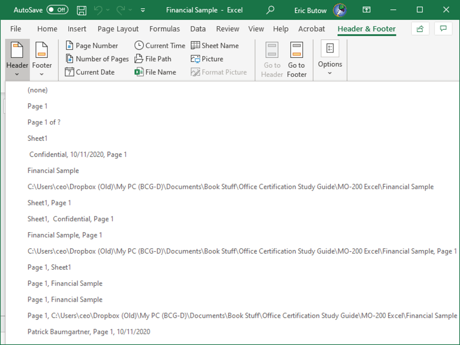
FIGURE 7.26 Header element drop‐down list
Some entries in the list have two or three options. An entry with two elements will place them in the header sections specified within the built‐in entry. For example, the page number appears in the center section and the worksheet name appears in the right section.
After you select a header element from the drop‐down list, Excel adds the header automatically and places the cursor back in the worksheet so that you can resume your work.
If you click within a footer, you can add a built‐in footer element by clicking the Footer icon and then selecting a built‐in footer element from the drop‐down list. Once you do, Excel adds the footer and places the cursor in the worksheet.
Header & Footer Elements
The Header & Footer Elements section contains nine elements, as shown in Figure 7.27.
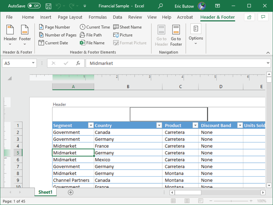
FIGURE 7.27 Header & Footer Elements section
When you click one of the buttons (except for Format Picture, which is only active after you add a picture), its field name appears within brackets and preceded by an ampersand (
&
), such as
&[Date]
. Some fields are preceded by text, such as
Page &[Page]
.
After you add the element and click outside the header or footer, the element appears properly. Click one of the icons in the ribbon to add the element.
- Page Number Adds the current page number in the worksheet
- Number Of Pages Displays the number of pages in the worksheet that contain data
- Current Date Displays the current date. Excel does not update the date until you click the date in the header or footer and then click in the worksheet again.
- Current Time Displays the current time. Excel updates the time when you click the time in the header or footer and then click in the worksheet.
- Add the workbook folder path and file name Add a page break after the currently selected cell or row in your worksheet by selecting Insert Page Break from the drop‐down menu. You can also remove the page break after the currently selected cell by clicking Remove Page Break. If you want to remove all page breaks in the workbook, click Reset All Page Breaks.
- Add the workbook file name Add a background image to your worksheet. You can add an image from a file on your computer, from the web using a Bing search, or from a OneDrive folder.
- Add the worksheet name Opens the Page Setup dialog box so that you can tell Excel to print the same rows at the top and/or the same columns at the left side of your printed worksheet
- Picture Opens the Insert Pictures dialog box so that you can insert a picture from a file on your computer or network, from a Bing Image Search, or from your default OneDrive folder. If the picture is larger than the header or footer, the picture appears on the page within the left and right margins.
- Format Picture Opens the Format Picture dialog box so that you can change the size and orientation, crop the picture, change the color, brightness, and contrast settings, and add alternative (Alt) text
Delete a Header and Footer
If you need to delete the element, double‐click the element name to select it, and then press Delete on the keyboard. The header and footer remain in the document, and the page separator dashes appear in the worksheet.
You can delete the header and footer from the entire workbook by following these steps:
- Click the Page Layout menu option.
- In the Page Setup section in the Page Layout ribbon, click Print Titles.
- In the Page Setup dialog box, as shown in Figure 7.28, click the Header/Footer tab.
- Click the header and/or footer name in the Header or Footer box, respectively.
- Click (none) in the list. (You may need to scroll up and down in the list to find it.)
- Click OK.

FIGURE 7.28 Page Setup dialog box
Customizing Options and Views
Excel offers you plenty of ways to change the options that you can access as you work in a workbook, as well as what you see in ribbons and toolbars so that you can get your work done more quickly.
You can customize the Quick Access Toolbar, create and modify custom views, and freeze rows and columns in a worksheet so that they don't move as you navigate within a worksheet.
Customizing the Quick Access Toolbar
Excel includes a toolbar for accessing tools and commands quickly without having to click the menu option and then find the option in the ribbon. Microsoft naturally calls this the Quick Access Toolbar, and you can add features from a ribbon to the toolbar.
The toolbar itself appears at the left side of the Excel window title bar, but you can move the toolbar below the ribbon instead. By default, there are only four commands that you can access in the toolbar:
- You can turn the AutoSave feature off and on; the default setting is off.
- Save
- Undo
- Redo
Add a Command to the Quick Access Toolbar
You can add a command to the toolbar in one of two ways. The first is to add the command from a ribbon. The other is to add a command from the Customize Quick Access Toolbar menu.
Add from the Ribbon
Whenever you're in a ribbon and you see an option that you want to add to the Quick Access Toolbar, here's what to do:
- Click the menu option to open its associated ribbon.
- In the ribbon, right‐click the word or icon associated with the command that you want to add to the toolbar.
- Select Add To Quick Access Toolbar from the drop‐down menu (see Figure 7.29).
You see the new icon at the right side of the toolbar, as you can also see in Figure 7.29.
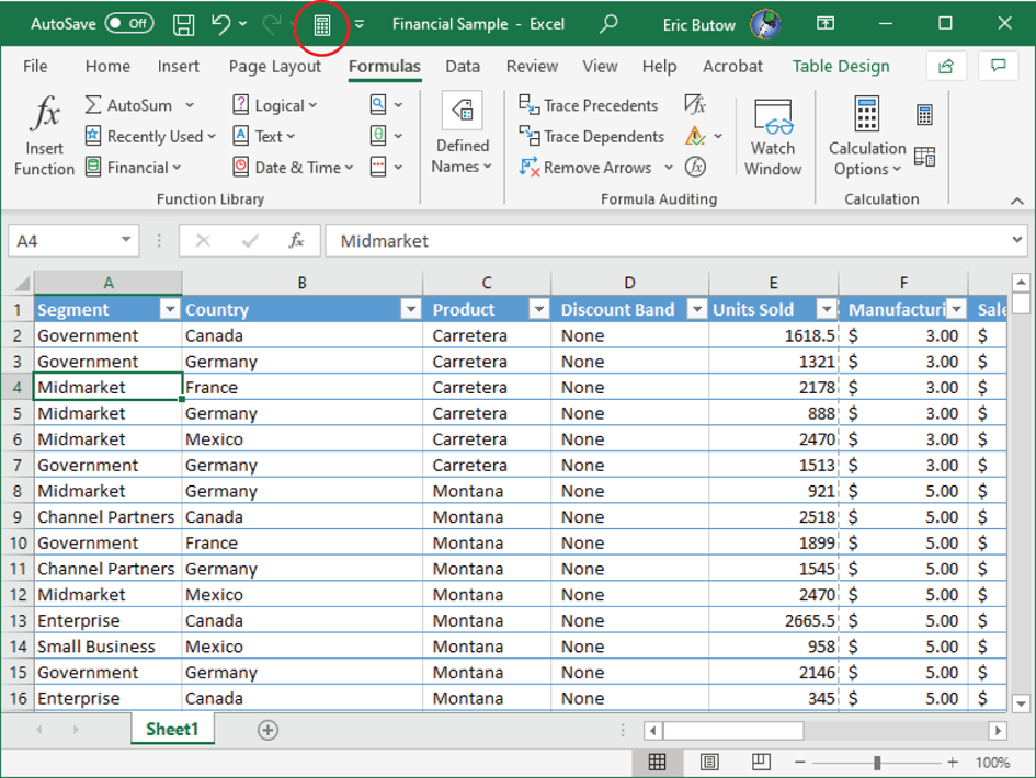
FIGURE 7.29 The new icon in the Quick Access Toolbar
Add from the Customize Quick Access Toolbar Menu
You can also add a command from the Customize Quick Access Toolbar drop‐down menu. Start by clicking the down arrow at the right side of the Quick Access Toolbar in the Excel window title bar. If you haven't added any icons to the toolbar, you will see the icon to the right of the Redo icon.
Next, click one of the options without a check mark to the left of the command name in the drop‐down menu, as you can see in Figure 7.30. (You will learn how to remove options from the toolbar later in this chapter.)

FIGURE 7.30 Customize Quick Access Toolbar drop‐down menu
Remove a Command from the Quick Access Toolbar
There are two ways that you can remove a command from the Quick Access Toolbar:
- Right‐click the command in the toolbar, and then select Remove From Quick Access Toolbar from the drop‐down menu.
- Click the down arrow at the right side of the Quick Access Toolbar, and then click a command that has a check mark next to it.
In both cases, the icon disappears from the toolbar and you can go back to work.
Move the Quick Access Toolbar
By default, the Quick Access Toolbar appears within the Excel window title bar. You can move the toolbar below the ribbon, where it will stay even if you close Excel and reopen it.
All you need to do to move the Quick Access Toolbar is click the down arrow at the right side of the toolbar and then click Show Below The Ribbon. The toolbar appears under the ribbon (see Figure 7.31).

FIGURE 7.31 The Quick Access Toolbar below the ribbon
If you want to move the toolbar back, click the down arrow at the right side of the toolbar and then select Show Above The Ribbon from the drop‐down menu.
Reset the Quick Access Toolbar to the Default Settings
Follow these steps if you need to reset the Quick Access Toolbar to its default settings:
- Click the down arrow at the right side of the Quick Access Toolbar.
- Select More Commands from the drop‐down menu.
- Click Reset in the Excel Options dialog box, as shown in Figure 7.32.
- Select Reset Only Quick Access Toolbar from the drop‐down menu.
- Click Yes in the Reset Customizations dialog box.
- Click OK.
All of the commands that you added in the toolbar disappear, and you see only the four default options.

FIGURE 7.32 Reset button in Excel Options dialog box
Displaying and Modifying Workbook Content in Different Views
Excel allows you to change the view on the document so that you can zoom in and zoom out within a worksheet, but Excel only has five built‐in magnification levels, from 25 percent to 200 percent, as well as the ability to fit the worksheet to the window.
What's more, you can set your own custom view type. Here's how:
- Click the View menu option.
- In the Zoom section in the View ribbon, click the Zoom icon.
- In the Zoom dialog box, as shown in Figure 7.33, select the custom view or type it in the Custom box. The default custom setting is 100 percent.
- Click OK.

FIGURE 7.33 Zoom dialog box
When you view your document, Excel allows you to create a custom view to make workbook content appear the way you prefer. You can save three different types of views:
- Display settings: Used to hide rows, columns, and filter settings
- Print settings: Used to set margins, headers, footers, and other worksheet and page settings
- A specific print area: Settings applied to a particular print area
You can also create multiple views, each with a different name.
Create a Custom View
Here's how to create a custom view in a worksheet:
- Click the View menu option.
- In the Workbook Views section in the View ribbon, click the Custom Views icon (see Figure 7.34).
- In the Custom Views dialog box, click Add.
- In the Add View dialog box, as shown in Figure 7.35, type the name for the view in the Name box.
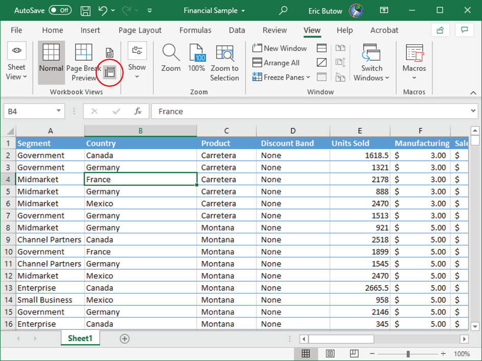
FIGURE 7.34 Custom Views icon
- The two view settings are selected by default so that you will view print settings as well as hidden row, column, and filter settings. Turn one or both views off by clicking the appropriate check box.
- Click OK.
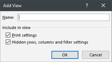
FIGURE 7.35 Add View dialog box
Apply a Custom View
When you want to show a view, open the Custom Views dialog box again. You see the view highlighted in the list, as seen in Figure 7.36. (If you have more views than the window can hold, scroll up and down in the list to find it.) Click the view name in the list, if necessary, and then click Show.

FIGURE 7.36 The selected view in the list is at the top.
You see the changes in your view. For example, if your custom view is 150 percent, the view of your worksheet changes to 150 percent of the default magnification.
Delete a Custom View
When you want to delete a custom view, follow these steps:
- Open the Custom Views dialog box, as you learned to do earlier in this chapter.
- In the Custom Views dialog box, click the view that you want to delete in the list.
- Click Delete.
- Click Yes in the dialog box.
The view disappears from the list. Close the dialog box by clicking Close.
Freezing Worksheet Rows and Columns
You can freeze a row or column in a worksheet so that a row and/or column remains visible on the worksheet even as you scroll through it. This feature is especially useful if you have header rows or columns to which you will need to refer as you scroll through a worksheet that doesn't fit in the Excel window.
Freeze the First Column
If you only want to freeze the first column in the worksheet (that is, column A), follow these steps:
- Click the View menu option.
- In the Window section, click Freeze Panes.
- Select Freeze First Column from the drop‐down menu, as shown in Figure 7.37.
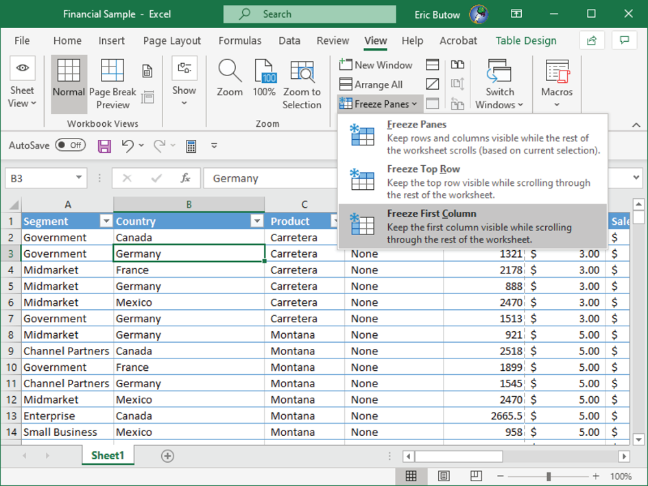
FIGURE 7.37 Freeze Panes drop‐down menu
A darker line appears at the right edge of column A, which shows you that the column is frozen.
Freeze the First Row
If you want to freeze only the first row in the worksheet (that is, row 1), follow these steps:
- Click the View menu option.
- In the Window section in the View ribbon, click Freeze Panes.
- Select Freeze Top Row from the drop‐down menu in Figure 7.37.
A darker line appears at the right edge of row 1, which shows you that the row is frozen.
Freeze Any Column or Row
You can select one or more columns or rows to freeze. However, you need to select the cell below the row(s) and to the right of the column(s) that you want to freeze. After you do that, follow these steps:
- Click the View menu option.
- In the Window section, click Freeze Panes.
- Select Freeze Panes from the drop‐down menu in Figure 7.37.
The line above the selected cell and the line to the left of the selected cell are darker. This means that all rows above the darker line and all columns to the left of the darker line are frozen.
Unfreeze Rows and Columns
If you decide that you no longer want a row and/or column frozen, here is how to unfreeze all rows and columns:
- Click the View menu option.
- In the Window section in the View ribbon, click Freeze Panes.
- Select Unfreeze Panes from the drop‐down menu.
You only see the Unfreeze Panes option if you have one or more frozen rows and/or columns.
Changing Window Views
By default, Excel shows the worksheet in what it calls Normal view, which shows the worksheet. When you need to view the worksheet before you print it to your printer or to a PDF file, you can view where the page breaks are on each page in the Page Break Preview view, as well as how the worksheet will appear on each page in the Page Layout view.
Page Break Preview
View all the page breaks in your worksheet by first clicking the View menu option. Then, in the View ribbon, click the Page Break Preview icon in the Workbook Views section. The worksheet appears with page breaks, as shown in Figure 7.38.
Pages are bordered by a solid blue line. Page breaks are denoted by a dashed blue line. As you scroll up and down the pages, you see gray page numbers in the background, but Excel does not print these page numbers.
Page Layout View
If you need to see how a worksheet appears on printed pages, as well as add a header and/or footer, you need to view your worksheet in Page Layout view.

FIGURE 7.38 Page Break Preview view
Start by clicking the View menu option. In the View ribbon, click the Page Layout View icon. You see the worksheet contained within graphic representations of pages along with a ruler above and to the left of each page (see Figure 7.39).
Click Add Header at the top of the page and click Add Footer at the bottom of the page to add a header and footer, respectively.
Normal View
If you're viewing the worksheet in Page Break Preview view or Page Layout view, you can return to Normal view by first clicking the View menu option. Then, in the View ribbon, click the Normal icon in the Workbook Views section.
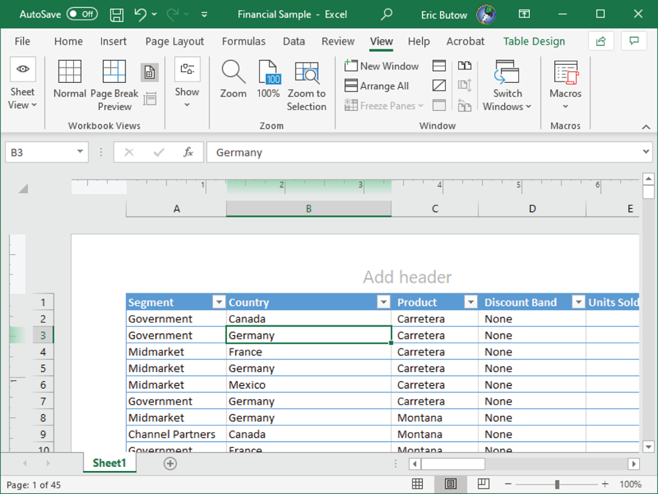
FIGURE 7.39 Page Layout view
Modifying Basic Workbook Properties
Excel constantly keeps track of basic properties about your workbook, including the size of the workbook file, who last edited it, and when the workbook was last saved.
If you need to see these properties and add some of your own, click the File menu option. In the menu on the left side of the File screen, click Info. Now you see the Info screen, which is shown in Figure 7.40.
The Properties section appears at the right side of the screen. Scroll up and down in the Info screen to view more properties. Excel doesn't show all properties by default, but you can reveal the hidden properties by clicking the Show All Properties link at the bottom of the Properties section.
You can also add properties, including a workbook title, a tag (which is Microsoft's term for a keyword), and a category. For example, click Add A Title in the Properties section to type the workbook title in the box.
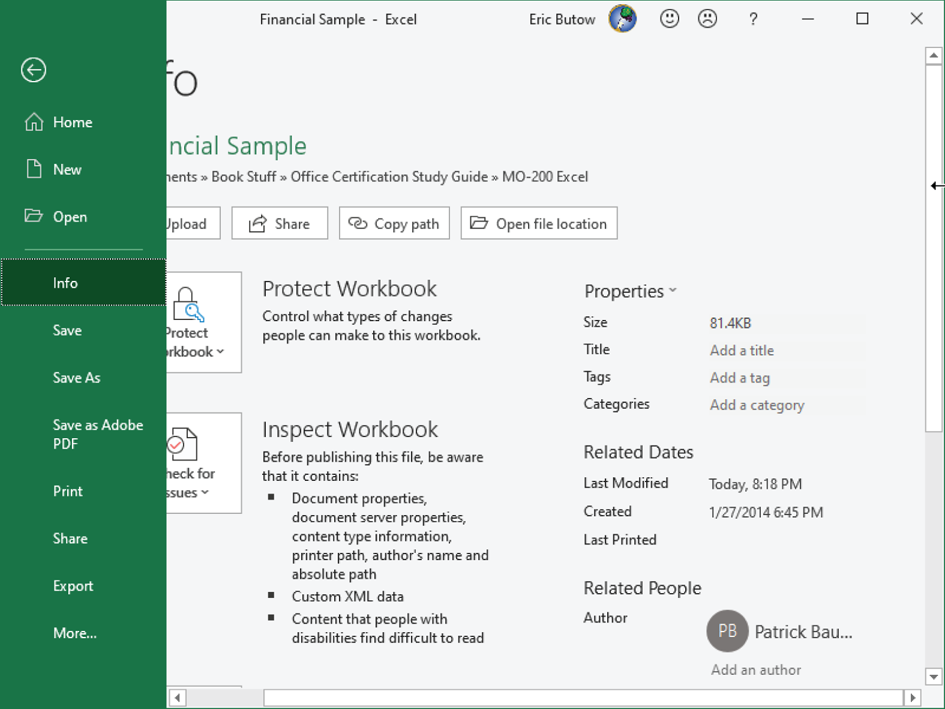
FIGURE 7.40 Info screen
Displaying Formulas
Excel gives you ways to display and hide formulas, as well as their results, from within a workbook. You can also protect the worksheet to keep your views from being changed by anyone with whom you share your workbook.
Switch Between Displaying Formulas and Their Results
By default, Excel shows the results of a formula within the worksheet but only shows the formula in the Formula Bar above the worksheet.
You can display the formula by pressing Ctrl+`. The grave (
`
) accent is on the key with the tilde (
~
) on most keyboards. You can hide the formula again by pressing Ctrl+`.
When you show the formula in the worksheet, the width of the column changes to accommodate as much of the formula as possible. When you show the result again, Excel returns the column width to where it was before you displayed the formula.
Hide a Formula in the Formula Bar
You can hide a formula in the Formula Bar, but only if the worksheet is protected. After you click the cell or select a range of cells with formulas you want to hide, follow these steps:
- Click the Home menu option, if necessary.
- In the Cells section in the Home ribbon, click Format. (If the Excel window width is small, click the Cells icon in the ribbon and then select Format from the drop‐down menu.)
- Select Format Cells from the drop‐down menu.
- In the Format Cells drop‐down menu, select Protect Sheet, as shown in Figure 7.41.

FIGURE 7.41 Protect Sheet option
- Click the Hidden check box.
- Click OK.
- Click the Review menu option.
- In the Protect section in the Review ribbon, click Protect Sheet (see Figure 7.42). (If the Excel window width is small, click the Protect icon in the ribbon and then select Protect Sheet from the drop‐down menu.)
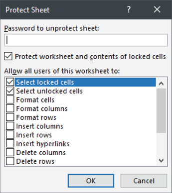
FIGURE 7.42 Protect Sheet dialog box
- In the Protect Sheet dialog box, leave all the check boxes selected. You can add a password in the Password To Unprotect Sheet text box if you plan to share the workbook with anyone else. Otherwise, click OK.
The formula no longer appears in the Formula Bar.
Configuring Content for Collaboration
Excel makes it easy to share workbooks with other people, such as people in the finance, sales, and marketing departments who need to see financial forecasts for the next quarter. Before you do that, you must determine what information you want to share.
You can set a print area within a worksheet, save your workbook in a different format, configure your print settings before you print a document to share on paper or electronically, and inspect your workbook so that you can hide information that you want to keep hidden.
Setting a Print Area
If you print a specific area of rows and columns often, such as a summary of the company's profit and loss for the current quarter, Excel allows you to define a print area within a worksheet.
After you select the cells that you want in the print area within the worksheet, set the print area as follows:
- Click the Page Layout menu option.
- In the Page Setup section in the Page Layout ribbon, click Print Area.
- Click Set Print Area, as shown in Figure 7.43.
- Click outside the selected area in the worksheet to view the print area, which has a dark gray border around the cell or group of cells in the print area.
Excel saves the print area after you save the workbook.

FIGURE 7.43 Set Print Area option
Saving Workbooks in Other File Formats
Microsoft realizes that you may need to save Excel workbooks in different formats to share them with other people who may have older versions of Excel, other spreadsheet apps (like Google Sheets), or no spreadsheet program at all. Rest easy—Excel has you covered.
Here's how to save a workbook in a different file format:
- Click the File menu option.
- Click Save As in the menu on the left side of the File screen.
- On the right side of the Save As screen, click the Excel Workbook (
*.xlsx) box. - Select one of the file formats from the list shown in Figure 7.44. These formats come from a variety of categories, including older versions of Excel, CSV, HTML, XML, PDF, and text.
- Click Save.
Excel saves a copy of the worksheet in the directory where you have the Excel worksheet. Your Excel worksheet remains active so that you can continue to work on it if you want.
Configuring Print Settings
Before you print to either a printed page or to PDF format, you can view the print preview settings and make changes in Excel.
Excel easily detects the default printer that you're using in Windows and lets you change the printer settings so that your document appears on paper the way you want.
Start by clicking the File menu option, and then click Print in the menu on the left side of the File screen. Now you see the Print screen, and the print preview area appears on the right side so that you have a good idea of what the worksheet will look like on the printed page.
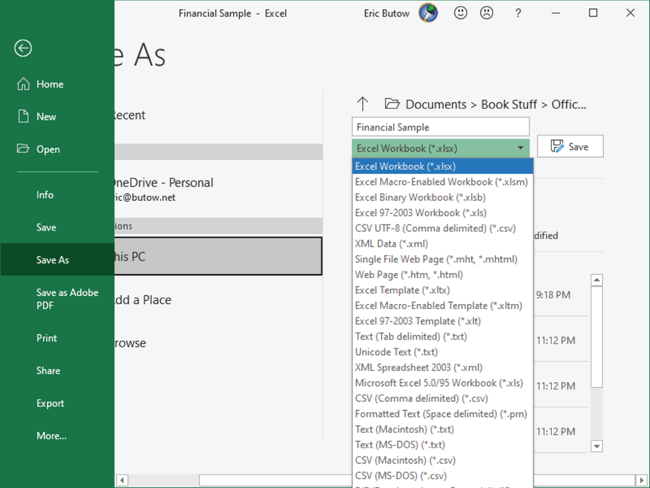
FIGURE 7.44 A partial list of file formats
Between the menu area on the left and the print preview area, the Settings menu you see depends on the printer you have.
In my case, I can change the printer to another one that I have installed in Windows, as shown in Figure 7.45. I can also change different settings for the selected printer, including how many pages to print, the page orientation, and whether I should print on one or both sides of the paper.
Inspecting Workbooks for Issues
Before you share a workbook with other people, such as in an email attachment, you should take advantage of the Document Inspector in Excel to find information that you may not realize is saved with your workbook. For example, Excel saves author information, and you may not want to share that information when you share the workbook with someone outside your company.

FIGURE 7.45 Print screen
Start by clicking the File menu option. Click Info in the menu bar on the left side of the File screen. Now that you're in the Info screen, click the Check For Issues button. From the drop‐down list, select Inspect Document.
Now you see the Document Inspector dialog box, as shown in Figure 7.46. Scroll up and down the list of content that Windows will inspect.
By default, the following check boxes next to the content category names are selected:
- Comments
- Document Properties And Personal Information
- Data Model
- Content Add‐Ins

FIGURE 7.46 Document Inspector dialog box
- Task Pane Add‐Ins
- PivotTables, PivotCharts, Cube Formulas, Slicers, and Timelines
- Embedded Documents
- Macros, Forms, And ActiveX Controls
- Links To Other Files
- Real Time Data Functions
- Excel Surveys
- Defined Scenarios
- Active Filters
- Custom Worksheet Properties
- Hidden Names
- Ink
- Long External References
- Custom XML Data
- Headers And Footers
- Hidden Rows And Columns
- Hidden Worksheets
- Invisible Content (which is content that has been formatted as such but that does not include objects covered by other objects)
These check boxes mean that the Document Inspector will check content in all those areas. Select Ink, the only clear check box, if you want to check whether someone has written in the workbook with a stylus, such as the Microsoft Surface Pen.
When you decide what you want Excel to check out, click Inspect. When Excel finishes its inspection, you can review all the results in the dialog box.
The results show all content categories that look good by displaying a green check mark to the left of the category name. If Excel finds something that you should check out, you see a red exclamation point to the left of the category. Under the category name, Excel lists everything it found. Remove the offenders from your workbook by clicking the Remove All button to the right of the category name.
You can reinspect the workbook by clicking Reinspect as often as you want, until you see that all of the categories are okay. When you're done, click the Close button to return to the Info screen.
Summary
This chapter started by showing you how to import data stored in TXT and CSV files into Excel. Aside from Excel‐formatted files, you will most likely receive other files from text and CSV‐formatted files because those formats are ubiquitous.
Next, I discussed how to navigate within a workbook. You can search for data; navigate to named cells, ranges, and other workbook elements; and insert and remove hyperlinked text within a cell.
Then, you learned how to format worksheets and workbooks to look the way that you want. You learned how to modify the page setup, adjust row width and column height, and customize headers and footers.
You then went further by learning how to customize Excel and its options so that features in the Excel window look the way you want. Those customization features include customizing the Quick Access Toolbar, displaying and modifying the look of workbook content, freezing worksheet rows and columns, changing window views, modifying basic workbook properties, and displaying formulas.
Finally, you learned how to configure your content for collaboration. You learned how to set a print area in a worksheet and workbook, save a workbook in a different file format, configure your print settings, and inspect workbooks for issues, including hidden content that you don't want to share.
Key Terms
| AutoFit | hyperlinks |
| comma‐delimited value | range |
| delimiter | wildcard |
| footer | workbook |
| formulas | worksheet |
| header |
Exam Essentials
Understand how to import TXT and CSV files into a worksheet. Know how to import files in both TXT and CSV formats into a worksheet using the built‐in file import tools.
Know how to search for data in a workbook. Understand how to search for data by using the Find And Replace feature in Excel to find search terms in a worksheet or all the sheets in a workbook, and then replace your search term(s) with other terms and/or formatting.
Understand how to navigate to different elements in a workbook. Know how to go to different elements using the Go To feature to go to a specific cell, range of cells, or another worksheet in your workbook.
Know how to insert and remove hyperlinks. Understand how to insert a hyperlink within a cell and remove a hyperlink if you want.
Understand how to format worksheets and workbooks. Know how to use Excel formatting tools to format worksheets and workbooks, including how to modify the page setup, adjust row height and column width in a worksheet, and customize headers and footers.
Be able to set and change Excel options and spreadsheet views. Know how to change options and views, including how to customize the Quick Access Toolbar, display content in different views, modify workbook content in different views, change window views, freeze worksheet rows and columns, modify basic workbook properties, as well as display and hide formulas.
Know how to set a print area and configure print settings. Understand how to set a print area within a worksheet and configure your print settings, including changing the printer, the worksheet(s) to print, and the page orientation.
Understand how to save workbooks in other file formats. Know the file formats to which Excel can save a workbook, how to select the format you want, and how to save the workbook in your preferred format.
Be able to inspect workbooks for issues. Know how to inspect a workbook before you share it, including how to look for hidden information contained in the Excel file that you may not want to share, how to check for accessibility issues, and how to check for compatibility issues.
Review Questions
- What kinds of characters can be a delimiter? (Choose all that apply.)
- Tab
- Semicolon
- Comma
- Period
- How do you search for a cell that has the question mark in the text?
- Search for the question mark character.
- Type a tilde before the question mark.
- Add two question mark characters in a row.
- Type the grave accent mark before the question mark.
- How do you make a column fit to the text that takes up the most width in a cell within that column?
- Use the mouse to drag the right edge of the column until it's the size of the text.
- Double‐click at the right edge of the cell.
- Double‐click at the right edge of the column in the header.
- Triple‐click at the right edge of the column in the header.
- What can you add to the Quick Access Toolbar? (Choose all that apply.)
- Styles
- Tools
- Views
- Commands
- What formats can Excel save to? (Choose all that apply.)
- Text
- Word
- Web page
- Where can you place the Quick Access Toolbar? (Choose all that apply.)
- Under the ribbon
- In the ribbon
- In the menu bar
- In the title bar
- How do you provide additional information for a link within a cell?
- Type the description in the cell after the link.
- Add a Screen Tip.
- Type the description in a cell adjacent to the link.
- Right‐click the link to view more information.
- In what view do you add a header or footer?
- Custom Views
- Page Break view
- Page Layout view
- Normal view
- How do you hide a formula in the Formula Bar?
- By right‐clicking the Formula Bar and then clicking Hide
- By using the Home menu ribbon
- By protecting the worksheet
- By using the View menu ribbon
- What menu ribbon do you use to set a print area?
- View
- Home
- Data
- Page Layout