Nature doesn't feel compelled to stick to a mathematically precise algorithm; in fact, nature probably can't stick to an algorithm.
—Margaret Wertheim
You do not need a background in algebra and statistics to get started in machine learning. The previous chapter introduced key foundation principles. Be under no illusions; mathematics is a huge part of machine learning. Mathematics is key to understanding how the algorithm works and why coding a machine learning project from scratch is a great way to improve your mathematical and statistical skills.
Not understanding the underlying principles behind an algorithm can lead to a limited understanding of methods or adopting limited interpretations of algorithms. If nothing else, it is useful to understand the mathematical principles that algorithms are based on and thus understand best which machine learning techniques are most appropriate.
There is an overwhelming number of machine learning algorithms in the public domain. Many are variations (typically faster or less computationally expensive) on several prominent themes. Learners are the nucleus of any machine learning algorithm, which attempts to minimize a cost function—also referred to as an error function or loss function—on training and test data.
Many of your machine learning projects will use defined methods from popular libraries such as numpy, pandas, Matplotlib, SciPy, scikit-learn, scrapy, NLTK (Natural Language Toolkit), and so forth.
The most common machine learning tasks are classification, regression, and clustering.
Several algorithms can work for functions of discrete prediction, such as k-nearest neighbors, support vector machines, decision trees, Bayesian networks, and linear discriminant analysis.
This chapter provides a comprehensive analysis of machine learning algorithms, including programming libraries of interest and examples of real-world applications of such techniques.
Defining Your Machine Learning Project
Tom Mitchell provides a concise definition of machine learning: “A computer program is said to learn from experience E with respect to some class of tasks T and performance measure P, if its performance at tasks in T, as measured by P, improves with experience E” [75].
This definition can be used to aid machine learning projects in assisting us to think clearly about what data is collected and utilized (E), what the task at hand is (T), and how we will evaluate the results (P).
Task (T)
The task refers to what we want the machine learning model to do. The function the model learns is the task. This does not refer to the task of actually learning but rather the task at hand. For example, a robotic hoover would have the task of hoovering a surface. Often a task is broken down into smaller tasks.
Performance (P)
Performance is a quantitative measure of a machine learning model’s ability. Performance is measured using a cost function, which typically calculates the accuracy of the model on the task.
Performance can be measured by an error rate, which is the proportion of examples for which the model gives the wrong outputs. The learning method aims to minimize the error rate, ideally without falling into local minima or maxima.
Experience (E)
Experience refers to the amount of labeled data that is available as well as the amount of supervision required by the machine learning model.
Mitchell’s reference proves useful in defining machine learning projects. This definition helps understand the data required for collection (E), which develops as the knowledge base; the problem at hand that needs a decision (T); and how to evaluate the output (P).
For example, a prediction algorithm may be assigned task T to predict peak emergency hospital admissions based on experience data E of past hospital admissions and their respective dates and times. The performance measure P could be the accuracy of prediction; and as the model receives more experience data, it would ideally become better in its forecast. It is noteworthy that one criterion does not necessarily determine performance.
Understanding a learning problem by its components
Problem | Task | Performance | Experience |
|---|---|---|---|
Learning how to perform surgical stitching | Stitching a patient’s head | Accuracy (perceived pain and/or time could be a feature) | Stitching of patients’ heads and feedback on performance measures |
Image recognition | Recognizing a person’s weight from an image | Accuracy of weight prediction | Training dataset of images of people and their respective weights |
Robotic arms used for patient medication delivery | Moving the correct medication into the correct patient packet | Percentage of correctly placed medications | Training examples, real-life experience |
Predicting the risk of disease | Diagnosing likelihood of type 2 diabetes | Percentage of correctly diagnosed patients | Training dataset of patient health records, real-life experience in prediction and feedback |
Machine learning is used to answer questions such as “Is it likely I have type 2 diabetes?”, “What object is this in this image?”, “Can I avoid the traffic?”, and “Will this recommendation be right for me?”
Machine learning is employed favorably in each of these problem domains, yet the complexity of real-world problems means that it is currently infeasible for a specialized algorithm to work faultlessly every time, in every setting, for everyone—whether in healthcare or any other industry.
A common aphorism in math comes from British statistician George Box: “All models are wrong, but some are useful.” The purpose of machine learning is not to make perfect guesses, as there is no such thing as an ideal model. Instead, machine learning builds on foundations in statistics to provide useful, accurate predictions that can be generalized to the real world.
When training a machine learning algorithm, the training dataset must be a statistically significant random sample. If this is not the case, there is a risk of discovering patterns that don’t exist, or the noise. The memorization of training data is known as overfitting. The model remembers the training data, performing well in training but not with previously unknown data. Equally, if the training data is too small, the model can make inaccurate predictions.
The goal of machine learning, whether supervised or unsupervised, is generalization—the ability to perform well based on past experiences.
Common Libraries for Machine Learning
GitHub is a service based on the Git version control system. The Git approach to storing data is stream-like. Git takes a snapshot of your files and stores references to these snapshots. Git has three states: committed, modified, and staged, which refer to data storage in your local file system, local file changes, and flagged files to be committed, respectively. The benefits of using metadata are evident when using GitHub.
Numerical Python, or numpy, is an essential Python extension library. It enables fast, N-dimensional array objects for vector arithmetic, mathematical functions, linear algebra, and random number generation. Basic array arithmetic performance is noticeably slower without this library.
SciPy is a library for scientific processing that builds on numpy. It enables linear algebra routines as well as signal and image processing, ordinary differential equation methods, and special functions.
Matplotlib is a Python library of similar data plotting and visualization techniques. Matlab is a standard tool used for data processing. However, the simplicity and usefulness of Matplotlib helps Python to become a viable alternative to Matlab.
Pandas is a tool for data aggregation, data manipulation, and data visualization. Within pandas, one-dimensional arrays are referred to as series, with multidimensional arrays referred to as dataframes.
Scikit-learn contains image processing and machine learning techniques. This library is built on SciPy and enables algorithms for clustering, classification, and regression. This includes many of the algorithms discussed in this chapter such as naïve Bayes, decision trees, random forests, k-means, and support vector machines.
NLTK, or Natural Language Toolkit, is a collection of libraries that are used in natural language processing. The NLTK enables the foundations for expert systems such as tokenization, stemming, tagging, parsing, and classification—which are vital for sentiment analysis and summarization.
Genism is a library for use on unstructured text.
Scrapy is an open source data mining and statistics designed initially for scraping websites.
TensorFlow is a Google Alphabet–backed open source library of data computations optimized for machine learning. It enables multilayered neural networks and quick training. TensorFlow is used in many of Google’s intelligent platforms.
Keras is a library for building neural networks that builds on TensorFlow.
Supervised Learning Algorithms
In many supervised learning settings, the goal is to finely tune a predictor function, f(x), or the hypothesis. The learning comprises of using mathematical algorithms to represent the input data x within a particular domain. For example, x could take the value of the time of day, and f(x) could be a prediction of waiting time at a particular hospital.
In reality, x typically represents multiple data points. Hence, inputs are expressed as a vector.
For instance, in the preceding example, f(x) takes in input x as the time of the week. In improving the predictor, we could use not only day (x1) but time (x2) of day, weather (x3), place within the queue (x4), and so on—on the premise the data was available. Deciding which inputs to use is an integral part of the machine learning design process.
Each record i in the dataset is a vector of features x(i). In the case of supervised learning, there will also be a target label for each instance, y(i). The model is trained with inputs in the form (x(i), y(i)). The training dataset can be represented as {(x(i), y(i)); i = 1, … , N}, where x represents the input and y the output.
f(x) = ax + b, where a and b are constants and b refers to the noise in the data.
Machine learning aims to find optimal values of a and b such that the predictions f(x) are as accurate as possible. The method of learning is inductive. The model trawls the training dataset to learn patterns in the data. The model induces a pattern, or hypothesis, from a set of examples. The output of a machine learning prediction model differs from the actual value of the function due to bias, noise, and variance, as discussed in Chapter 3.
Optimization of f(x) takes place through training examples. Each training example {x1 … xn} has an input value x_training and a corresponding output, Y.
Each example is processed, and the difference between the known and correct value y (where y ∈ Y) and the predicted value f(h_training) is computed. After processing a suitable number of samples from the training dataset, the error rate of f(x) is calculated, and values a and b are used as factors to improve the correctness of the prediction.
This also addresses inherent randomness or noise in the data, also referred to as irreducible error.
Selecting the Right Features
There are two different main approaches when it comes to feature selection. First is an independent assessment based on the general characteristics of the data. Methods belonging to this approach are called filter methods, as the feature set is filtered out before model construction.
The second approach is to use a machine learning algorithm to evaluate different subsets of features and finally select the one with the best performance on classification accuracy. The latter algorithm will be used in the end to build a predictive model. Methods in this category are called wrapper methods because the arising algorithm wraps the entire feature selection process.
The law of large numbers theorem applies to machine learning prediction. The theorem describes how the result of a large number of identical experiments will eventually converge or even out.
This process is iterated until the system converges on the best values for a and b. As such, the machine learns through experience and is ready for deployment. Typically, we are concerned with minimizing the error of a model or making the most accurate predictions possible.
Within supervised machine learning, there are two main approaches: regression-based systems and classification-based systems.
Classification
Classification is the process of determining a category for an item (or items, x) from a set of discrete predefined categories (or labels, y) through approximating a mapping function, f. Classification algorithms use features (or attributes) to determine how to classify an item into at least a binary class or two or more classes.
It is from the data that classification algorithms learn to classify. Classification problems require examples to be labeled to determine patterns; hence, a model’s classification accuracy is best validated through the correctly classified examples of all predictions made.
Algorithms that perform classification include decision trees, naïve Bayesian, logistic regression, kNNs (k-nearest neighbors), support vector machine, and so forth.
Suggesting patient diagnosis based on health
profile—that is, does patient have retinopathy?
Recommending the most suitable treatment pathway for a patient
Defining the period in the day in a clinic that there are peak admissions
Determining patient risk of hospital readmission
Classifying imagery to identify disease—for example, determining whether a patient is overweight or not from a photograph
Regression
Regression involves predicting an output that is a continuous variable. As a regression-based system predicts a value, performance is measured by assessing the number of prediction errors.
The coefficient of determination, mean absolute error, relative absolute error, and root mean square error are statistical methods used for evaluating regression models.
Regression algorithms include linear regression, regression trees, support vector machines, k-nearest neighbor, and perceptrons.
It is often possible to convert a problem between classification and regression. For example, patient HbA1c can also be useful if stored as a continuous value. A continuous value of HbA1c = 6.9% can be classified into a discrete category, diabetic, on rules defined on HbA1c as Diabetic (Set 1), HbA1c ≥ 6.5%, and Non-diabetic (Set 2), HbA1c < 6.5%.
Time series refers to input data that is supplied in the order of time. The sequential ordering of the data adds a dimension of information. Time series regression problems are commonplace.
Estimating patient HbA1c from previous blood glucose readings (time series forecasting)
Predicting the days before hospital readmission (which may be received as a time series regression problem)
Approximating patient mortality risk based on
clinical data
Forecasting the risk of developing health complications
Forecasting when the office printer will be queued with requests from other employees
Decision Trees
Decision trees are flowcharts that represent the decision-making process as rules for performing categorization. Decision trees start from a root and contain internal nodes that represent features and branches that represent outcomes. As such, decision trees are a representation of a classification problem.
Decision trees can be exploited to make them easier to understand. Each decision tree is a disjunction of implications (i.e., if–then statements), and the implications are Horn clauses that are useful for logic programming. A Horn clause is a disjunction of literals.
On the basis that there are no errors in the data in the form of inconsistencies, we can always construct a decision tree for training datasets with 100% accuracy. However, this may not roll out in the real world and may indicate overfitting, as we will discuss.
Risk of type 2 diabetes
Record | Unhealthy | BMI | Ethnicity | Outcome |
|---|---|---|---|---|
Person 1 | Yes | >25 | Indian | High risk |
Person 2 | Yes | <25 | Indian | Low risk |
Person 3 | Yes | >25 | Caucasian | High risk |
Person 4 | No | <25 | Caucasian | Low risk |
Person 5 | No | >25 | Chinese | Medium risk |
- 1.
Start at the root of the model.
- 2.
Wait until all examples are in the same class.
- 3.
Test features to determine best split based on a cost function.
- 4.
Follow the branch value to the outcome.
- 5.
Repeat number 2.
- 6.
Leaf node output.
The central question in decision tree learning is which nodes should be placed in which positions, including the root node and decision nodes.
There are three main decision tree algorithms. The difference in each algorithm is the measure or cost function for which nodes, or features, are selected. The root is the top node. The tree is split into branches, evaluated through a cost function; and a branch that doesn’t split is a terminal node, decision, or leaf.

Decision tree of n = 2 nodes
Decision trees provide benefits in how they can represent big datasets and prioritize the most discriminatory features. If a decision tree depth is not set, it will eventually learn the data presented and overfit. It is recommended to set a small depth for decision tree modeling. Alternatively, the decision tree can be pruned, typically starting from the least important feature or the incorporation of dimensionality reduction techniques.
Overfitting is a common machine learning obstacle and not limited to decision trees. All algorithms are at risk of overfitting, and a variety of techniques exist to overcome this problem. Random forest or jungle decision trees can be extremely useful in this.
Pruning reduces the size of a decision tree by removing features that provide the least information. As a result, the final classification rules are less complicated and improve predictive accuracy.
True positive/TP: Where the actual class is yes and the value of the predicted class is also yes.
False positive/FP: Actual class is no, and predicted class is yes.
True negative/TN: The value of the actual class is no, and the value of the predicted class is no.
False negative/FN: When the actual class value is yes, but predicted class is no.
Accuracy: (Correctly predicted observation)/(Total observation) = (TP + TN)/(TP + TN + FP + FN).
Precision: (Correctly predicted Positive)/(Total predicted Positive) = TP/TP + FP.
Recall: (Correctly predicted Positive)/(Total correct Positive observation) = TP/TP + FN.
Classification is a common method used in machine learning; and ID3 (Iterative Dichotomizer 3), C4.5 (Classification 4.5), and CART (Classification and Regression Trees) are common decision tree methods where the resulting tree can be used to classify future samples.
Iterative Dichotomizer 3 (ID3)
Python, scikit-learn; method, decision-tree-id3
Ross Quinlan has contributed significantly to the area of decision tree learning, developing both ID3 and C4.5 [76]. The ID3 algorithm uses the cost function of information gain, based on work from “the father of information theory” Claude Shannon. Information gain is calculated through a measure known as entropy.


ID3 selects the node with the highest information gain to produce subsets of data that are then applied the ID3 algorithm on recursively. The information gain of an attribute can be understood as the expected loss in entropy as the result of learning the value of attribute A. The algorithm terminates once it exhausts the attributes or the decision tree classifies the examples completely. ID3 is a classification algorithm that is unable to cater for missing values.
Record | Unhealthy | BMI | Ethnicity | Outcome |
|---|---|---|---|---|
Person 5 | No | <25 | Chinese | ? |
C4.5
Python, scikit-learn; method, C45algorithm
C4.5 is an enhancement built on ID3 that takes number and size of branches into account when choosing an attribute. C4.5 can handle continuous and discrete labels and uses gain ratio as its splitting criteria. It improves on the execution time and accuracy as the size of the dataset increases.
C4.5 introduces pruning—a bottom-up technique also known as subtree raising—and subtree replacement to ensure the model doesn’t overfit the data.
CART
Python, scikit-learn; method, cart
CART, which stands for Classification and Regression Trees, is a decision tree algorithm which uses the Gini index as the cost function. Represented as a binary tree, as with C4.5, CART can be used for regression and classification problems. While entropy is used for exploratory analysis, Gini is to minimize misclassification. Root nodes represent input variable (x), and leaf nodes contain the output variable (y) used to make a prediction.
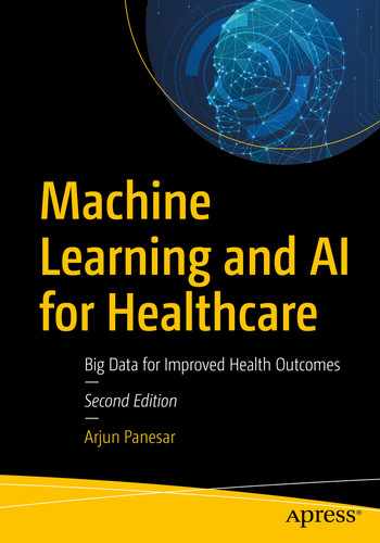
Ensembles
An ensemble is a form of machine learning algorithm and is a popular technique employed in the field of machine learning. Ensemble methods use a collection of machine learning models or learners. As a result, a group of weak learning models is combined to create a more accurate learning model.
There are two types of ensemble techniques—bagging and boosting.
Bagging
Bagging vs. boosting
In bagging, n′ < n samples are taken from dataset D with replacement. A random selection of features for constructing the best split is chosen each time.
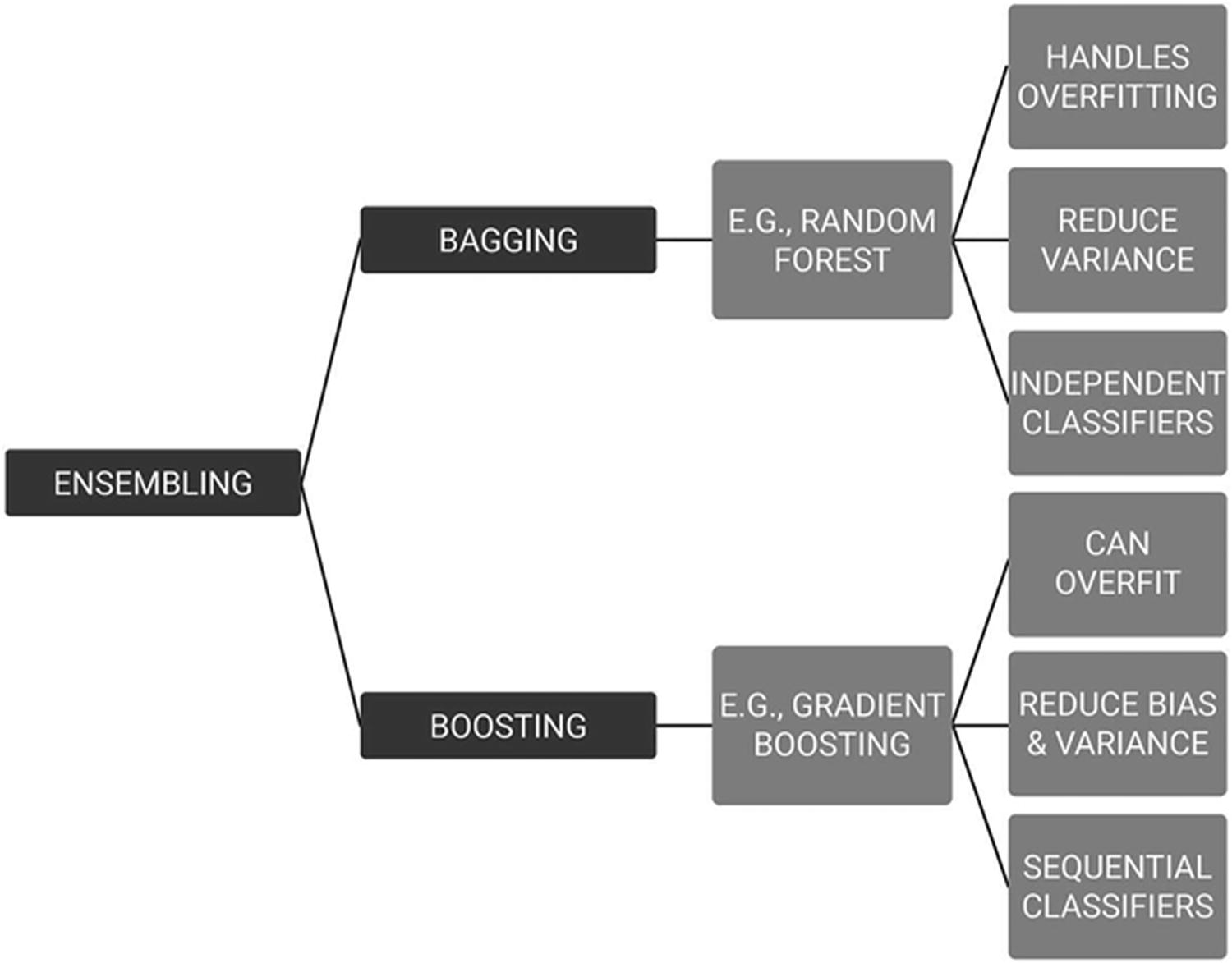
Random forest decision trees
Random Forest Decision Trees
Python, scikit-learn; method, RandomForestClassifier
Random forest decision trees are an example of bagging. Random forests are created through training multiple decision trees at the same time and refer to a collection of decision tree learners (hence the “forest”). The purpose of random forests is to prevent overfitting. The more decision trees in the random forest, the more accurate results are.
Each random forest takes a sample of the dataset and a random subset of features for decision.
Random forest decision trees can be used for classification and regression problems. With regression problems, an average of the outcomes is taken; whereas with classification problems, it is the majority category. A random forest decision tree is an ensemble of different models. This is an ensemble method due to the procedure reducing variance in the algorithm through combining predictions from multiple models.
The random forest model seems to work particularly well when data is limited to classification or decision problems by bootstrapping existing data. A benefit of random forest classifiers is that they can also handle missing values.
Boosting
Boosting is an ensemble method that produces a collection of predictive models iteratively. The concept involves each new model learning from the errors of previous models.
Boosted methods are typically implemented when there is a plethora of data for prediction.
Through iteratively creating new models to compensate for error, the process “boosts” or converts weak learners into strong learners—reducing their bias and variance. Each iteration of the technique learns relationships in the data and is then subsequently analyzed for errors, with incorrect classifications given a weighting. The aim is to minimize the error from the previous model. The underlying machine learning method used for boosting algorithms can be anything.
- 1.
Data is represented.
- 2.
Decision stump is made on the most significant cut of features.
- 3.
Weightings are given to misclassified observations.
- 4.
The process is repeated and all stumps combined to achieve the final classifier.
Gradient Boosting
Python, scikit-learn; method, GradientBoostingClassifier, GradientBoostingRegressor
Gradient boosting is known by many names including multiple additive regression trees, stochastic gradient boosting, and gradient boosting machines. Gradient boosting is a technique derived from decision trees when Jerome Friedman applied the gradient boosting concept to decision trees in 2001 [77]. AdaBoost (Freund and Shapire, 2001) is a gradient boosting variant. In gradient boosting, the model is trained sequentially. Each iterative model seeks to minimize the loss function [78].
Similar to random forest decision trees, gradient boosting is made from weak predictors. Each new tree is subsequently trained with the data previously incorrectly classified by the previous tree. This iterative procedure expedites the model by focusing on more challenging data as easier predictions are made early on in learning.
XGBoost, or extreme gradient boosting, is a variation of gradient boosting. XGBoost adds regularization and takes advantage of computing power with distributed, multithreaded processing for greater speed and efficiency.
Adaptive Boosting
Python, scikit-learn, numpy; method, AdaBoostClassifier, AdaBoostRegressor
Adaptive boost is a popular method that iteratively learns from mistakes. Decision tree stumps are weak learners, splitting data by one rule only. The decision tree stump is improved by focusing on samples that were incorrectly classified. These are identified through weightings that are associated with the data. The model can learn from its mistakes and provides a final solution with lower bias than a single decision tree.
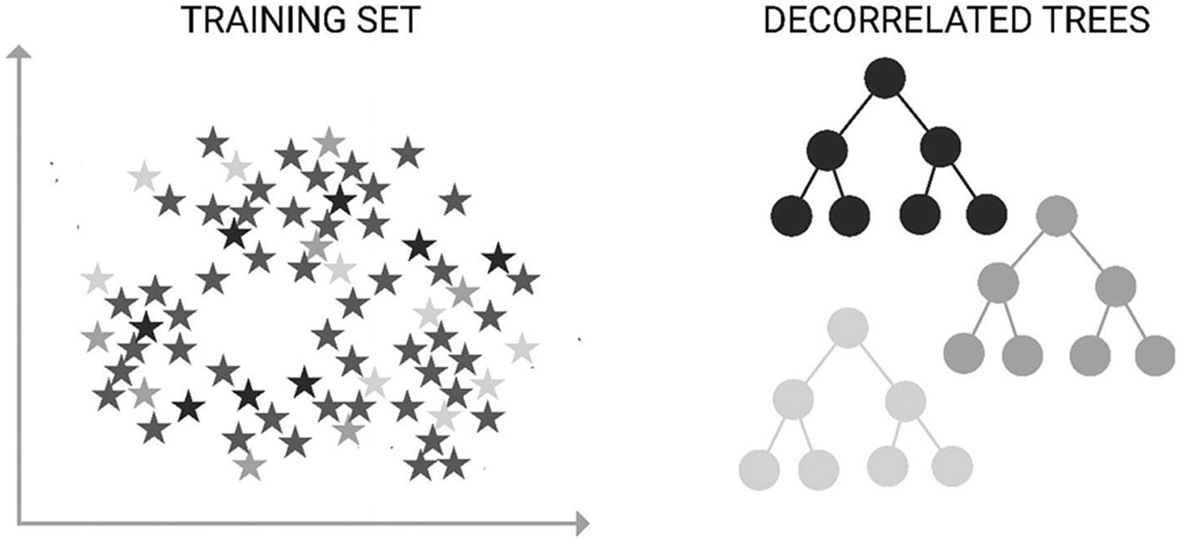
Linear Regression
Python, scikit-learn; method, linear_model.LinearRegression
Linear regression

 is the predicted value of the response variable, and their subtraction is the residual variation or difference between observed and predicted values of y.
Criterion variable: Outcome variable we are predicting
Predictor: What variable predictions are based on
Intercept: Where the line of best fit intercepts the y-axis

where y is the output variable, x is the predictor, B0 and B1 are coefficients that are estimated to move the line of best fit,  refers to the mean of x, B0 is the bias or intercept (where it intercepts the y-axis), and B1 is the slope or rate at which y increases/decreases per unit of x.
Once the model has learned the parameters, they are used to predict values of y given new, unseen input X.
Popular techniques used to estimate the coefficients are ordinary least squares and gradient descent. Given a line of best fit placed through a sample dataset with a linear relationship, ordinary least squares attempts to minimize the sum of the squared distances from each data point to the regression line. The intention is to minimize the sum of squared residuals. Coefficient values are iteratively optimized to reduce the error of the model.
Ordinary least squares starts with random values for B0 and B1. The sum of squared errors is calculated for each (input, output) pair. A learning rate is chosen, which acts as a scale factor; and the coefficients are optimized toward minimizing the error until no further gains can be made.
A learning rate is a hyperparameter that has its value determined by experimentation. Different values are tried, and the value that gives the best results is used.
Criticisms of linear regression focus on its simplicity, resulting in it being unable to capture complex relationships within the data. Noise in the data can also be learned by the model, resulting in overfitting.
Relationships between variables are not always linear, and therefore, a linear regression model can perform poorly on data with nonlinear relationships. However, variables can sometimes be transformed to fit a linear regression model. Linear regression also assumes variables are homoscedastic, which means all variables in the vector have the same variance.
The aforementioned is a perfect demonstration as to why when training a model, one should use a variety of machine learning algorithms.
Logistic Regression
Python, scikit-learn; method, linear_model.LogisiticRegression
Linear regression applies to continuous variables, whereas logistic regression predictions apply to discrete values or classification problems after the application of a transformation function.
Developed by statistician David Cox in 1958, logistic regression (or logit regression) is often used for binary classification problems. For example, logistic regression can be used to predict whether a patient will experience an adverse event given a particular medication, whether a patient is likely to be readmitted to a hospital or not, or whether a patient has a particular disease diagnosis.
Unlike linear regression, the output of the model comes in the form of a probability between 0 and 1. The predicted output is generated by log-transforming the x input and using the logistic function h(x) = 1/(1 + e^ – x). A specified threshold is used to transform this probability into a binary classification.

Logistic function
Sigmoid function: 1/(1 + e^–value), where e is Euler’s number and value is the value requiring transformation.
Logistic regression uses an equation P(x) = e ^ (b0 + b1*x)/(1 + e^(b0 + b1*x)), which can be transformed into ln(p(x)/1–p(x)) = b0 + b1*x). As with linear regression, b0 and b1 are values learned from the training data.
As an example, take a model that determines whether a growth on the skin surface is benign or not. The input variable, x, could be the size, depth, or texture of the growth; and the default variable y = 1 indicates a benign growth. As depicted, the logistic function transforms the x-value of the various instances into a probability value between 0 and 1. If the probability crosses the threshold of 0.5, the tumor is classified as benign.
Logistic regression seeks to learn values of b0 and b1 through training that minimize the error between predicted and actual outcomes. Maximum likelihood estimation is an iterative procedure used for this purpose.
Maximum likelihood estimation starts with a random value as the best weight for each predictor variable and then adjusts these coefficients iteratively until there is no improvement in the ability to predict the outcome value. The final coefficients have a value that minimizes the error in the probabilities predicted.
As with linear regression, logistic regression assumes a linear relationship between input variables and output. Feature reduction may be required to transform data into linear models. Logistic regression models are also prone to overfitting, which may be overcome through the removal of highly correlated inputs.
Finally, it is possible that coefficients fail to converge, which can happen if data is sparse or highly correlated.
SVM
Python, scikit-learn; method, svm.SVC, svm.LinearSVC
Support vector machine (SVM) is a nonprobabilistic binary linear classifier used with both classification and regression problems. SVM is often used along with NLP methods to analyze text for topic modeling and sentiment analysis. It is also used in image recognition problems and handwriting digit recognition.
The algorithm finds a hyperplane, or line of best fit, between two classes determined by the support vectors. Support vectors are the data points nearest the hyperplane that would alter the position of the hyperplane if removed. The greater the margin value, or distance from the data points to the hyperplane, the more confidence there is that the data is appropriately classified. The line of best fit is learned from an optimization procedure that seeks to maximize the margin.
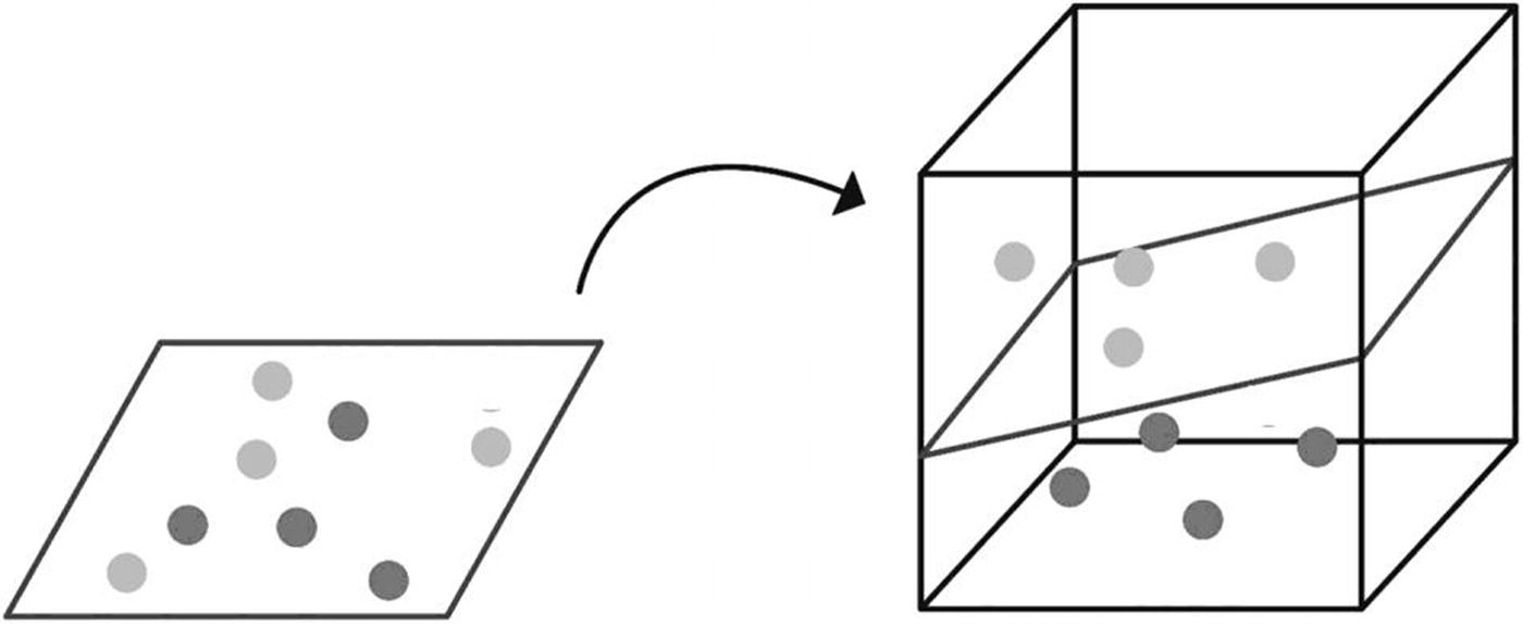
SVM uses something known as kernelling to map data to higher-dimensional feature spaces. Data is mapped using the kernel trick in iteratively more dimensions until a hyperplane can be formed to classify it.
SVM visualization
SVMs take numerical inputs and work well on small datasets. However, as dimensionality increases, the ability to understand and explain the model reduces. As dataset size increases, so too can training time. SVMs are also less capable on noisy data.
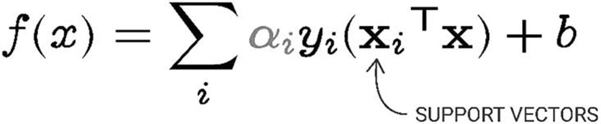
SVM expressed as a sum over the support vectors
Naive Bayes
Python, scikit-learn; method, GaussianNB, MultinomialNB, BernoulliNB
Naïve Bayes uses Bayes’s theorem to calculate the probability an event will occur given another event has already occurred. The algorithm is acknowledged as naïve because it assumes all variables are independent of each other, which is atypical of real-world examples. The Bayesian classifier is often used when input dimensionality is high.
For example, given a specified threshold, this method can be used to probabilistically classify whether a vector is in one class or another:
P(B|A) = Posterior probability (Figure 4-8): Probability of hypothesis B being true, given the data A, where P(B|A)= P(a1|b) * P(a2|b) * … * P(an|b) * P(A)
P(A|B) = Likelihood: The probability of data A given that the hypothesis B was true
P(A) = Class prior probability
P(B) = Predictor prior probability
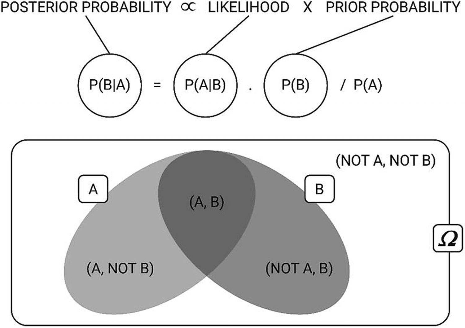
Posterior probability
The prior distribution P(B) and likelihood probability P(B|A) can be estimated from the training data. To calculate which class an example belongs to, the probability of being in each class is calculated. The class assigned to an example is the class that produces the highest probability for the example.
P(high risk|unhealthy)
= (P(high risk|unhealthy) * P(high risk))/P(unhealthy) = (2/2 * 2/4)/(3/4) = 0.66
Outcome likelihood
Record | Unhealthy | Outcome |
|---|---|---|
Person 1 | Yes | High risk |
Person 2 | Yes | Low risk |
Person 3 | Yes | High risk |
Person 4 | No | Low risk |
Naïve Bayesian models are easy to build and particularly useful for extensive datasets. Along with its simplicity (and hence its naïvety), naïve Bayes is known to outperform even highly sophisticated classification methods.
kNN: k-Nearest Neighbor
Python, scikit-learn; method, neighbors.KNeighborsClassifier
Not to be confused with k-means clustering, the kNN method classifies an unknown object O with the label of the majority of the k-nearest neighbors. Used in classification and regression problems, kNNs are a nonparametric technique. They do not learn a model. Instead, kNNs store the training dataset as their representation and perform classification of a new sample based on learning by analogy.
As there is no learning of the model, kNNs are considered lazy learners.

- 1.
Calculate the distance between any two points.
- 2.
Find the nearest neighbors based on these pairwise distances.
- 3.
Majority vote on a class label based on the nearest neighbors list.
The prediction is made at the time of the request. In regression problems, the mean or median of the k-most similar instances is used. In classification problems, the class with the highest frequency from the k-most similar instances is selected.
As with most algorithms, the determinant method can vary. The distance between binary vectors (Hamming distance) and the sum of absolute difference between real vectors (Manhattan distance) are also used.
A disadvantage of kNNs is the large computing requirement for classifying an object, as the distance for all neighbors in the training dataset must be calculated. It is not particularly well suited to high-dimensional data. Each predictor variable can be considered a dimension of N-dimensional input space. For instance, x1 would be one-dimensional and x1, x2 two-dimensional and so on. The increase in dimensionality exponentially increases the volume of the input space.
kNNs are not well suited to data with missing values, as distances between vectors cannot be calculated on missing data.
Neural Networks
The biological mechanism in which the brain works inspires artificial neural networks, a different paradigm for computing, based on the parallel architecture of animal brains.
Neural networks are well equipped for data mining tasks due to their ability to model multidimensional data and efficiency at finding hidden patterns among data. Neural networks can be applied to prediction and classification problems. The process of estimating the result and comparing it with the real output is known as forward propagation.
Neural networks are a subset of machine learning algorithms, which include perceptrons, fully connected neural networks, convolutional neural networks, recurrent neural networks (RNNs), long short-term memory neural networks, autoencoders, deep belief networks, generative adversarial networks, and many more. Most of them are trained with an algorithm called backpropagation.
Classifying disease—computers can learn what images of diseased organs, such as the kidneys, eyes, and liver, look like to predict the likelihood of disease
Recognizing speech
Translating and digitalizing text
Facial recognition
Neural networks can learn how to accomplish a task like a human brain—supervised, unsupervised, and through reinforcement learning.
Perceptron
Linear—such as the weighted sum
Threshold functions that only fire if the weighted sum is over a threshold
Step functions that output the inverse, typically –1, if S is less than the threshold
Sigma function (1/(1 + e – s), which allows for backpropagation
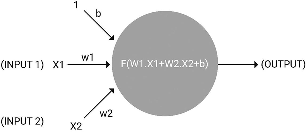
Configuration of an artificial neuron

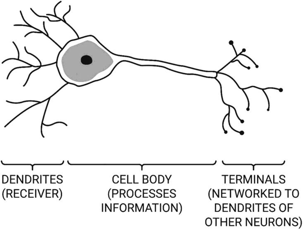
Configuration of a biological neuron
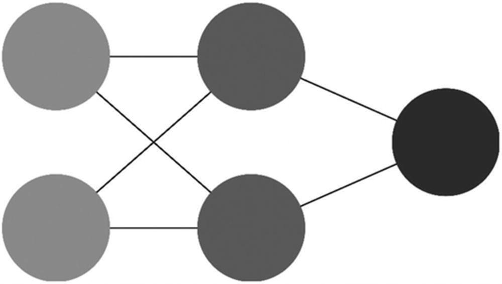
Artificial Neural Networks
Python, scikit-learn; method, linear_model.Perceptron

Organization of an artificial neural network
Backpropagation is the method of determining the error, or loss, at the output and propagating it back to the network. Weights at each node are updated to minimize the respective error output from each neuron. Backpropagation seeks to minimize the error for neurons and thereby the entire model through updating respective neuron weights.
The primary learning that must be accomplished in neural network models is training neurons when to fire. An epoch refers to one training iteration of forward- and backpropagation. During the learning phase, nodes in a neural network adjust their weights based on the error of the last test result. The learning rate controls how fast the network learns.
The number of perceptrons or neurons in a model are equal to the number of variables in the data. Some representations may also have a bias node.
Typically, artificial neural networks have neurons organized in layers. Each layer can perform different transformations on the input data it receives.
Deep Learning
Deep learning is a process that employs deep-layered neural network architectures. Training a deep, artificial neural network model requires more time and CPU power compared to other types of models. Noteworthy is that the performance of ANN models may not necessarily be superior to typical supervised learning techniques.
Deep learning is not a new technique; however, it is becoming more frequent with hardware advances, primarily power and cost, which have made such computing feasible.
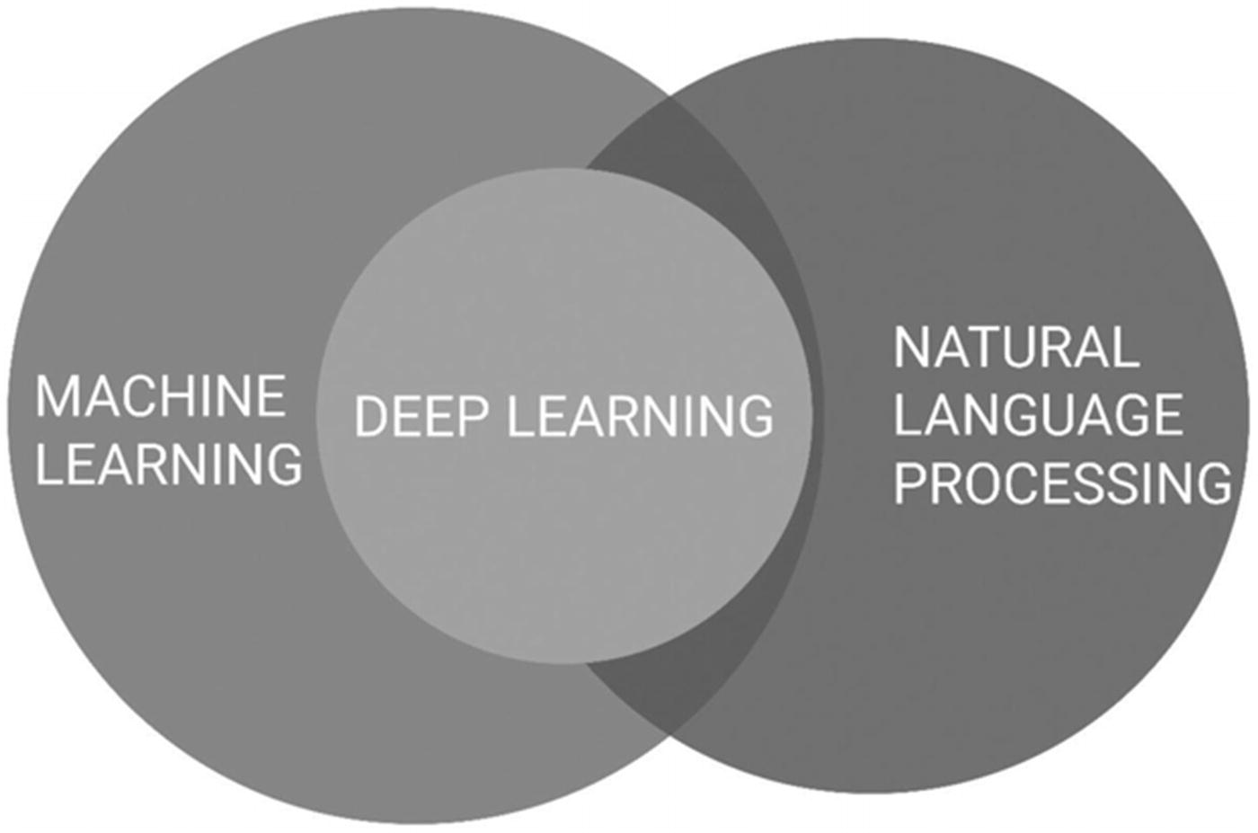
Deep learning: Where does it sit?
There are many types of artificial neural networks, including the following.
Feedforward Neural Network
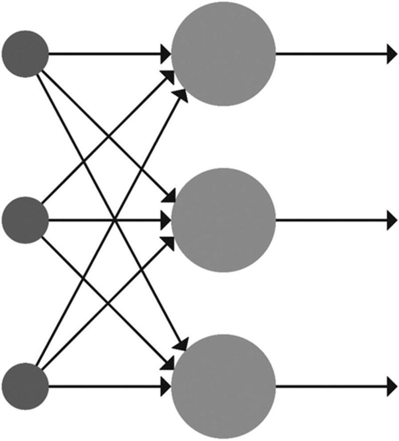
Feedforward neural networks
Recurrent Neural Network (RNN): Long Short-Term Memory
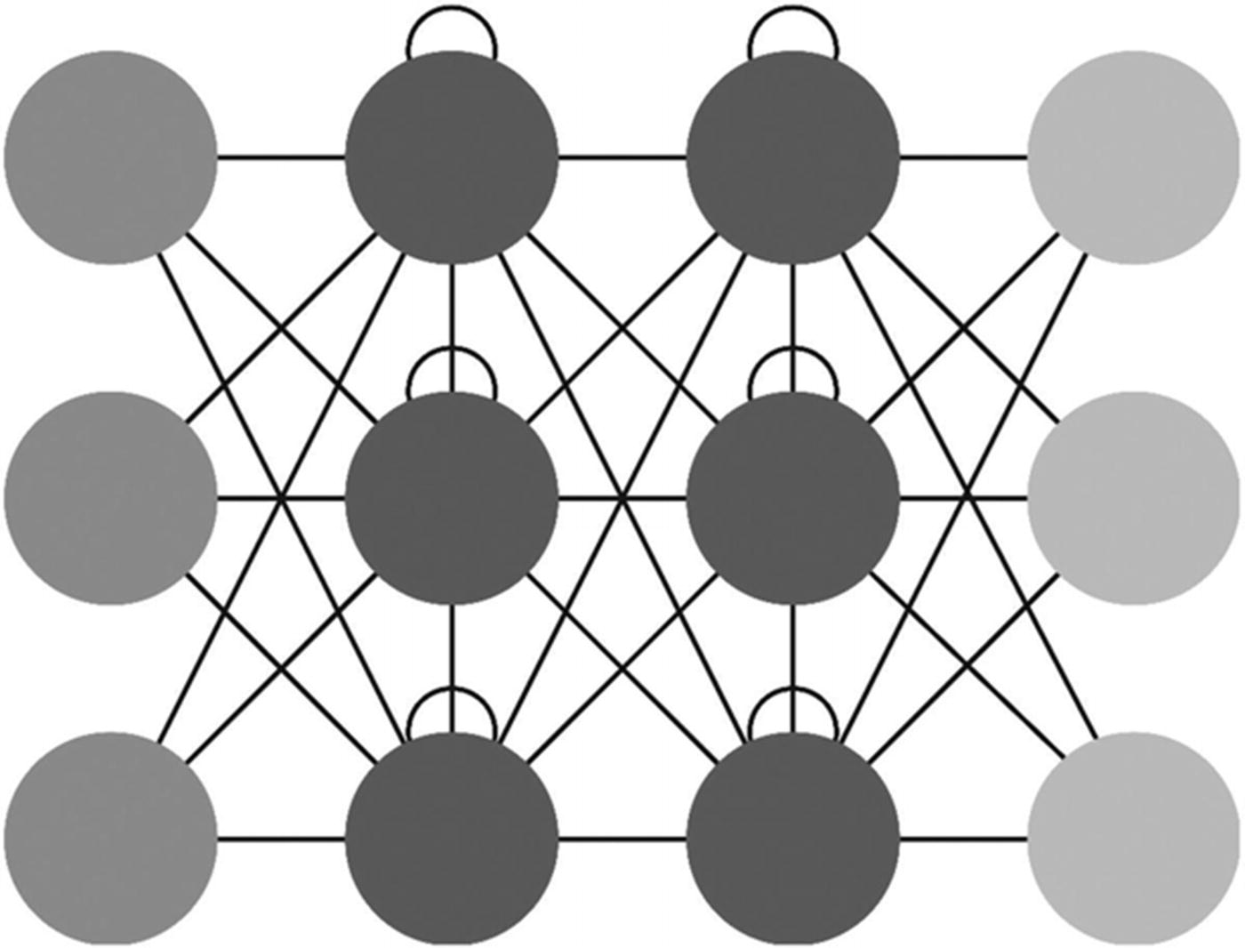
Recurrent neural networks
Convolutional Neural Network
Convolutional neural networks are deep, feedforward neural networks. Layers are known as convolutional layers and are often used in speech recognition, spatial data, NLP, and computer vision problems. Separate convolutional layers typically apply to different aspects of a particular problem.
For instance, in understanding whether there is a face present within a photograph, separate convolutional layers within a DNN may be used to identify different aspects of the face—the eyes, nose, ears, mouth, and so forth.
Modular Neural Network
Similar to the human brain, the concept of modular neural networks is that of neural networks working together.
Radial Basis Neural Network
Radial basis neural network
The key strength of ANNs and deep learning lies in the ability to generate complex linear and nonlinear models from the training dataset.
DNNs (deep and multilayered ANNs) can learn complex relationships between data from training data alone, which typically improves generalization. DNNs can still succumb to the problem of overfitting data, so appropriate pruning may be required. As the name suggests, deep networks can also take a long time to train and require a large number of training examples.
A common concern with neural networks, particularly in healthcare, is that they act as a black box and do not present a clear interface for a user to understand findings. Practically, an ANN model is difficult to interpret, and weights and biases aren’t readily interpretable to what is important in the model.
It is typically considered that for supervised learning problems, the upper bound on neurons to prevent overfitting is
Nh=Ns(〈 ∗(Ni + No)),
Ni = number of input neurons
No = number of output neurons
Ns = number of samples in the training dataset
〈 = an arbitrary scaling factor
Unsupervised Learning
Unsupervised learning refers to the process of learning a model from unlabeled data. This means that input data (x) is supplied without output (y). Algorithms are left to determine notes within data, which means there is no right or wrong answer.
Semi-supervised learning occurs when some output labels (y) are supplied. For example, learning would be semi-supervised in a model learning to predict glaucoma from patient eye scans with partially labeled data. If only a subset of eye scans had appropriately labeled outputs (e.g., glaucoma, not glaucoma), the model might not have enough appropriate data to learn a model. As more labeled data is provided for the model to train on, the system would likely become more accurate.
Unsupervised learning can be resource consuming concerning time, money, and expertise. Usually, vast improvements in model accuracy can be made through improving labeling of data.
Unsupervised learning is composed of two main problem concepts: clustering and association.
Clustering
Grouping patients of similar profiles together for monitoring
Detecting anomalies or outliers in claims or transactions
Defining treatment groups based on medication or condition
Detecting activity through motion sensors
k-Means
Python, scikit-learn; method, cluster.KMeans
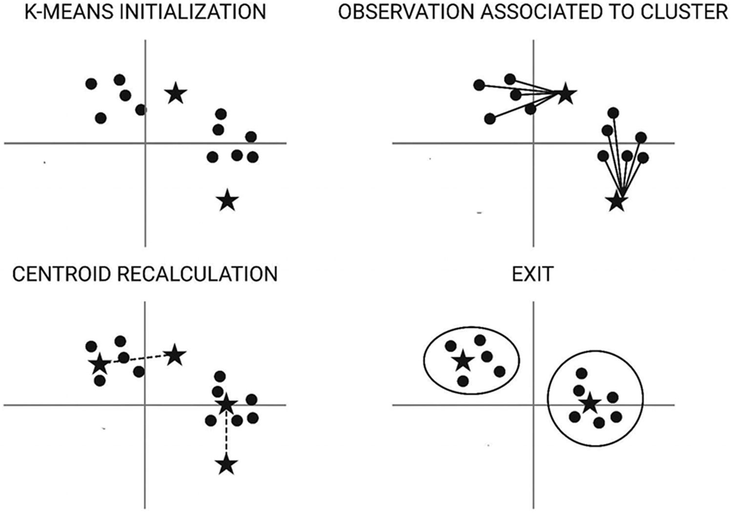
k-Means clustering

where ci is the collection of centroids in set C and distance (dist) is standard Euclidean distance.
Rather than defining groups before data exploration, clustering enables the model to determine groups that have formed organically.
- Step 1: Set a value of k. Here, let us take k = 2.
Assign each data point randomly to any of the k = 2 clusters.
Determine the centroid for each of the clusters.
Step 2: For each data point, associate it to the closest cluster centroid.
Step 3: Recalculate centroids for the new clusters.
Step 4: Continue this process until the centroid clusters remain unchanged.
Association
Association rule learning methods extract rules that best explain perceived relationships between variables in data. These rules can discover useful associations in large multidimensional datasets that can be used to drive and optimize.
Association rule learning is historically best applied to online shopping checkout basket datasets gathered on users’ purchasing habits. For instance, when someone buys a pizza, they may also tend to purchase wine, just like how someone who purchases lettuce may tend to buy tomatoes, cucumbers, and onion too. Through analyzing transactional datasets, the probability of associations can be predicted. We know that certain items (whether that be food, clothes, or even disease) frequently occur together, and association rule learning seeks to understand these relationships.
In healthcare, in particular, associative symptoms can be understood to predict better and diagnose disease and adverse events. Determining potential adverse effects based on medication and associative patient comorbidity pathways could lead to improved care and treatment pathways.
There are three important metrics to be familiar with.
Support
sup = Pr(X U Y) = count(X U Y)/Total transaction count
Confidence
conf = Pr(Y|X) = count(X U Y)/count(X)
Lift
Lift = Support (X U Y)/Support (X) * Support (Y)
Association rules determine the probability of Y given that X occurs. The benefits of these associations have applications across industry. There are many association rule mining algorithms that use different strategies toward understanding associations and use different structuring of data.
Apriori
Apriori is the most popular association rule mining algorithm. The Apriori algorithm is frequently used in pattern mining and in the identification of features and items that occur together. It is used extensively in basket analysis and is a powerful tool to find hidden feature patterns. It is usually applied to transactional databases to mine frequent relationships and generate association rules.
Apriori begins with a set of n items. The algorithm calculates all possible candidate itemsets, or frequent itemsets, which meet the specified threshold support and confidence values. The Apriori property states for an itemset to be frequent, all of its subsets must also be frequent. The Apriori algorithm uses a bottom-up approach; frequent subsets are identified and increased one item at a time.
Apply minimum support to find all frequent sets of k items within dataset T where a frequent itemset has support ≥ min(sup).
Expand selection to find frequent sets of k + 1 items using frequent k-itemset.
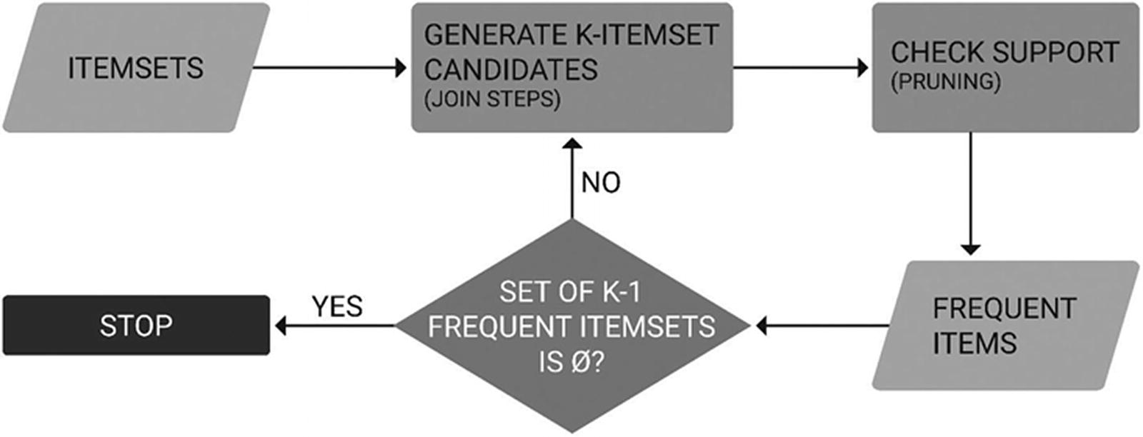
Apriori
The maximum size of an itemset is k, the number of items.
Dimensionality Reduction Algorithms
Although the message is broadly the more data, the better, datasets can often contain many variables and as a result make capturing the signal of the data a more laborious task. Whether it’s sparse values, missing values, identifying relevant features, resource efficiency, or more straightforward interpretation, dimensionality reduction algorithms are very useful to data scientists.
Mobile phones collect hundreds of data points including calls, texts, steps, calories burned, floors climbed, Internet usage, and so forth. What data is best for understanding phone usage?
Brands on social media are collecting data on engagement and interactions such as comments, likes, followers, sentiment, and mood. What data is best for understanding attitudes toward health?
Medical health records contain a wealth of information, but only some information is relevant in predicting disease risk or illness progression. What data is relevant to understanding future risk of disease or adverse event?
Dimensionality reduction refers to converting a dataset of many dimensions into fewer dimensions while concisely representing similar data.

Dimension reduction
Dimensions of value can be identified or combined or new dimensions created to represent the inherent relationships.
Fewer dimensions result in quicker computations when compared to the original dataset.
By default, dimension reduction algorithms reduce the space required for storage.
Reducing data into fewer than three dimensions enables visualization and easier understanding.
Redundant data is removed, which improves the performance of the machine learning model.
Noise is removed, which improves model performance.
Dimension Reduction Techniques
Dimension reduction can be achieved in a variety of ways.
Missing/Null Values
Missing data and null values are not a huge problem in isolation, but a growing number of empty values may help determine whether to drop a variable, ignore missing values, or compute a predicted value.
Most data scientists support the dropping of variables if an attribute has upward of 50% empty or null values. This threshold does vary.
Low Variance
Data attributes that are very similar to one another do not carry much information. As a result, there is little variance within the data. Hence, a lower variance threshold can be set and dimensions removed based upon this.
As variance is dependent on range, data normalization should take place first.
High Correlation
Attributes with similar data trends are likely to carry similar information. Multicollinearity is the carrying of similar information that can reduce the performance of the model. Correlation between continuous data is determined by the Pearson product-moment coefficient, which is a measure of the linear correlation between two variables X and Y.
For discrete data, the Pearson’s chi-square value determines how likely it is that any observed difference between sets arose by chance.
Random Forest Decision Trees
Random forest decision tree ensembles are useful for identifying key features. Random forest decision trees use a subset of features that can identify best split attributes.
If an attribute is often selected as the best split node, it is likely to be a feature to keep. Decision trees are particularly useful for visualizing reductions also.
Backward Feature Elimination
In Backward Feature Elimination , the model trains on n attributes. Starting with n attributes, at each iteration, the model is trained on n-1 attributes n number of times. The attribute that demonstrates the smallest increase in error rate is removed, and the algorithm performs another iteration on n-1 attributes.
At each iteration k, a model with n-k attributes is trained. This is computationally expensive.
Forward Feature Construction
Forward Feature Construction is the opposite of Backward Feature Elimination. The model starts with one attribute and evaluates which of the attributes has the highest increase in performance. Much like it’s opposite Backward Feature Elimination, this method is computationally expensive unless operating in a lower range of dimensions.
Principal Component Analysis (PCA)
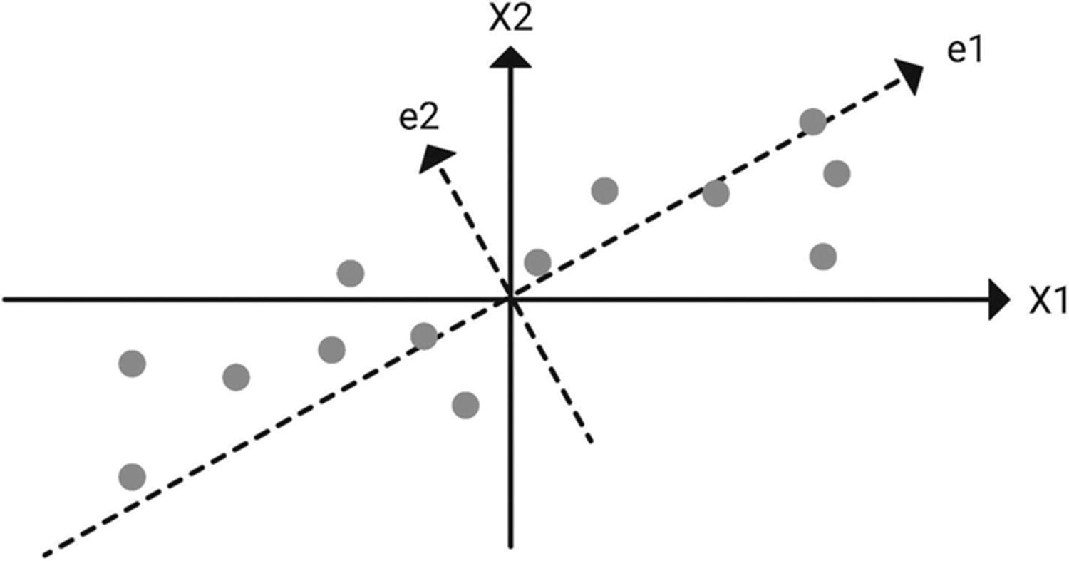
PCA
Each component is orthogonal and a linear combination of original variables. Orthogonality indicates that the correlation between the components is zero.
The first principal component is the linear combination of the original dimension that has the maximum variance; and the nth principal component is the linear combination with the highest variance, subject to being orthogonal to the n – 1 principal components .
Natural Language Processing (NLP)
Natural language processing is the field of AI that focuses on language. Natural language processing or NLP is defined as the ability of systems to analyze, understand, and generate human language, including speech and text.
The retrieval of structured and unstructured data within a dataset, for example, searching clinical notes by keyword or phrase
Social media monitoring
Question answering: interpretation of natural language from humans to interact appropriately, for instance, as with virtual assistants or speech recognition software
Analysis of a document to determine key findings
Ability to parse and interpret a text to understand sentiment and mood
Recognizing distinctions among diagnoses and relationships
Image to text recognition, for instance, reading a sign or menu
Machine translation—NLP is used in machine translation programs in which one human language is automatically translated into another human language
Topic modeling—what is this document talking about?
Understanding sentiment from social media or discussion posts
Interpreting natural language is fraught with challenges, as human language is naturally ambiguous—language, pronunciation, expression, and perception .
Although there are rules with human language, they are often misunderstood and misused. NLP takes into consideration the structure of language to derive meaning. Words make phrases; phrases make sentences; sentences make documents; and all of the aforementioned convey ideas.
NLP has a toolkit of text processing procedures including a range of data mining methods that can be used for model development. Due to the nature of unstructured data, NLP tasks can be expensive regarding computational resource and time. Neural networks and deep learning can also be used for NLP tasks.
With most data generated existing in the form of unstructured data, NLP is a powerful tool to interpret and understand natural language.
Tokenization: The process of converting a corpus of text into smaller units, or tokens. There are many algorithms available for breaking a text into tokens.
Tokens: Words or entities present in the text.
Text object: A sentence or a phrase or a word or an article.
Stemming: A basic rule-based process of stripping suffixes (“ing,” “ly,” “es,” “s,” etc.) from words.
Stem: The text created after stemming.
Lemmatization: Determining the root of a word from dictionaries and morphological analysis.
Morpheme: Unit of meaning in a language.
Syntax: Arranging symbols (words) to make a sentence. It involves determining the structural role of words in the sentence and phrases.
Semantics: Meaning of words and how to join words into meaningful phrases and sentences.
Pragmatics: Using and understanding sentences in different situations and how interpretations are affected.
In this section, I aim to introduce key concepts and methods of NLP and to demonstrate the techniques that can be applied to datasets to generate defined value .
Getting Started with NLP
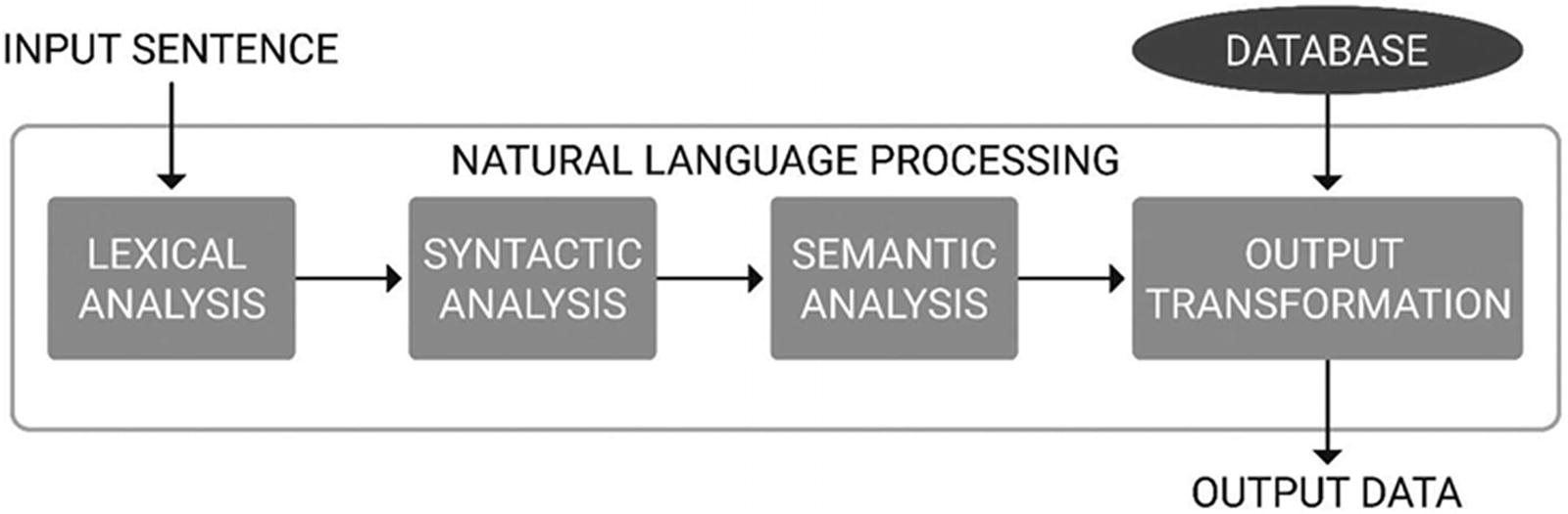
How NLP works
Preprocessing: Lexical Analysis
As with any dataset, a corpus of text that is not relevant to the context of data can be understood as noise. The first stage in NLP is to clean and standardize the input text, ensuring it is noise-free and ready for analysis.
Over and above spelling correction and grammar correction, the following techniques are used to reduce noise.
Noise Removal
Noise removal involves preparing a dictionary of noisy tokens (i.e., words) and parsing the text, removing the tokens found in the noise dictionary. For instance, words like the, a, of, this, that, and so forth would be removed.
Lexicon Normalization
Follow, following, followed, and follower are all variations of the word follow. Contextually, the words are similar. Lexicon normalization reduces dimensionality through stemming, which strips suffixes and prefixes, and lemmatization, which is a defined procedure that uses word structure and grammar relationships.
Porter Stemmer
Python, NLTK; method, PorterStemmer
The Porter stemmer algorithm is a popular and useful method to improve the effectiveness of information retrieval [81]. The algorithm works on the principle that many words in English share a common root. Stemming works on suffixes and removes common morphological and inflexional endings from words. Therefore, stemming allows one to reduce similar words into a common root form.
For example, take the text “I felt troubled by the fact that my best friend was in trouble. Not only that, but the issues I had dealt with yesterday were still troubling me.”
The words troubled, trouble, and troubling all share the common root trouble. Therefore, according to the Porter stemmer algorithm, instead of counting all three words once, the stem trouble is counted thrice instead. The benefit of stemming is that common words can be clustered under a common stem to provide a more accurate statistical representation of the number of occurrences of a certain word. However, a drawback of stemming is that the semantic meaning of the word may be lost.
Stemming and lemmatization are used to reduce inflectional forms and sometimes derivationally related forms of a word to a common base form.
Object Standardization
A corpus of text may contain words that cannot be found in lexicon dictionaries. For example, on Twitter, someone may mention DM’ing someone, or another may like an RT of someone else’s tweet. Acronyms, hashtags, slang, and colloquialisms can be removed through prepared dictionaries or using regular expressions.
Syntactic Analysis
To be analyzed, the text needs to be converted into features. The syntactic analysis of text involves analyzing sentences to understand relationships between words and assigning a syntactic structure to it. There are several algorithms for syntactic analysis; however, the Context-Free Grammar is most popular due to it being the simplest style of grammar and therefore widely used.
Take the sentence “David saw a patient with uncontrolled type 2 diabetes.”
Within the sentence, we need to identify the subject, objects, noise, and attributes to understand the sequence of words and its dependencies.
Dependency Parsing
Toolkit, NLTK; method, StanfordDependencyParser

Dependency parsing
Dependency grammar analyzes asymmetrical binary relationships between tokens. The Stanford parser from NLTK is commonly used for this purpose.
Using the example in Figure 4-21, the parse tree determines the root of the word as “saw” and is then linked by subtrees. The subtrees are split by subject and object, with each subtree also showing dependencies .
Part of Speech Tagging
Toolkit, NLTK; method, word_tokenize
Part of speech (POS) tagging involves associating each word or token in a sentence with a part of speech tag. These tags are the basic English labels that you learned in primary school and determine nouns, verbs, adjectives, adverbs, numbers, and so on.
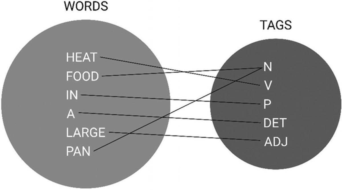
Part of speech tagging
Part of speech tagging is the basis of the assists in several areas .
Reducing Ambiguity
Some sentences have multiple meanings given the structure; for example, take the following two sentences:
“I managed to read my book on the train.” “Can you please book my train tickets?”
Part of speech tagging identifies “book” as a noun in the first sentence and as a verb in the second sentence.
Identifying Features
By identifying the types of speech alongside different contexts of a word, POS can distinguish between uses and creates stronger features for use.
Normalization
POS tags are the foundation of normalization and lemmatization, to understand sentence structure and dependency.
Stopword Removal
POS is useful in removing commonly used words, or stopwords, from a text.
Semantic Analysis
Semantic analysis is the most complex phase of NLP. It draws the exact meaning or the dictionary meaning from the text. Using knowledge about the structure of words and sentences among the context, the meaning of words, phrases, sentences, and texts is stipulated, and subsequently, also their purpose and consequences.
Techniques Used Within NLP
Once data preprocessing, lexical, syntactical, and semantic analysis of corpus has taken place, we are required to transform text into mathematical representations for evaluation, comparison, and retrieval. For instance, searching a collection of patient profiles for users with “hypertension” should only bring out those with hypertension. This is achieved through transforming documents into the vector space model with scoring and term weighting essential for query ranking and search retrieval.
Documents can be in the form of patient records, web pages, digitalized books, and so forth. The following algorithms are typical in the comparison and evaluation process.
N-Grams
Python: NLTK; Method: ngrams

David reversed
Reversed his
His metabolic
Metabolic syndrome
N-Grams preserve the sequences of N items from the text input. N-Grams can have a different N value: unigrams for when N = 1, bigrams when N = 2, and trigrams when N = 3.
N-Grams are used extensively for spelling correction, word decomposition, and summating texts.
TF–IDF Vectors

Each term’s weight (Wtd) is calculated by multiplying the frequency of the term (ftd) by the log of the total number of documents (D) divided by the number of documents the term occurs at least once in (NDt). The ordering of the terms may not necessarily be maintained.
Weights for the terms gathered can then be used to determine documents with high frequencies of the specific term within them. A collection of TF–IDF vectors could be used to represent a user’s interest.
Latent Semantic Analysis
Where there is a corpus of a large number of documents, for each document d, the dimension of the vector representing each document can typically exceed several thousand. Latent semantic analysis relies on the fact that intuitively, terms in documents may often be related. For example, if document d contains the term sea, it will often contain the word beach.
Equivalently, if the vector representing d has a non-zero component in the entry for sea, it will also have a non-zero component in the beach entry. If this kind of structure can be detected, relationships between words can be automatically learned from the data.
The word document is represented by a matrix A, which is decomposed using singular value decomposition to give the strength of the most significant correlations and their directions.
The decomposition of A allows one to discover the semantics of the document through correlations between terms and their significance within the document. The latent semantic analysis method can be applied to determine the context of a variety of materials to present a web user with results that are contextually relevant.
Cosine Similarity
Python, SciPy; method, cosine
The cosine similarity is a metric that measures the similarity between two vectors. Therefore, this could either be used to define the similarity between two documents or a document and a query.

The similarity between two vectors is calculated as the inner product of the vectors divided by the product of the lengths of the vectors in question. Intuitively, the greater the angle between two documents, the less similar they are. This holds for vectors in any N-dimensional space.

The similarity between a query q and document d is calculated as the product of the TF–IDF weights for the term in both the document and query summed over all the terms in both the query and document; this is divided by the product of the length of the document and length of the query. Practically, however, calculating Sim(q,d) would prove computationally expensive as the number of documents used grows.
Naïve Bayesian Classifier
The Bayesian classifier is based on the Bayesian theorem and is particularly suited when the dimensionality of the inputs is high. Despite its simplicity, naïve Bayes can often outperform more sophisticated classification methods.

Other techniques such as kNN and ANN can also be used to classify and retrieve information.
Genetic Algorithms
Genetic algorithms (GA) are a fascinating topic within machine learning. GA take inspiration from evolution to minimize the error rate, attempting to mimic the function of chromosomes much like neural networks attempt to mimic the human brain.
Evolution is considered the optimal learning algorithm. In machine learning, the application of this is in models whereby several candidate answers (referred to as chromosomes or genotypes) are produced and the cost function applied to all.
In GA, a fitness function is defined that determines if the chromosomes fit enough to mate. Chromosomes furthest away from the optimal outcome are removed. Chromosomes are also subject to mutation. GA are a type of search and optimization learner and apply to discrete and continuous problems.
Chromosomes that are close to the optimal solution may be combined. The combination or mating of chromosomes is known as a crossover. The survival of the fittest approach identifies chromosomes that aim to express characteristics that adhere to natural selection—where the offspring is more optimal than the parent.
Mutation helps to overcome overfitting. It is a random process to get over local optima and find the global optimum. Mutation helps to ensure that child chromosomes are different from the parents’ and continue evolution.
The degree in which chromosomes mutate and mate is a parameter that can be controlled or left to the model to learn.
Detection of blood vessels in ophthalmology imaging
Detecting the structure of RNA
Financial modeling
Routing vehicles
A group of chromosomes is referred to as a population. Although it stays at a defined, constant size, it usually evolves to better average predictions over the course of generations or time.
fitness(c) = g(c)/(Average of g over the entire population)
John Holland invented the GA approach (see Figure 4-23) in the early 1970s [81]. The automation of chromosome selection is known as genetic programming.
Best Practices and Considerations
Mastering the art of machine learning takes time and experience. However, there are several areas worthy of consideration, particularly for beginners to machine learning, to ensure the best use of time and optimal model efficiency.
Good Data Management

Basic structure of a genetic algorithm
Establish a Performance Baseline
It is crucial to have a baseline to measure the performance of your algorithm against other iterations and model types. As there is no one perfect algorithm for every problem, attempt many algorithms to identify the relative performance of your models.
Spend Time Cleaning Your Data
The time required to train a machine learning model varies significantly between algorithms. The accuracy of data and time spent on training the model positively influence model accuracy. Take time to clean your data to ensure predictions are as robust as possible.
It is often the case that not all of the input variables impact the dependent variable or outcome. Ensure the variables used by the model do not include those that are irrelevant.
Training Time
If the dimensionality of data is large and computing power limited, training time will be extensive. When time is short, it is useful to consider machine learning algorithms that do not require substantial training. For example, neural networks may not be appropriate for time-limited tasks.
Choosing an Appropriate Model
Some machine learning algorithms make particular assumptions about the structure of data or the desired outputs. For this reason, it is helpful to consider the model choice and whether it is an appropriate approach. Utilizing the right model has a plethora of benefits, including more accurate predictions, faster training times, and more useful results.
Some machine learning models are resistant to outliers or nonparametric tests. For example, decision tree–based approaches typically classify a node into two based on a threshold. Data outliers are therefore less impactful in tree-based approaches.
Evaluating a range of models is a useful approach to machine learning. Occam’s razor is typically applied to choosing the model of choice. Occam’s razor seeks to identify the most straightforward model that achieves the desired output given all else being equal.
Choosing Appropriate Variables
Although more data is ordinarily invited in machine learning problems, it is typically preferable to work with fewer predictor variables for many reasons.
Redundancy
Increasing the number of variables within a training dataset increases the chances of models learning hidden relationships between them. It is vital to identify unnecessary variables and only use nonredundant predictor variables within models. A model that is learning redundant connections will impact model accuracy.
Overfitting
Even if there are no relationships among predictor variables within a model, it is still beneficial to use fewer variables. Complex models, or those that use a high number of predictor variables, typically suffer from overfitting.
Models perform well on training datasets but are less accurate on validation and real-world settings, as they learn the error within the data (i.e., the noise) rather than the signal, or relationships, between variables.
Productivity
Even if all of the variables within a sophisticated machine learning model are relevant, there is a practical impact in using a large number of predictor variables that can affect productivity.
Practical considerations include the amount of data available, the subsequent effect on storage, computing resources, associated costs, time allocated for the project, and the time required for learning and validation. Predictor variables can be identified through feature selection, or transformed through feature extraction. SVMs are useful in cases of increased data dimensionality.
The Pareto principle (or the 80/20 rule or law of a vital few) is a useful measure to use in machine learning projects. Using the Pareto principle, focusing on the 20% most significant predictor variables should facilitate the building of relatively successful models within a reasonable time. Microsoft learned that 80% of the errors and crashes in Windows and Office were caused by 20% of the entire set of bugs detected [82].
The “Pareto principle” is the observation that approximately 80% of the effects come from 20% of the causes. Many natural phenomena have been shown empirically to exhibit such a distribution.
Understandability
Models with fewer predictor variables are easier to visualize, understand, and explain. A key aspect of a successful machine learning project is that all stakeholders can comprehend the model. This often requires data scientists trading off.
By reducing the number of predictor variables, there is a chance there may be a reduction in the success of a machine learning model. However, this concurrently makes the model easier to interpret and understand.
The usefulness of this approach is only realized toward the end of a project when it comes to sharing not only the performance of a model but also how it works. This is particularly relevant in healthcare, as there are concerns about using black box models.
Accuracy
Any machine learning model aims to generalize well. Depending on the use case, an approximation may be more beneficial than a precise, accurate output. Through approximating values, models tend to avoid overfitting and reduce the amount of time spent on processing.
Impact of False Negatives
When evaluating the impact of a model before deployment into a live environment, consider the impact of false negatives. For example, take a predictive model that classifies the risk of breast cancer. A false positive would mean that a patient is informed they have breast cancer when they do not, which should be identified later in the treatment pathway. However, a false negative would mean a patient with breast cancer would not be notified—which is potentially far worse and costly.
Linearity
Many machine learning algorithms assume that relationships are linear—in other words, that classes can be separated by a straight line of best fit or its higher-dimensional representation. There are instances where relationships are not linear. Relying on a linear classification algorithm where there is a nonlinear class boundary will result in low accuracy.
Linear regression, for example, assumes both input and output variables do not contain noise. It is vital to expose the signal within data to ensure models learn the signal or the correct relationships within the data. It is advantageous to identify and remove outliers for the output variable in particular to reduce the chances of learning the noise.
Data with a nonlinear trend may require transforming to make the relationship linear, for instance, log-transforming data where there is an exponential relationship.
Linear algorithms are typically the first methods attempted in machine learning scenarios. As a result of linearity, algorithms are simple and quick to train.
Parameters
Each machine learning model is subject to parameters and hyperparameters. The time and resource required to train a model increases as the number of parameters does. An algorithm’s parameter is a variable that is utilized by the model where the value can be estimated from the dataset.
An algorithm’s hyperparameter is a variable that is external to the model and used to estimate parameters. A hyperparameter’s value cannot be estimated from data. Instead, it is set by the data scientist, randomly or otherwise, or through the use of heuristics.
Ensembles
In specific machine learning problems, it may prove more useful to group classifiers together using the techniques of voting, weighting, and combination to identify the most accurate classifier possible. Ensemble learners are very useful in this aspect.
Use Case: Toward Smart Care in Diabetes
Type 2 diabetes is one of the most significant health and economic burdens facing the global population, with one in six people dying from diabetes or its related complications every 6 seconds [83, 84].
There are many factors involved in the progression of the disease, which, if tackled, can help to prevent its progression through targeted treatment profiling, leading to lower patient morbidity and mortality rate. Data in the form of health biomarkers—typically blood glucose, HbA1c, fasting blood glucose, insulin sensitivity, and ketones—are used to understand and monitor disease burden and response to treatments.
As a result of the tremendous burden of type 2 diabetes, there has been a substantial investment in developing intelligent models within this area, with much of the focus on diagnosing, predicting, and managing the condition through machine learning and data mining.
Many machine learning techniques have been applied to type 2 diabetes datasets. Traditional techniques, ensemble techniques, and unsupervised learning—in particular, association rule mining—have been used to identify prediction models with optimal accuracy.
Predicting Blood Glucose
Georga, E. I. et al. used random forest decision trees on many features collected from 15 people with type 1 diabetes to predict short-term subcutaneous glucose concentrations [85]. Glucose concentration was predicted through the use of SVMs.
The study concluded that the inclusion of two biomarker features—8-hydroxy-2-deoxyguanosine, an oxidative stress marker, and interleukin-6—improved classification accuracy.
Predicting Risk
Farideh Bagherzadeh-Khiabani et al. used the clinical dataset from 803 female prediabetics consisting of 55 features collected over a decade to develop multiple models for predicting type 2 diabetes risk [86]. The study developed a logistic model, demonstrating wrapper models, or models that consider a subset of features and improve the performance of clinical prediction models. This was developed into an R program to visualize output.
Summers, Panesar, et al. developed a model consisting of 34 features collected for people with prediabetes and obesity to predict risk of developing type 2 diabetes based on the health and engagement outcomes of over 200,000 people who used the Low Carb Program digital health intervention. This was developed in Python and deployed on the cloud to assess patient risk and suitability for the award-winning digital therapy [16, 58].
Razavian et al. conducted another extensive study, determining that type 2 diabetes prediction models could be accurately derived from population-scale datasets [87]. Over 42,000 variables were collected from over 4 million patients between 2005 and 2009. Machine learning was used to determine relevant features, which tailed out at around 900. Novel risk factors for type 2 diabetes were identified, such as chronic liver disease, high alanine aminotransferase, esophageal reflux, and history of acute bronchitis.
Duygu Çalişir et al. developed an automatic diagnosis system for type 2 diabetes with a classification accuracy of almost 90% through the use of linear discriminant analysis and SVM classifiers [86]. Latent Dirichlet Allocation (LDA) was used to distinguish features between healthy patients and patients with type 2 diabetes, which was then in turn used as the input for the SVM classifier. A tertiary stage evaluated sensitivity, classification, and confusion before determining the output.
Predicting Risk of Other Diseases
Machine learning has likewise been applied to diagnosing the risk of other diseases related to diabetes.
Lagani et al. identified the least set of clinical variables with the best predictive accuracy for complications such as cardiovascular disease (heart disease or stroke), hypoglycemia, ketoacidosis, proteinuria, neuropathy, and retinopathy [88].
Huang et al. used decision tree–based prediction models on identifying diabetic nephropathy in patients [89]. Leung et al. compared several methods: partial least square regression, regression trees, random forest decision trees, naïve Bayes, neural networks, and SVMs on genetic and clinical features [90]. Patient age, years of diagnosis, blood pressure, genetic polymorphisms of uteroglobin, and lipid metabolism arose as the most efficient predictors of type 2 diabetes.
Summers et al. developed a predictive model utilizing a dataset consisting of over 120 features to identify comorbid depression and diabetes-related distress. Summers et al. explored several techniques including random forest decision trees, SVMs, naïve Bayes, and neural networks. Patient age and employment status were defined as the variables most likely to affect predictive accuracy [16, 86].
Unsupervised learning has mainly concentrated on association rule mining, identifying associations between risk factors in people with diabetes. Simon et al. proposed an extension to association rule mining labeled survival association rule mining, which included survival outcomes, and made adjustments for confounding variables and dosage effects [86].
Reversing Disease
The understanding of type 2 diabetes has been radically disrupted by the generation of real-world evidence over the last 15 years. Previously, type 2 diabetes was understood as a chronic, progressive disease.
The Low Carb Program digital health intervention has been instrumental in demonstrating that sustainable weight loss is achievable through scalable digitally delivered therapies, supporting prediabetes and type 2 diabetes remission. The platform’s peer-reviewed evidence shows 54% reduce or eliminate diabetes medications, with retention of 71% at 1 year.
A key driver in the Low Carb Program’s success has been the implementation of a predictive model to identify education modules, resources, recipes, and discussion threads that are most likely to engage patients. This results in the app itself showing a different experience to each patient based on key features including ethnicity, age, gender, location, language, weekly food budget, dietary preferences, health status, and comorbidities.
This uses the patient’s data to provide personalized, tailored care to best empower decisions and provide around-the-clock support. The benefits of this approach are self-evident, with one in four patients achieving type 2 diabetes remission at 1 year. Outcomes from Low Carb Program have been used to influence public nutrition policy and guidelines. The app was ranked the #1 app for diabetes in the NHS [91, 92].
Machine learning is so often focused on predicting and diagnosing disease. The application of machine learning to reverse disease provides hope that we can support improved behaviors and redefine outdated paradigms.