
Chapter 6. Protecting the Consumer Web
Most of our discussion so far has focused on preventing hackers from getting into a computer or network, detecting them after they’ve achieved a breach, and mitigating effects of the breach. However, it is not necessary for an attacker to breach a network in order to gain economically. In this chapter we consider attackers who use a consumer-facing website or app’s functionality to achieve their goals.
When referring to the “consumer web,” we mean any service accessible over the public internet that provides a product to individual consumers; the service can be free or fee-based. We distinguish the consumer web from enterprise services provided to an organization, and from internal networks within a company.
The consumer web has many different attack surfaces; these include account access, payment interfaces, and content generation. Social networks provide another dimension of vulnerability, as attackers can take advantage of the social graph to achieve their goals.
However, the consumer web also has some built-in properties that work to the defender’s advantage. The foremost of these is scale: any site that is subject to attack is also subject to a much larger amount of legitimate traffic. This means that when building your defense, you have a large database of legitimate patterns you can use to train your algorithms. Anomaly detection, as discussed in Chapter 3, can be appropriate here, especially if you don’t have a lot of labeled data. On the other hand, if you are considering building defenses into your product, it’s probably because your website or app has already undergone an attack—in which case you probably have enough labeled data to build a supervised classifier.
In the subsequent sections, we consider various attack vectors and how machine learning can help distinguish legitimate activity from malicious activity in each case. Because open source consumer fraud data is scarce, we will focus primarily on principles behind feature generation and algorithm selection for each problem; toward the end of the chapter, we will use a concrete example to illustrate approaches to clustering.
Even though the title of this chapter is “Protecting the Consumer Web,” everything we discuss applies equally to websites accessed via a browser and apps that get their data from an internet-facing API. In the following sections we will consider some of the differences in attack surface and features available to the defender.
Monetizing the Consumer Web
Many consumer-facing websites make it possible for hackers to monetize directly simply by gaining access to an account. Financial institutions are the most obvious example, but online marketplaces, ride-sharing services, ad networks, and even hotel or airline rewards programs also facilitate direct transfers of currency to essentially arbitrary recipients. Hackers need only compromise a few high-value accounts to make the investment worthwhile. Protecting accounts on such a service is thus paramount for the site’s continued existence.
Fraud is another key concern for many consumer-facing websites. Most online services accept credit cards for payment, and thus bad actors can use stolen credit cards to pay for whatever the sites offer. For sites that offer consumer goods directly this is particularly dangerous, as the stolen goods can then be resold on the black market for a fraction of their retail price. Even sites that offer digital goods are susceptible to fraud; digital goods can be resold, or premium accounts on a service can be used to accelerate other types of abuse on that service.
Fraud encompasses much more than payments. Click fraud consists of bots or other automated tools clicking links for the sole purpose of increasing click counts. The most prominent use case is in advertising, either to bolster one’s own revenue or to deplete competitors’ budgets; however, click fraud can appear anywhere where counts influence ranking or revenue, such as number of views of a video or number of “likes” of a user’s post. We also consider review fraud, whereby users leave biased reviews of a product to artificially inflate or deflate that product’s rating. For example, a restaurant owner might leave (or pay others to leave) fake five-star reviews of their restaurant on a dining site to attract more customers.
Even if a hacker can’t monetize directly, there are a large number of sites that provide indirect means to monetization. Spam is the most obvious—any site or app that provides a messaging interface can be used to send out scams, malware, or phishing messages. We discussed text classification of spam messages in Chapter 1 and thus won’t go into further detail here; however, we will discuss behavior-based detection of spammers. More generally, any site that allows users to generate content can be used to generate spammy content; if this content is in broadcast form rather than user-to-user messaging, other fraud or search engine optimization (SEO) techniques can expose the spam to a broad audience. The attacker can even take advantage of social signals: if popular content is ranked more highly, fake likes or shares allow spammers to promote their message.
This list of activities covers most of the abuse on the consumer web but is far from exhaustive. For further information, we recommend the Automated Threat Handbook from the Open Web Application Security Project (OWAS) as a good resource that describes a large variety of different types of abuse.
Types of Abuse and the Data That Can Stop Them
Let’s now examine in more depth some of the different ways in which attackers can try to take advantage of consumer websites. In particular, we will look at account takeover, account creation, financial fraud, and bot activity. For each of these attack vectors we will discuss the data that needs to be collected and the signals that can be used to block the attack.
Authentication and Account Takeover
Any website or app that only serves content does not need to make any distinction between users. However, when your site needs to differentiate the experience for different users—for example, by allowing users to create content or make payments—you need to be able to determine which user is making each request, which requires some form of user authentication.
Authentication on the internet today overwhelmingly takes the form of passwords. Passwords have many useful properties, the foremost of which is that due to their prevalence, nearly everyone knows how to use them. In the ideal situation, passwords serve to identify a user by verifying a snippet of information that is known only to that user. In practice, however, passwords suffer from many flaws:
-
Users choose passwords that are easy to remember but also easy to guess. (The most common password seen in most data breaches is “password.”)
-
Because it is nearly impossible to remember a unique, secure password for each site, people reuse passwords across multiple sites; research has shown that nearly half of all internet users reuse credentials.1 This means that when a site is breached, up to half of its users are vulnerable to compromise on other unrelated sites.
-
Users are vulnerable to “phishing” campaigns, in which a malicious email or website takes on the appearance of a legitimate login form, and tricks users into revealing their credentials.
-
Users might write down passwords where they can be easily read or share them with friends, family, or colleagues.
What are websites to do in the face of these weaknesses? How can you ever be sure that the person logging in is the actual account owner?
One line of research has focused on developing alternative authentication mechanisms that can replace passwords entirely. Biometric identifiers such as fingerprint or iris scans have been shown to be uniquely identifying, and behavioral patterns such as typing dynamics have also shown success in small studies. However, biometrics lack revocability and are inherently unchangeable. Because current sensors are susceptible to being tricked, this brittleness makes for an unacceptable system from a security standpoint, even leaving aside the difficult task of getting users to switch away from the well-known password paradigm.
A more common pattern is to require a second factor for login. This second factor can be deployed all the time (e.g., on a high-value site such as a bank), on an opt-in basis (e.g., for email or social sites), or when the site itself detects that the login looks suspicious. Second factors typically rely on either additional information that the user knows or an additional account or physical item that the user possesses. Common second-factor authentication patterns include:
-
Confirming ownership of an email account (via code or link)
-
Entering a code sent via SMS to a mobile phone
-
Entering a code generated by a hardware token (such as those provided by RSA or Symantec)
-
Entering a code generated by a software app (such as Google Authenticator or Microsoft Authenticator)
-
Answering security questions (e.g., “What month is your best friend’s birthday?”)
-
Verifying social information (e.g., Facebook’s “photo CAPTCHA”)
Of course, all of these second factors themselves have drawbacks:
-
Email accounts are themselves protected by passwords, so using email as a second factor just pushes the problem to the email provider (especially if email can be used to reset the password on the account).
-
SMS codes are vulnerable to man-in-the-middle or phone-porting attacks.
-
Hardware and software tokens are secure but the user must have the token or app with them to log in, and the token must be physically protected.
-
Social details can often be guessed or found on the internet; or the questions might be unanswerable even by the person owning the account, depending on the information requested.
In the most extreme case, the website might simply lock an account believed to be compromised, which requires the owner to contact customer support and prove their ownership of the account via an offline mechanism such as verifying a photo ID.
Regardless of the recovery mechanism used, a website that wants to protect its users from account takeover must implement some mechanism to distinguish legitimate logins from illegitimate ones. This is where machine learning and statistical analysis come in.
Features used to classify login attempts
Given the aforementioned weaknesses of passwords, a password alone is not enough to verify an account holder’s identity. Thus, if we want to keep attackers out of accounts that they do not own, whenever we see a correct username–password pair we must run some additional logic that decides whether to require further verification before letting the request through. This logic must run in a blocking manner and use only data that can be collected from the login form. It must also attempt to detect all of the types of attacks discussed earlier. Thus, the main classes of signals we want to collect are as follows:
-
Signals indicating a brute-force attack on a single account:
-
Velocity of login attempts on the account—simple rate limiting can often be effective
-
Popularity rank of attempted passwords—attackers will try common passwords2
-
Distribution of password attempts on the account—real users will attempt the same password or similar passwords
-
-
Signals indicating a deviation from this user’s established patterns of login:
-
Geographic displacement from previous logins (larger distances being more suspicious)
-
Using a browser, app, or OS not previously used by the account
-
Appearing at an unusual time of day or unusual day of the week
-
Unusual frequency of logins or inter-login time
-
Unusual sequence of requests prior to login
-
-
Signals indicating large-scale automation of login:
-
High volume of requests per IP address, user agent, or any other key extracted from request data
-
Unusually high number of invalid credentials across the site
-
Requests from a hosting provider or other suspicious IP addresses
-
Browser-based telemetry indicating nonhuman activity—e.g., keystroke timing or device-class fingerprinting
-
Engineering all of these features is a nontrivial task; for example, to capture deviations from established patterns, you will need a data store that captures these patterns (e.g., all IP addresses an account has used). But let’s assume you have the ability to collect some or all of these features. Now what?
First of all, let’s consider brute-force protection. In most cases a simple rate limit on failed login attempts will suffice; you could block after a certain threshold is reached or require exponentially increasing delays between attempts. However, some services (e.g., email) might have apps logging in automatically at regular intervals, and some events (e.g., password change) can cause these automated logins to begin to fail, so you might want to discount attempts coming from a known device.
Depending on your system’s security requirements you might or might not be able to get some data on the passwords being entered. If you can get a short-term store of password hashes in order to count unique passwords attempted, you can rate limit on that feature, instead. You might also want to lock an account for which many passwords attempted appear in lists obtained from breaches.
Now we consider attacks in which the attacker has the password. The next step depends on the labeled data you have available.
Labeling account compromise is an imprecise science. You will probably have a set of account owners who have reached out complaining of their accounts being taken over; these can be labeled as positives. But assuming there is some (perhaps heuristic) defense mechanism already in place, how do you know which accounts you stopped from logging in were truly malicious, as opposed to those with legitimate owners who couldn’t (or didn’t bother to) get through the additional friction you placed on the account? And how do you find the false negatives—accounts taken over but not yet reported as such?
Let’s assume you don’t have any labeled data. How do you use the signals described here to detect suspicious logins?
The first technique you might try is to set thresholds on each of the aforementioned features. For example, you could require extra verification if a user logs in more than 10 times in one hour, or more than 500 miles from any location at which they were previously observed, or using an operating system they haven’t previously used. Each of these thresholds must be set using some heuristic; for example, if only 0.1% of users log in more than 10 times per hour, you might decide that this is an acceptable proportion of users to whom to apply more friction. But there is a lot of guesswork here, and retuning the thresholds as user behavior changes is a difficult task.
How about a more principled, statistical approach? Let’s take a step back and think about what we want to estimate: the probability that the person logging in is the account owner. How can we estimate this probability?
Let’s begin by estimating an easier quantity from the login data: the probability that the account owner will log in from the particular IP address in the request. Let u denote the user in question and x denote the IP address. Here is the most basic estimate of the probability:
Suppose that we have a user, u, who has the following pageview history:
| Date | IP address | Country |
|---|---|---|
1-Jul |
1.2.3.4 |
US |
2-Jul |
1.2.3.4 |
US |
3-Jul |
5.6.7.8 |
US |
4-Jul |
1.2.3.4 |
US |
5-Jul |
5.6.7.8 |
US |
6-Jul |
1.2.3.4 |
US |
7-Jul |
1.2.3.45 |
US |
8-Jul |
98.76.54.32 |
FR |
For the login on July 6, we can compute the following:
But what do we do with the login on July 7? If we do the same calculation, we end up with a probability estimate of zero. If the probability of user u logging in from IP x is zero, this login must be an attack. Thus, if we took this calculation at face value, we would need to regard every login from a new IP address as suspicious. Depending on the attacks to which your system is exposed and how secure you want your logins to be, you might be willing to make this assumption and require extra verification from every user who changes IP addresses. (This will be particularly annoying to users who come from dynamically assigned IPs.) However, most administrators will want to find some middle ground.
To avoid the issue of zero probabilities, we can smooth by adding “phantom” logins to the user’s history. Specifically, we add β login events, α of which are from the IP address in question:
The precise values of α and β can be chosen based on how suspicious we expect a new IP address to be, or, in statistical terms, what the prior probability is. One way to estimate the prior is to use the data: if 20% of all logins come from IP addresses not previously used by that user, values of α = .2 and β = 1 are reasonable.3 With these values, the logins from our imaginary user on July 6 and 7 get probability estimates of, respectively:
Note that if we just look at IP addresses, the logins on July 7 and 8 are about equally suspicious (P = 0.03 for both). However, it is clear from the table that the July 8 login should be treated with more suspicion because it’s from a country not previously visited by that user. This distinction becomes clear if we do the same calculation for country as we did for IP address—if we let α = .9 and β = 1 for the smoothing factors, the logins on July 7 and 8 have, respectively, probability estimates of:
This is a significant difference. We can use similar techniques for all of the features labeled earlier as “signals indicating a deviation from established patterns of login”: in each case, we can compute the proportion of logins from this user that match the specified attribute, adding appropriate smoothing to avoid zero estimates.
How about the “large-scale automation” features? To calculate velocity features, we need to keep rolling counts of requests over time that we can look up on each incoming request. For example, we should keep track of the following (among others):
-
Number of successful/failed login attempts sitewide in the past hour/day
-
Number of successful/failed login attempts per IP address in the past hour/day
-
Number of successful/failed login attempts per user agent in the past hour/day
To determine whether there is an unusually high number of invalid credentials across the site you can do the following: calculate the login success rate for each hour over a sufficiently large historical period, and use this data to compute the mean and standard deviation of the success rate. Now when a login comes in, you can compute the success rate over the past hour and determine whether this value is acceptably close to the historical mean; if you’re using heuristics, failure rates two or three standard deviations above the mean should trigger alerts or additional friction. To get a probability, you can use a t-test to compute a p-value. You can compute similar statistics on failure rate per IP or failure rate per user agent.
Finally, we consider the “requests from a suspicious entity” features. To accurately capture these features you need reputation systems that assign to each entity (e.g., IP address) either a label or a score that indicates the prior level of suspicion. (For example, hosting providers would typically have low scores.) We defer the discussion of how to build reputation systems to later in this chapter.
Building your classifier
Now that you have all these features, how do you combine them? Without labels, this task is a difficult one. Each feature you have computed represents a probability, so the naive approach is to assume that all of the features are independent and simply multiply them together to get a total score (equivalently, you can take logs and add). A more sophisticated approach would be to use one of the anomaly detection techniques from Chapter 3, such as a one-class support vector machine, isolation forest, or local outlier factor.
With labels, of course, you can train a supervised classifier. Typically, your labels will be highly unbalanced (there will be very little labeled attack data), so you will want to use a technique such as undersampling the benign class or adjusting the cost function for the attack class.
Account Creation
Even though getting into a legitimate user’s account might be necessary to steal assets belonging to that user, attacks such as sending spam or fake content can be carried out from accounts created and owned by the attacker. If attackers can create a large number of accounts, your site could potentially be overwhelmed by illegitimate users. Thus, protecting the account creation process is essential to creating a secure system.
There are two general approaches to detecting and weeding out fake accounts: scoring the account creation request to prevent fake accounts from being created at all, and scoring existing accounts in order to delete, lock, or otherwise restrict the fake ones. Blocking during the creation process prevents attackers from doing any damage at all, and also keeps the size of your account database under control; however, scoring after the fact allows greater precision and recall, due to the fact that more information is available about the accounts.
The following (simplistic) example illustrates this trade-off. Suppose that you have concluded from your data that if more than 20 new accounts are created from the same IP address in the same hour, these accounts are certain to be fake. If you score at account creation time, you can count creation attempts per IP address in the past hour and block (or perhaps show a CAPTCHA or other challenge) whenever this counter is greater than 20. (See the following subsection for details on rolling counters.) However, for any particular attack, there will still be 20 fake accounts that got through and are free to send spam. On the other hand, if you score newly created accounts once per hour and take down any group of more than 20 from the same IP address, you will block all the spammers but still give them each one hour to wreak havoc.
Clearly a robust approach combines instances of both techniques. In this section, we consider a scoring model that runs at account creation time. The features that go into such a model fall into two categories: velocity features and reputation scores.
Velocity features
When an attacker is flooding your system with account creation requests, you don’t want to build a complicated machine learning model—you just want to block the offending IP address. But then the attacker will find a new IP address, and now it becomes a game of whack-a-mole. To avoid this game and create a robust, automated defense, we use velocity features.
The basic building block of a velocity feature is a rolling counter. A rolling counter divides time into k buckets (e.g., each hour of the day) and for each key in a keyspace (e.g., the set of all IP addresses) maintains the count of events for that key in each bucket. At set intervals (e.g., on every hour), the oldest bucket is cleared and a fresh bucket is created. At any point we can query the counter to get the number of events for a given key in the past t buckets (if t ≤ k).
However, since each bucket will hold roughly the same number of keys, having many fine-grained buckets could lead to an explosion in your storage requirements (e.g., if you have 1-minute counters, your hourly count will be more accurate than if you had 10-minute counters).
After you have rolling counters,4 you can begin counting account creation attempts by any number of different keys, at one or more granularities of time. Key types that you might want to count on include the following:
-
IP address or IP subnet
-
Geolocation features (city, country, etc.)
-
Browser type or version
-
Operating system and version
-
Success/failure of account creation
-
Features of the account username (e.g., substrings of email address or phone number)
-
Landing page in the account creation flow (e.g., mobile versus desktop)
-
API endpoint used
-
Any other property of the registration request
You can also cross features: for example, successful desktop registrations per IP address. The only limits are your imagination and the allowable write throughput of your counter system.
Now that you’ve implemented counters, you can compute velocity features. Simple velocities are straightforward: just retrieve the counts from a certain number of buckets, sum them up, and divide by the number of buckets (perhaps with a conversion to your preferred unit). If you have a global rate limit on any feature, it’s easy to check, on any request, whether the current rate is above your limit.
Of course, global rates can go only so far. Most likely you have a small fraction of users on Linux and a much larger fraction on macOS. If you had a global limit on accounts created per OS per hour, this limit would need to be large enough to accommodate the macOS registrations, and a spike in the number of accounts created from Linux would go unnoticed.
To get around this problem, you can use historical data to detect unusual numbers of requests on any key. The rolling counter itself provides some historical data—for example, if you have counts of requests per hour for the past 24 hours, you can compute the quantity as follows:
Equation 6-1. Computing recent spikes
This formula gives you a “spike magnitude” of the past k hours compared with the previous 24 – k hours. (The +1 in the denominator is smoothing that prevents division by zero.) To find a reasonable threshold you should log or simulate the rolling counters on historical data and determine at what level you can safely block requests.
Using recent data to detect spikes will work only if there is enough of it. A more robust measurement will use historical data, computed from offline logs or long-term persistent counters, to establish a baseline of activity per key, per day, and then use a formula analogous to Equation 6-1 to determine when a quantity spikes. You must still take care to handle unseen or rare keys; smoothing the counts (as discussed in “Features used to classify login attempts”) can help here.
Detecting spikes is an example of a more general principle: velocities can be very effective when combined into ratios. Spike detection on a single key uses the ratio of recent requests to older requests. But any of the following ratios should have a “typical” value:
-
Ratio of success to failure on login or registration (failure spikes are suspicious)
-
Ratio of API requests to page requests (the API being hit without a corresponding page request suggests automation, at least when the user agent claims to be a browser)
-
Ratio of mobile requests to desktop requests
-
Ratio of errors (i.e., 4xx response codes) to successful requests (200 response code)
You can use rolling counters to compute these ratios in real time and therefore incorporate them as features in your classifier.
Reputation scores
Velocity features are good at catching high-volume attacks, but what if the attacker slows down and/or diversifies their keys to the point where the requests are coming in below the threshold for any given key? How can we make a decision on a single request?
The foundation here is the concept of reputation. Reputation quantifies the knowledge we have about a given key (e.g., IP address) either from our own data or from third parties, and gives us a starting point (or more formally, a prior) for assessing whether a request from this key is legitimate.
Let’s look at the example of IP address. The simplest reputation signal for a registration defense model is the fraction of accounts on that IP that have been previously labeled as bad. A more sophisticated system might capture other measures of “badness”: how many account takeover attempts have been seen from the IP, or how much spam has been sent from it. If these labels are not readily available, you can use proxies for reputation:
-
How long ago was the IP first seen? (Older is better.)
-
How many legitimate accounts are on the IP?
-
How much revenue comes in from the IP?
-
How consistent is traffic on the IP? (Spikes are suspicious.)
-
What’s the ratio of reads to writes on the IP? (More writes = more spam.)
-
How popular is the IP (as a fraction of all requests)?
In addition to data you collect, there is a great deal of external data that can go into your reputation system, especially with regard to IP addresses and user agents. You can subscribe to a database that will inform you as to whether any given IP address belongs to a hosting provider, is a VPN or anonymous proxy, is a Tor exit node, and so on. Furthermore, there are a number of vendors who monitor large swaths of internet traffic and compile and sell IP blacklist feeds; these vendors typically will provide a free data sample so that you can evaluate whether their labels overlap with the abuse you see on your site.
With regard to user agents, there are published lists of known bot user agents and web scripting packages. For example, requests from curl, wget, or python-requests should be treated with extra suspicion. Similarly, if a request advertises itself as Googlebot, it is either the real Googlebot or someone pretending to be Googlebot in the hopes that your thirst for search engine optimization will result in you letting them through—but the real Googlebot is not likely to be creating any accounts!
Now let’s consider how to combine all of these features into a reputation score, again using IP address as an example. One question we could answer with such a score is, “What is the probability that this IP address will be used for abuse in the future?” To cast this question as a supervised learning problem we need labels. Your choice of labels will depend on exactly what you want to defend against, but let’s say for simplicity that an IP address is bad if a fake account is created on it in a period of n days. Our supervised learning problem is now as follows: given the past m days of data for an IP, predict whether there will be a fake account created on it in the next n days.
To train our supervised classifier, we compute features (starting with those described previously) for each IP for a period of m days and labels for the n days immediately following. Certain features are properties of the IP, such as “is hosting provider.” Others are time based, such as “number of legitimate accounts on the IP.” That is to say, we could compute the number of accounts over the entire n days, or for each of the n days, or something in between. If there is enough data, we could compute n features, one for each day, in order to capture trends; this aspect will require some experimentation.
If you are planning on retraining regularly (e.g., daily), validation on a held-out test set (i.e., a random subset of your data excluded from training) is probably sufficient. If retraining is sporadic (e.g., less often than every n days), you will want to be sure that your model is sufficiently predictive, so you should validate your model on the next n days of your training samples, as demonstrated in Figure 6-1.
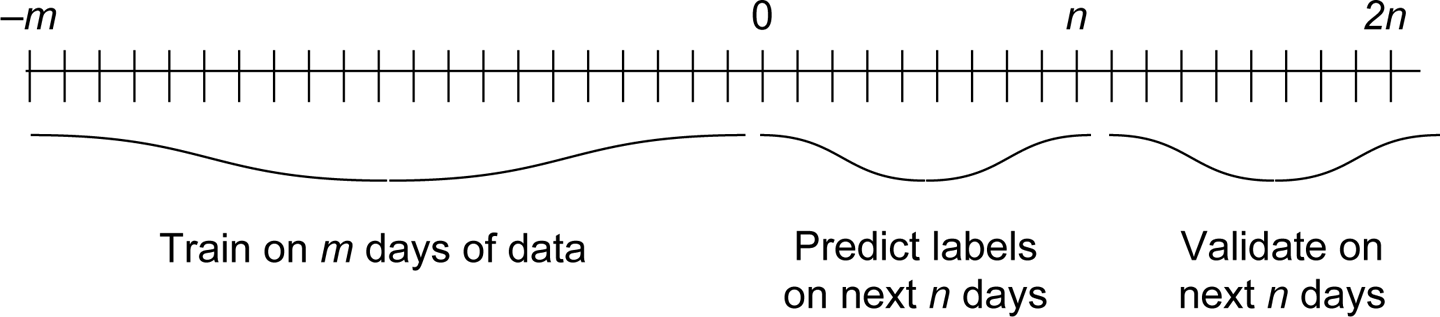
Figure 6-1. Out-of-time training and validation
A final word on reputation: we have for the most part used IP address in this section as our example. However, everything we wrote applies to any of the keys listed in the section “Velocity features” earlier in the chapter. The only limits to you creating reputation systems for countries, browsers, domains, or anything else are the amount of data you have and your creativity.
Financial Fraud
If attackers can obtain your product at no cost, they can resell it for less than your price and make money. This problem applies not only to physical goods that have a large secondhand market (e.g., electronics), but also to services that can be arbitraged in a competitive market (e.g., ride hailing). If your audience is large enough, there will be some people who try to steal your product regardless of what it is. To stop these people, you need to determine whether each purchase on your site is legitimate.
The vast majority of financial fraud is conducted using stolen credit cards. Credit card fraud is older than the internet, and an enormous amount of work has been done to understand and prevent it. A single credit card transaction passes through many different entities as it is processed:
-
The merchant (you)
-
A payment processor
-
The merchant’s bank
-
The card network (Visa/Mastercard/American Express/Discover), which routes inter-bank transactions
-
The card issuer’s bank
Each of these entities has fraud detection mechanisms in place, and can charge upstream entities for fraudulent transactions that make it to them. Thus, the cost of fraud to you is not just the loss of your product or service, but also fees assessed at different levels of the ecosystem. In extreme cases, the damage to your business’s credit and reputation may cause some banks or networks to levy heavy fines or even refuse to do business with you.
Of course, credit cards are not the only payment method you might accept on your site. Direct debit is a popular method in Europe, where credit cards are more difficult to get than in the United States. Many sites accept online payment services such as PayPal, Apple Pay, or Android Pay; in these cases, you will have account data rather than credit card and bank data. However, the principles of fraud detection are essentially the same across all payment types.
Although many companies offer fraud detection as a service, you might decide that you want to do your own fraud detection. Perhaps you can’t send sensitive data to a third party. Perhaps your product has an unusual payment pattern. Or perhaps you have calculated that it’s more cost effective to build fraud detection yourself. In any case, after you have made this decision, you will need to collect features that are indicative of fraud. Some of these include:
-
Spending profiles of customers:
-
How many standard deviations from the customer’s average purchase a given transaction is
-
Velocity of credit card purchases
-
Prevalence of the current product or product category in the customer’s history
-
Whether this is a first purchase (e.g., a free user suddenly begins making lots of purchases)
-
Whether this payment method/card type is typical for the customer
-
How recently this payment method was added to the account
-
-
Geographical/time-dependency correlation:
-
All the correlation signals for authentication (e.g., geographic displacement, IP/browser history)
-
Geographic velocity (e.g., if a physical credit card transaction was made in London at 8:45 PM and in New York at 9:00 PM on the same day, the user’s velocity is abnormally high)
-
-
Data mismatch:
-
Whether the credit card billing address matches the user’s profile information at the city/state/country level
-
Mismatch between billing and shipping addresses
-
Whether the credit card’s bank is in the same country as the user
-
-
Account profile:
-
Age of the user’s account
-
Reputation from account creation scoring (as just discussed)
-
-
Customer interaction statistics:
-
Number of times the customer goes through the payment flow
-
Number of credit cards tried
-
How many times a given card is tried
-
Number of orders per billing or shipping address
-
If you want to train a supervised fraud detection algorithm, or, even more basically, if you want to be able to know how well you’re doing at catching fraud, you will need labeled data. The “gold standard” for labeled data is chargebacks—purchases declared by the card owner to be fraudulent and rescinded by the bank. However, it usually takes at least one month for a chargeback to complete, and it can even take up to six months in many cases. As a result, chargebacks cannot be used for short-term metrics or to understand how an adversary is adapting to recent changes. Thus, if you want to measure and iterate quickly on your fraud models, you will need a supplementary metric. This could include any of the following:
-
Customer reports of fraud
-
Customer refunds
-
Purchases made by fake or compromised accounts
Finally, when building your system, it is important to think carefully about where in the payment flow you want to integrate. As with other abuse problems, if you wait longer you can collect more data to make a more informed decision but risk more damage. Here are some possible integration points:
- Preauthorization
-
You might want to run at least a minimal scoring before sending any data to the credit card company; if too many cards are declined, you might accrue fines. Furthermore, preauthorization checks prevent attackers from using your site as a test bed to determine which of their stolen cards work.
- Post-authorization, prepurchase
-
This is a typical place to run fraud scoring because it allows you to ignore cards that are declined by the bank and to avoid chargebacks, given that you won’t take funds for fraudulent purchases. If your site is set up with auth/capture functionality, you can let the customer proceed as if the purchase were going through, and collect more data to do further scoring before actually receiving the funds.
- Post-purchase
-
If you have a physical good that takes some time to prepare for shipping, or if you have a virtual service that cannot effect much damage in a short time, you can let the purchase go through and collect more behavioral signals before making a decision on the purchase and cancelling/refunding transactions deemed to be fraudulent. By scoring post-purchase, however, you are exposing yourself to chargebacks in the case that the real owner quickly discovers the fraud.
Bot Activity
In some cases, attackers can glean a great deal of value from a single victim. A bank account is an obvious example, but any account that can hold tradable assets is a target; these include ride- or house-sharing accounts, rewards accounts, or ad publishing accounts. For these high-value accounts it makes sense for attackers to work manually to avoid detection. On the other hand, in many cases the expected value of a single victim is very small, and is in fact less than the cost of the human effort required to access or use the account; examples include spamming, credential stuffing, and data scraping. In these cases, attackers must use automation if they hope to make a profit. Even in the higher-value cases, human effort can scale only so far, and automation is likely to provide higher return on investment for attackers.
It follows that finding abuse in many cases is equivalent to finding automated activity (aka bots) on your site or app.5 Bots might try to take any of a number of actions, including the following:
- Account creation
-
This was discussed in depth earlier. These bots can be stopped before or after account creation.
- Credential stuffing
-
Running leaked lists of username/password pairs against your login infrastructure to try to compromise accounts. These bots should be stopped before they gain access to the account, ideally without leaking information about whether the credentials are valid.
- Scraping
-
Downloading your site’s data for arbitrage or other illicit use. Scraping bots must be stopped before they are served any data, so detection must be synchronous and very fast in order to avoid a big latency hit for legitimate users.
- Click fraud
-
Inflating click counts to bring extra revenue to a site that hosts advertisements, or using artificial clicks to deplete a competitor’s ad budget. The minimal requirement here is that advertisers not be billed for fraudulent clicks; this computation could be in real time or as slow as a monthly or quarterly billing cycle. However, if recent click data is used to determine current ad ranking, fraudulent clicks must be handled in near real time (though asynchronously).
- Ranking fraud
-
Artificially increasing views, likes, or shares in order to make content reach a wider audience. These fraudulent actions must be discounted soon after they occur.
- Online gaming
-
Bots can simulate activity that would be tedious or expensive for humans to take, such as moving large distances geographically (via spoofed GPS signals) or earning points or other gaming currency via repetitive actions (e.g., battling the same enemy over and over to gain a huge number of experience points).
As with financial fraud, there are entire companies devoted to detecting and stopping bot activity; we give some pointers here for detecting and stopping basic bot attacks.
Bots come in a wide variety of levels of sophistication and with a wide variety of intents. Many bots are even legitimate: think of search engine crawlers such as Googlebot or Bingbot. These bots will typically advertise themselves as such and will also honor a robots.txt file you place on your site indicating paths that are off-limits to bots.
The dumbest bots are those that advertise themselves as such in their user agent string. These include tools such as curl and wget, frameworks such as python-requests, or scripts pretending to be legitimate crawlers such as Googlebot. (The last can be distinguished by the fact that they don’t come from a legitimate crawling IP address.)
After you have eliminated the dumb bots, the key to detecting further automated activity is aggregation—can you group together requests that come from the same entity? If you require users to be logged in to engage in whatever activity the bots are trying to automate, you will already have a user ID upon which you can aggregate. If a user ID is not available, or if you want to aggregate across multiple users, you can look at one or more of IP addresses, referrers, user agents, mobile app IDs, or other dimensions.
Now let’s assume that you have aggregated requests that you believe to be from a single entity. How do you determine whether the activity is automated? The key idea here is that the pattern of requests from bots will be different from the patterns demonstrated by humans. Specific quantitative signals include the following:
- Velocity of requests
-
Bots will make requests at a faster rate than humans.
- Regularity of requests, as measured by variance in time between requests
-
Bots will make requests at more regular intervals than humans. Even if the bot operator injects randomness into the request time, the distribution of interarrival times will still be distinguishable from that of humans.
- Entropy of paths/pages requested
-
Bots will focus on their targets instead of browsing different parts of the site. Scraping bots will request each page exactly once, whereas real users will revisit popular pages.
- Repetitive patterns in requests
-
A bot might repeatedly request page A, then B, then C, in order to automate a flow.
- Unusual transitions
-
For example, a bot might post to a content generation endpoint without loading the page containing the submission form.
- Diversity of headers
-
Bots might rotate IP addresses, user agents, referrers, and other client-site headers in order to seem like humans, but the distribution generated by the bot is unlikely to reflect the typical distribution across your site. For example, a bot user might make exactly the same number of requests from each of several user agents.
- Diversity of cookies
-
A typical website sets a session cookie and can set other cookies depending on the flow. Bots might ignore some or all of these set-cookie requests, leading to unusual diversity of cookies.
- Distribution of response codes
-
A high number of errors, especially 403 or 404, could indicate bot requests whose scripts are based on an older version of the site.
Several bot detection systems in the literature make use of some or all of these signals. For example, the PubCrawl system6 incorporates clustering and time series analysis of requests to detect distributed crawlers, whereas the algorithm of Wang et al.7 clusters sequences of requests based on a similarity metric.
Sometimes, you will not be able to aggregate requests on user ID or any other key—that is, you have no reliable way to determine whether any two requests come from the same actor. This could happen, for example, if the endpoint you want to protect is available to the public without a login, or if many different accounts act in loose coordination during an attack. In these cases, you will need to use request-based bot detection; that is, determine whether a request is automated using only data from the request itself, without any counters or time series data.
Useful data you can collect from the request includes the following:
-
The client’s ability to run JavaScript. There are various techniques to assess JavaScript ability, from simple redirects to complex challenge–response flows; these differ in latency introduced as well as complexity of bots they can detect.
-
An HTML5 canvas fingerprint, which can be used to determine whether the user agent is being spoofed.8
-
Order, casing, and spelling of request headers, which can be compared with legitimate requests from the claimed user agent.
-
The TLS fingerprint, which can be used to identify particular clients.
-
Spelling and casing of values in HTTP request fields with a finite number of possibilities (e.g.,
Accept-Encoding,Content-Type)—scripts might contain a typo or use unusual values. -
Mobile hardware data (e.g., microphone, accelerometer), which can be used to confirm that a claimed mobile request is coming from an actual mobile device.
-
IP address and browser/device info, which you can use to look up precomputed reputation scores.
When implementing request-based detection, we encounter the typical trade-off between preventing abuse and increasing friction for good users. If you give each request an interactive CAPTCHA, you will stop the vast majority of bots but will also annoy many of your good users into leaving. As a less extreme example, running JavaScript to collect browser or other information can introduce unacceptable latency in page load times. Ultimately, only you can determine your users’ tolerance for your data-collection processes.
Labeling and metrics
Labeling bot requests in order to compute metrics or train supervised models is a difficult endeavor. Unlike spam, which can be given to a human to evaluate, there is no reasonable way to present an individual request to a reviewer and have that person label the request as bot or not. We thus must consider some alternatives.
The first set of bot labels you should use is bots that advertise themselves as such in their User-Agent header. Both open source9 and proprietary lists are available, and characteristics of these bots will still hold for more sophisticated bots.
If your bots are engaging in automated writes (e.g., spam, shares, clicks), you have probably already received complaints and the bot-produced data has been taken down. The takedown dataset can provide a good seed for training models or clustering; you can also look at fake accounts with a sufficiently large number of writes.
If your bots are engaging in automated reads (e.g., scraping), you might again be able to identify specific high-volume incidents; for example, from a given IP address or user agent on a given day. As long as you exclude the feature used to identify a particular event, you can use the rest of the data to train models.
This last point applies more broadly: you should never measure bot activity using the same signal you use to prevent it. As a naive example, if you counted all the self-identified bots as bad and then blocked them, you wouldn’t really be solving your bot problem, even though your bot metric would go to zero—you would just be forcing bots to become more sophisticated.
On the flip side, your measurement flow can be as complex as you are willing to make it because it doesn’t need to conform to the demands of a production environment. Thus, you can compute additional aggregates or take asynchronous browser signals that would be too costly to implement in your online defense mechanism, and use these to measure your progress against bots. In the extreme, you can train a supervised model for measurement, as long as its features are uncorrelated with those that you use for your detection model.
One final note: it might be that you don’t actually care about the automated activity undertaken by bots, but you do care about the pageviews and other statistics they generate. This problem of metrics pollution is a common one; because a majority of all internet traffic is bots, chances are that your usage metrics will look very different if you exclude bots. You can solve the metrics pollution problem by using the same methods as online bot detection and, in particular, using aggregation-based and/or request-based scoring. Even better, the solution doesn’t need to be implemented in a real-time production environment, because the outcome of this bot detection is only to change reported metrics. Thus, latency requirements are much more relaxed or even nonexistent (e.g., if using Hadoop), and you can use more data and/or perform more expensive computations without jeopardizing the result.
Supervised Learning for Abuse Problems
After you have computed velocity features and reputation scores across many different keys, you are ready to build your account creation classifier! First, find a set of labeled good and bad account creation requests, and then compute the features for each request in the set, split into train/test/validate, and apply any of the supervised algorithms of Chapter 2. Simple, right?
Well, not so fast. There are some subtleties that you will need to address in order to achieve good performance. We will use the account creation classifier as an example, but these considerations apply to any classifier you build when using adversarial data.
Labeling Data
In the ideal case, you will have a large set of data that was sampled for this particular project and manually labeled. If this is the case for your site or app, great! In real life, however, hand-labeled data usually isn’t presented to you on a platter. Even if you can get some, it might not be enough to train a robust classifier.
At the other extreme, suppose that you are unable to sample and label any data at all. Is supervised learning useless? Probably not—you must have some accounts that you have already banned from the site for fraud or spam; if this is not the case, your problem probably isn’t big enough to justify engineering a large-scale machine learning classifier. The already banned accounts might have been categorized that way through a rules-based system, other machine learning models, or manual intervention due to user complaints. In any case, you can use these accounts as your positive (i.e., bad) examples,10 and you can use all accounts not (yet) banned as your negative examples.
What risks does this approach entail? One risk is blindness: your model learns only what you already know about the accounts on your system. Without manual labeling, retraining won’t help the model identify new types of abuse, and you will need to build yet another model or add rules to take care of new attacks.
Another risk is feedback loops—your model learning from itself and amplifying errors. For example, suppose that you erroneously banned some accounts from Liechtenstein. Your model will then learn that accounts from Liechtenstein are predisposed to be abusive and block them proportionately often. If the model retrains regularly and the false positives are not remediated, this feedback loop could eventually lead to all accounts from Liechtenstein being banned.
There are some steps that you can take to mitigate risk when using imperfectly labeled data:
-
Oversample manually labeled examples in your training data.
-
Oversample false positives from this model when retraining (as in boosting).
-
Undersample positive examples from previous iterations of this model (or closely related models/rules).
-
If you have resources to sample and manually label some accounts, use them to adjudicate cases near the decision boundary of your model (as in active learning11).
One final warning when you are training on imperfect data: don’t take too literally the precision and recall numbers that come out of your validation step. If your model does a reasonable job of generalizing from the data you have, it will find errors in your labeled set. These will be “false positives” and “false negatives” according to your labels, but in real life they are instances your classifier got correct. Thus, you should expect the precision when your model is deployed to be higher than that which you obtain in offline experiments. Quantifying this effect can be done only through online experimentation.
Cold Start Versus Warm Start
If you have no scoring at account creation (“cold start”), model training is straightforward: use whatever labels you have to build the model. On the other hand, if there is already a model running at account creation time and blocking some requests (“warm start”), the only bad accounts that are created are the ones that get through the existing model (i.e., the false negatives). If you train v2 of your model on only this data, v2 might “forget” the characteristics of v1.
To illustrate this conundrum with an example, suppose v1 blocks all requests with IP velocity greater than five per day. Then, the IP velocity of bad accounts used to train the v2 model will be very low, and this feature will probably not be significant in the v2 model. As a result, if you deploy v2, you run the risk of allowing high-velocity requests per IP.
There are a few different approaches to avoid this problem:
- Never throw away training data
-
Collect your data for the v2 model after v1 is deployed, and train on the union of v1 and v2 training data. (If you are facing fast-changing adversaries, consider applying an exponential decay model to weight more recent attacks higher.)
- Run simultaneous models
-
Train and deploy the v2 model, but also run the v1 model at the same time. Most likely the reason you were building v2 in the first place is that the performance of v1 is degrading; in this case you should tune the threshold of v1 to make it more accurate. This approach can lead to an explosion in complexity as you deploy more and more models.
- Sample positives from the deployed v1 model to augment the v2 training data
-
The advantage of this approach is that all the training data is recent; the disadvantage is that it’s difficult to know what the v1 false positives are (see the following section).
False Positives and False Negatives
In theory, false negatives are easy to identify—these are accounts that your model said were good that you allowed to register but ended up being bad. But in practice, you can identify false negatives in your model only if they trigger some other model or rule, or prompt user complaints. There will always be bad accounts that get through undetected and are therefore mislabeled. If you have the resources to sample and label examples, you will get the most leverage by sampling accounts with scores near your classification threshold; these are the examples about which your model is most uncertain.
False positives are also tricky. You blocked them by using the best information you had at the time, and that’s it—you get no more information with which to refine your decision. Even worse, a false positive at account creation means you blocked a new user that didn’t already have an established relationship with your site. Such a user will most likely give up rather than complain to your support team.
One way to deal with the false positive problem is to let a small fraction of requests scored as bad create accounts anyway, and monitor them for further bad activity. This approach is imperfect because an attacker who gets only five percent of their registrations through might just give up on spamming because it doesn’t scale—your testing approach led the adversary to change their behavior, and thus your test results might be inconclusive. (This problem exists when A/B testing adversarial models in general.) You should also monitor such accounts for good activity to find “true false positives.”
Identified false positives and false negatives can be oversampled in your training data when you retrain the model using one of the techniques of the previous section.
Multiple Responses
Typically, an account creation model will have multiple thresholds: block if the score is super bad, let the request through if the score is reasonably good, and present a challenge (e.g., CAPTCHA or phone verification) to the “gray area” scores. This approach can complicate performance measurement and labeling for retraining: is a bad account that solved a challenge a true positive or a false negative? What about a good account that received a challenge? Ideally each case can receive a certain cost in your global cost function; if you’re not using a cost function, you will need to decide what your positives and negatives are.
Large Attacks
In either the cold-start scenario or the “sample positives” approach to the warm-start problem, the following can occur: there was a single unsophisticated attacker who made so many requests from a single IP that this one attacker was responsible for half the bad requests in the training data. If you simply train on the distribution as is, your model will learn that half of all attacks look like this one—the model will be overfit to this single event, simply because it was so large (and in the warm-start case, it was even defended).
One approach to solving this problem is to downsample large attacks; for example, from an attack with x requests you might sample log(x) requests for the training data. Then, this attack appears large but not overwhelming.
This approach begs the question: how do you identify attacks from a single actor? We’re glad you asked—this topic is the focus of our next section.
Clustering Abuse
Although a single account takeover can be devastating to the victim, a single fake account is much less likely to wreak widespread havoc, especially if the amount of activity a single account can do is limited.12 Thus, to scale their fraud, attackers must create many accounts. Similarly, because the expected value of a single spam message is low, bad guys must send thousands or even millions of messages in order to get a reasonable payoff. The same argument applies to nearly any type of fraud: it only works if the attacker can execute a large amount of the fraudulent actions in a reasonably short time span.
Fraudulent activity on a site thus differs from legitimate activity in the crucial sense that it is coordinated between accounts. The more sophisticated fraudsters will try to disguise their traffic as being legitimate by varying properties of the request, for example by coming from many different IP addresses scattered around the world. But they can only vary things so much; there is almost always some property or properties of the fraudulent requests that are “too similar” to one another.
The algorithmic approach to implementing this intuition is clustering: identifying groups of entities that are similar to one another in some mathematical sense. But merely separating your accounts or events into groups is not sufficient for fraud detection—you also need to determine whether each cluster is legitimate or abusive. Finally, you should examine the abusive clusters for false positives—accounts that accidentally were caught in your net.
The clustering process is thus as follows:
-
Group your accounts or activity into clusters.
-
Determine whether each cluster, as a whole, is legitimate or abusive.
-
Within each abusive cluster, find and exclude any legitimate accounts or activity.
For step 1, there are many possible clustering methods, a few of which we explore shortly. Step 2 is a classification step, and thus can be tackled by either supervised or unsupervised techniques, depending on whether you have labeled data. We will not consider step 3 in detail here; one solution is to apply clustering steps 1 and 2 recursively.
Note that there are two important parameter choices that will be highly domain dependent:
-
How large does a cluster need to be to be significant? Most legitimate activity, and some fraudulent activity, will not be coordinated, so you will need to remove data that doesn’t cluster into a large enough group.
-
How “bad” does a cluster need to be to be labeled abusive? This is mostly significant for the supervised case, in which your algorithm will learn about clusters as a whole. In some cases, a single bad entity in a cluster is enough to “taint” the entire cluster. One example is profile photos on a social network; nearly any account sharing a photo with a bad account will also be bad. In other cases, you will want a large majority of the activity in the cluster to be bad; an example is groups of IP addresses where you want to be certain that most of the IPs are serving malicious traffic before labeling the entire cluster as bad.
Example: Clustering Spam Domains
To demonstrate both the cluster generation and cluster scoring steps, we will work with a labeled dataset of internet domain names. The good names are the top 500,000 Alexa sites from May 2014, and the bad names are 13,788 “toxic domains” from stopforumspam.org. The fraction of positive (i.e., spam) examples in the dataset is 2.7%, which is reasonable in terms of order of magnitude for the abuse problems with which you will typically contend.
The domain data is not account or activity data, but it does have the property that we can find clusters of reasonable size. For example, a quick scan of the bad domains in alphabetical order reveals the following clusters of a size of at least 10:
aewh.info, aewn.info, aewy.info, aexa.info, aexd.info, aexf.info, aexg.info, aexw.info, aexy.info, aeyq.info, aezl.info |
airjordanoutletcenter.us, airjordanoutletclub.us, airjordanoutletdesign.us, airjordanoutletgroup.us, airjordanoutlethomes.us, airjordanoutletinc.us, airjordanoutletmall.us, airjordanoutletonline.us, airjordanoutletshop.us, airjordanoutletsite.us, airjordanoutletstore.us |
bhaappy0faiili.ru, bhaappy1loadzzz.ru, bhappy0sagruz.ru, bhappy1fajli.ru, bhappy2loaadz.ru, bhappy3zagruz.ru, bhapy1fffile.ru, bhapy2fiilie.ru, bhapy3fajli.ru |
fae412wdfjjklpp.com, fae42wsdf.com, fae45223wed23.com, fae4523edf.com, fae452we334fvbmaa.com, fae4dew2vb.com, faea2223dddfvb.com, faea22wsb.com, faea2wsxv.com, faeaswwdf.com |
mbtshoes32.com, mbtshoesbetter.com, mbtshoesclear.com, mbtshoesclearancehq.com, mbtshoesdepot.co.uk, mbtshoesfinder.com, mbtshoeslive.com, mbtshoesmallhq.com, mbtshoeson-deal.com, mbtshoesondeal.co.uk |
tomshoesonlinestore.com, tomshoesoutletonline.net, tomshoesoutletus.com, tomsoutletsalezt.com, tomsoutletw.com, tomsoutletzt.com, tomsshoeoutletzt.com, tomsshoesonline4.com, tomsshoesonsale4.com, tomsshoesonsale7.com, tomsshoesoutlet2u.com |
yahaoo.co.uk, yahho.jino.ru, yaho.co.uk, yaho.com, yahobi.com, yahoo.co.au, yahoo.cu.uk, yahoo.us, yahooi.aol, yahoon.com, yahooo.com, yahooo.com.mx, yahooz.com |
(Apparently selling knockoff shoes is a favorite pastime of spammers.)
Good domains also can appear in clusters, typically around international variants:
gigabyte.com, gigabyte.com.au], gigabyte.com.cn, gigabyte.com.mx, gigabyte.com.tr, gigabyte.com.tw, gigabyte.de, gigabyte.eu, gigabyte.fr, gigabyte.in, gigabyte.jp |
hollywoodhairstyle.org, hollywoodhalfmarathon.com, hollywoodhereiam.com, hollywoodhiccups.com, hollywoodhomestead.com, hollywoodid.com, hollywoodilluminati.com, hollywoodlife.com, hollywoodmegastore.com, hollywoodmoviehd.com, hollywoodnews.com |
pokerstars.com, pokerstars.cz, pokerstars.dk, pokerstars.es, pokerstars.eu, pokerstars.fr, pokerstars.gr, pokerstars.it, pokerstars.net, pokerstars.pl, pokerstars.pt |
Because many domains, both good and bad, do not appear in clusters, the goal of the experiments that follow will be to maximize recall on the bad domains while maintaining high precision. In particular, we will make the following choices:
-
Clusters must be of size at least 10 in order to be considered.
-
Clusters must be at least 75% spam in order to be labeled as bad.
These choices will minimize the chances of good domains getting caught up in clusters of mostly bad domains.
Generating Clusters
Let’s tackle the first step: separating your set of accounts or actions into groups that are similar to one another. We will consider several different techniques and apply them to the spam dataset.
To cluster, we must generate features for our domains. These features can be categorical, numerical, or text-based (e.g., bag-of-words). For our example, we use the following features:
-
Top-level domain (e.g., “.com”)
-
Percentage of letters, digits, and vowels in the domain name
-
Age of the domain in days, according to the whois registration date
-
The bag of words consisting of n-grams of letters in the domain (e.g., “foo.com” breaks into the 4-grams [“foo.”,“oo.c”,“o.co”,“.com”]) for n between 3 and 8
Note
This technique is often called shingling. The following Python code computes n-grams for a string:
defngram_split(text,n):ngrams=[text]iflen(text)<nelse[]foriinrange(len(text)-n+1):ngrams.append(text[i:i+n])return(ngrams) -
The first n letters of the domain, for n in (3,5,8)13
A good clustering method will produce relatively pure clusters (i.e., predominantly good or bad rather than mixed). In addition, if your data is heavily skewed, as in our example, the clustering algorithm should rebalance the classes to some extent. The main intuition behind clustering is that bad things disproportionately happen in bunches, so if you apply a clustering algorithm and get proportionately more good clusters than bad clusters, clustering hasn’t helped you much.
With these principles in mind, when searching for the best clustering strategy, we need to consider the proportion of clusters that are labeled bad, the proportion of domains within the bad clusters that are labeled bad, and the recall of the bad clusters.
Grouping
Grouping best applies to features that can have many distinct values, but aren’t unique for everyone. In our example, we will consider the n-gram features for grouping. For each value of n from 3 to 8, we grouped domains on every observed n-gram. Table 6-1 shows our results. (Recall that we are using 10 as a minimum cluster size and 75% spam as a threshold to label a cluster bad.)
| n | Bad clusters | Good clusters | Bad cluster % | TP domains | FP domains | Precision | Recall |
|---|---|---|---|---|---|---|---|
3 |
18 |
16,457 |
0.11% |
456 |
122 |
0.79 |
0.03 |
4 |
95 |
59,954 |
0.16% |
1,518 |
256 |
0.86 |
0.11 |
5 |
256 |
72,343 |
0.35% |
2,240 |
648 |
0.78 |
0.16 |
6 |
323 |
52,752 |
0.61% |
2,176 |
421 |
0.84 |
0.16 |
7 |
322 |
39,390 |
0.81% |
1,894 |
291 |
0.87 |
0.14 |
8 |
274 |
28,557 |
0.95% |
1,524 |
178 |
0.90 |
0.11 |
Here, “TP domains” and “FP domains” refer to the number of unique spam and nonspam domains within the bad clusters.14
These results show that clustering on n-grams is not likely to help in our particular case, because bad clusters are underrepresented relative to the population of bad domains (recall that the bad domains are 2.7% of the total). However, the relatively high recall (especially for n = 5,6,7) makes it worth investigating whether we can build a classifier anyway to detect bad clusters; we will consider n = 7 for our upcoming evaluation.
We also note that our particular choice of feature for grouping can lead to domains appearing in multiple clusters. In this case, deduplication is essential for computing statistics; otherwise, you might overestimate precision and recall. If you are grouping on a key that is unique for each element, such as login IP address, deduplication is not a problem.
Locality-sensitive hashing
Although grouping on a single n-gram guarantees a certain amount of similarity between different elements of a cluster, we would like to capture a more robust concept of similarity between elements. Locality-sensitive hashing (LSH) can offer such a result. Recall from Chapter 2 that LSH approximates the Jaccard similarity between two sets. If we let the sets in question be the sets of n-grams in a domain name, the Jaccard similarity computes the proportion of n-grams the domains have in common, so domains with matching substrings will have high similarity scores. We can form clusters by grouping together domains that have similarity scores above a certain threshold.
The main parameter to tune in LSH is the similarity threshold we use to form clusters. Here we have a classic precision/recall trade-off: high thresholds will result in only very similar domains being clustered, whereas lower thresholds will result in more clusters but with less similar elements inside.
We computed clusters using the minHash algorithm (see Chapter 2) on lists of n-grams. Specifically, the clustering procedure requires computing digests of each set of n-grams, and then for each domain dom, looking up all the domains whose digests match the digest of dom in the required number of places:15
importlshdefcompute_hashes(domains,n,num_perms=32,max_items=100,hash_function=lsh.md5hash):# domains is a dictionary of domain objects, keyed by domain name# Create LSH indexhashes=lsh.lsh(num_perms,hash_function)# Compute minHashesfordomindomains:dg=hashes.digest(domains[dom].ngrams[n])domains[dom].digest=dghashes.insert(dom,dg)return(hashes)defcompute_lsh_clusters(domains,hashes,min_size=10,threshold=0.5):# domains is a dictionary of domain objects, keyed by domain name# hashes is an lsh object created by compute_hashesclusters=[]fordomindomains:# Get all domains matching the given digest# result is a dictionary of {domain : score}result=hashes.query(domains[dom].digest).result_domains={domains[d]:result[d]fordinresultifresult[d]>=threshold}iflen(result_domains)>=min_size:# Create a cluster object with the result dataclusters.append(cluster(dom,result_domains))return(clusters)hashes=compute_hashes(data,n,32,100)clusters=compute_lsh_clusters(data,hashes,10,threshold)
To save memory, we can set up the hashes data structure so that the number of elements that are stored for a given digest is limited.
We ran the algorithm for n ranging from 3 to 7 and similarity thresholds in (0.3, 0.5, 0.7). Table 6-2 presents the results.
| t = 0.3 | t = 0.5 | t = 0.7 | |||||||
|---|---|---|---|---|---|---|---|---|---|
n |
Bad clusters |
Bad % |
Recall |
Bad clusters |
Bad % |
Recall |
Bad clusters |
Bad % |
Recall |
3 |
24 |
2.4% |
0.002 |
0 |
0.0% |
0.000 |
0 |
0.0% |
0.000 |
4 |
106 |
1.5% |
0.013 |
45 |
12.9% |
0.004 |
0 |
0.0% |
0.000 |
5 |
262 |
1.8% |
0.036 |
48 |
4.4% |
0.004 |
0 |
0.0% |
0.000 |
6 |
210 |
0.9% |
0.027 |
61 |
4.0% |
0.006 |
10 |
16.1% |
0.002 |
7 |
242 |
1.0% |
0.030 |
50 |
2.7% |
0.004 |
38 |
54.3% |
0.003 |
We observe that as the similarity threshold increases, the algorithm discovers fewer clusters, but those that are discovered are worse on average.
k-means
The first idea that comes into most people’s heads when they think “clustering” is k-means. The k-means algorithm is efficient to compute and easy to understand. However, it is usually not a good algorithm for detecting abuse. The principal problem is that k-means requires fixing in advance the number of clusters, k. Because there is no a priori means of knowing how many abusive or legitimate clusters you’re looking for, the best you can do is to set k to be the number of data points divided by the expected number of points in a bad cluster, and hope that clusters of the right size pop out of the algorithm.
A second problem is that every item in your dataset is assigned to a cluster. As a result, if k is too small, items that are not very similar to one another will be artificially lumped together into clusters. Conversely, if k is too large, you will end up with many tiny clusters and thus lose the advantage of clustering. If you use grouping or hashing, on the other hand, many items will simply not be clustered with any other items, and you can focus on the clusters that do exist.
A third problem, mentioned in Chapter 2, is that k-means does not work with categorical features, and only sometimes works with binary features. As a result, if you have many binary or categorical features in your dataset, you might lose much of the distinguishing power of the algorithm.
To demonstrate these issues, we ran the k-means algorithm on our spam domains dataset, for various values of k. Because we had to remove categorical features, we were left with only the percentages of letters, numbers, and digits, and the domain registration date from whois. Table 6-3 shows that, as expected, we found very few abusive clusters using this method.
| k = # clusters | Bad clusters | TP domains | FP domains | Precision | Recall |
|---|---|---|---|---|---|
100 |
0 |
0 |
0 |
— |
0 |
500 |
0 |
0 |
0 |
— |
0 |
1,000 |
1 |
155 |
40 |
0.79 |
0.011 |
5,000 |
4 |
125 |
28 |
0.82 |
0.009 |
10,000 |
10 |
275 |
58 |
0.83 |
0.020 |
Furthermore, we observe that increasing k by an order of magnitude doesn’t seem to increase differentiation between good and bad clusters—the fraction of bad clusters is consistently around 0.1% for all the values of k we tried.
Scoring Clusters
In the previous section, we applied several techniques to find clusters of similar domains in our dataset. However, the act of clustering doesn’t immediately achieve our goal of finding abuse; it simply reorganizes the data in a way that makes abusive entities more likely to “pop out.” The next step is to look at the clusters and determine which ones are abusive and which ones are legitimate.
In general, when clustering abusive entities, your first instinct might be to say that any cluster of a certain size is automatically bad. Rules like this are a good initial step, but when you have a popular website with a large amount of data, there are sure to be legitimate outliers, such as these:
-
Lots of activity on a single IP address? It could be a mobile gateway.
-
Lots of accounts sharing a tracking cookie? It could be a public computer.
-
Lots of registrations in quick succession with email addresses in a certain format? It could be a training session at a school or company where everyone is asked to create an account.
How can we distinguish the legitimate clusters from abusive ones? The answer, as usual, is in the data. Specifically, we want to extract cluster-level features that will allow us to distinguish the two types of clusters. Our intuition here is that if a single actor is responsible for creating a cluster, the data within that cluster will probably have an unusual distribution in some dimension. As a simple example, if we find a batch of accounts that all have the same name, this batch is suspicious; if the distribution of names in the cluster roughly follows the distribution of names across the entire site, this batch is less suspicious (at least along the name dimension).
Ideally, we would like to treat the cluster scoring stage as a supervised learning problem. This means that we must acquire cluster-level labels and compute cluster-level features that we can input to a standard classification algorithm such as logistic regression or random forest. We now briefly summarize this process.
Labeling
If you have grouped accounts into clusters but have only account-level labels, you need to develop a procedure that aggregates the account-level labels into labels for the clusters. The simplest method is majority vote: if more accounts in the cluster are bad than good, the cluster is bad. As a generalization, you can set any threshold t for labeling and label a cluster as bad if the percentage of bad accounts in the cluster is greater than t. In our spam domains example, we choose t = 0.75.
There are some situations in which you want to be even more strict and label the cluster as bad as soon as a single member is bad. For example, if you are grouping ads based on their landing page, if you find a single fraudulent ad that points to a given landing page, you will probably want to label all ads pointing to that page as fraudulent.
Feature extraction
As we did with labels, we need to aggregate account-level features into cluster-level features so that each cluster is represented by a single numerical vector that can be fed into a classifier. Because our intuition is that abusive clusters will show less diversity along certain dimensions, we want to compute features that measure this diversity. For numerical account-level features, we select nine cluster-level features to compute:
-
Min, max, median, quartiles
-
Mean and standard deviation
-
Percentage of null or zero values
For categorical account-level features, we compute four features:
-
Number of distinct values
-
Percentage of values belonging to the mode
-
Percentage of null values
-
Entropy
Let’s consider some concrete examples of this process, using n-gram clusters that correspond to examples of good and bad clusters we found earlier. Per our previous analysis, we will focus on 7-grams. Figure 6-2 shows per-domain features for domains containing the 7-gram “jordano,” whereas Figure 6-3 shows the same for domains containing the 7-gram “gabyte.”
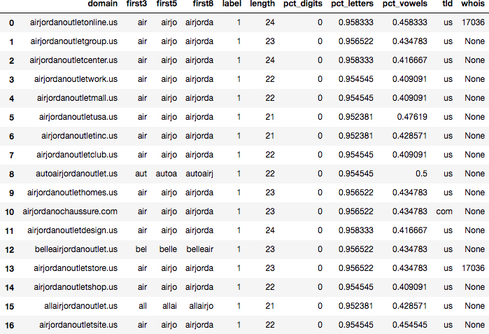
Figure 6-2. Domains with the 7-gram “jordano”
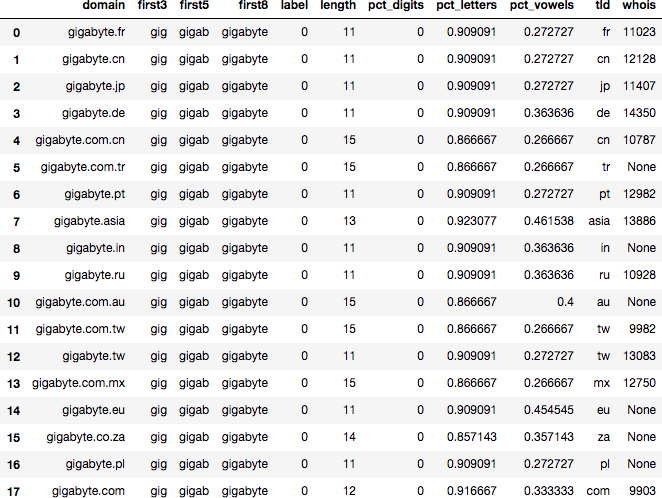
Figure 6-3. Domains with the 7-gram “gabyte”
Expanding the 5 numerical and 4 categorical features as just described gives a total of 65 features. For example, the “whois” domain-level feature (which gives the age of the domain in days) produces the cluster-level features shown in Figure 6-4.

Figure 6-4. Examples of cluster-level features for “whois”
Whereas the “top-level domain” feature produces the features in Figure 6-5.
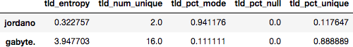
Figure 6-5. Examples of cluster-level features for “top-level domain”
From these two examples, we expect the fact that most whois results return null for the bad domains and return a wide range of results for the good domains to be a distinguishing feature. We also expect that high diversity of top-level domains indicates a good cluster.
Classification
Now let’s attempt to put this intuition into practice by training a classifier. We will use a random forest classifier, which is a nonlinear classifier that tends to be effective “out of the box” with little tuning. We downsample the good clusters in the training set in order not to overwhelm the classifier; however, we leave the test set unbiased so that we get an accurate calculation of precision and recall:
fromsklearn.metricsimportroc_auc_score,roc_curve,precision_recall_curvefromsklearn.model_selectionimporttrain_test_splitfromsklearn.ensembleimportRandomForestClassifierfromrandomimportrandomimportmatplotlib.pyplotasplt# Add a random entry to each row, to be used for samplingR=[random()foriinrange(len(ngram_cluster_features))]ngram_cluster_features['rand']=R# Split into 2/3 train, 1/3 test, and downsample good clusterstrain,test=train_test_split(ngram_cluster_features.fillna(value=0),test_size=0.33)sample_factor=0.2sampled_train=train[(train.label==1)|(train.label==0)&(train.rand<sample_factor)]# Fit and predictfeatures=sampled_train[sampled_train.columns.difference(['label','rand','score'])]labels=sampled_train.labelclf=RandomForestClassifier(n_estimators=20)clf.fit(features,labels)probs=clf.predict_proba(test[train.columns.difference(['label','rand','score'])])# Compute and plot P-R curveprecision,recall,thresholds=precision_recall_curve(test.label,probs[:,1])plt.step(recall,precision,color='b',alpha=0.2,where='post')plt.fill_between(recall,precision,step='post',alpha=0.2,color='b')plt.xlabel('Recall')plt.ylabel('Precision')plt.ylim([0.0,1.05])plt.xlim([0.0,1.0])plt.title('Precision-Recall curve for 7-gram groupings')plt.show()# Find threshold for 95% precisionm=min([iforiinrange(len(precision))ifprecision[i]>0.95])p,r,t=precision[m],recall[m],thresholds[m](p,r,t)
From this calculation and the precision-recall curve for this classifier in Figure 6-6, we see that we can achieve 61% recall and 95% precision on clusters at a threshold of 0.75 (i.e., 15 of the 20 trees in our forest classify the cluster as bad).

Figure 6-6. Precision-recall curve for 7-gram groupings for spam domain classification
But this calculation is at the cluster level—what is our precision and recall on the individual domain level? For example, if false positives tended to be larger clusters on average than true positives, our precision on individual domains would be less than on clusters.
We can work out the item-level precision and recall as follows:
# Compute item-level precision/recallpos=(test.score*test['count'])neg=(1-test.score)*(test['count'])tp=sum(pos[test.label>=t])fp=sum(neg[test.label>=t])tn=sum(neg[test.label<t])fn=sum(pos[test.label<t])item_precision=1.0*tp/(tp+fp)item_recall=1.0*tp/(tp+fn)
In this example, we find that precision drops slightly to 92%, but recall goes all the way down to 21%. This result makes sense intuitively, given that many bad domains in our dataset are not part of clusters and must thus be detected via some other means.
Further Directions in Clustering
In the previous example, we demonstrated how to use various algorithms to generate clusters in our example dataset, and then how to programmatically determine which clusters are abusive from the data. When implementing your own clustering system, there are several directions in which you could extend this example:
-
Experiment with different clustering methods, such as those discussed in Chapter 2.
-
Experiment with different classifiers and classifier parameters.
-
Add new features at the item level.
-
Add new aggregate features at the cluster level.
-
Sample the data so that “semi-good” clusters (i.e., those whose proportion of bad items is near the threshold for declaring the cluster bad) have less influence on the outcome.
-
Give extra weight to items appearing in multiple good or bad clusters.
-
Add a second classifier to detect false positive items within a cluster (e.g., if 19 of 20 items in the cluster are bad but the 20th is obviously good, can we detect the good item automatically?).
As in many other aspects of security, the best intuition for further work will come from looking at the data: What are the trends you are missing? What features can you use to identify classifier mistakes? In what way are false positives/false negatives similar to each other? When you can answer these questions qualitatively, you can use the framework of this chapter to improve your algorithmic solution to the problem.
Conclusion
The consumer web (and associated apps) provides a vast array of surfaces that bad actors can use to monetize. In most cases the attack will require one or many accounts, so preventing attackers from gaining access to accounts can stop many different kinds of attacks. In this chapter, we discussed ways to prevent account takeover and fake account creation, which are the two ways bad guys can get access to the accounts they need. We also considered ways to detect financial fraud and automation, which are two of the common techniques used to attack almost any product.
Machine learning for abuse problems comes with its own set of challenges: getting ground truth data is difficult, and models must achieve a delicate balance between finding what is already known and uncovering new attack techniques. We have considered some of the pitfalls of machine learning for abuse and offered some suggestions to mitigate them.
Although supervised learning is very powerful for addressing abuse problems, in many cases clustering techniques can be used to address attacks at scale. When combined with supervised learning, these techniques might allow you to detect and stop large attacks very quickly. We demonstrated some clustering techniques through a worked example of classifying spammy domain names.
To this point our discussion has been somewhat academic: collect certain signals, implement certain algorithms, and detect the bad guys. In real life, however, things aren’t so neat. Chapter 7 focuses on the issues that come up when translating the ideas discussed so far into a real-world system.
1 Anupam Das et al., “The Tangled Web of Password Reuse,” Proceedings of the 21st Annual Network and Distributed System Security Symposium (2014).
2 Because best practice is for passwords to be hashed and salted, a secure site will not know the distribution of its own passwords. Popularity rank can be estimated using publicly leaked lists.
3 For an alternative smoothing technique using the fact that IP addresses reside in hierarchies (e.g., IP → ISP → Country), see D. Freeman et al., “Who Are You? A Statistical Approach to Measuring User Authenticity,” Proceedings of the 23rd Annual Network and Distributed System Security Symposium (2016).
4 Michael Noll gives a good implementation of a rolling counter algorithm in his blog.
5 This equivalence breaks down if you allow or encourage automated activity; for example, if you have APIs that can be regularly polled for data.
6 Grégoire Jacob et al., “PUBCRAWL: Protecting Users and Businesses from CRAWLers,” Proceedings of the 21st USENIX Security Symposium (2012).
7 Gang Wang et al., “You Are How You Click: Clickstream Analysis for Sybil Detection,” Proceedings of the 22nd USENIX Security Symposium (2013): 241–255.
8 Elie Bursztein et al., “Picasso: Lightweight Device Class Fingerprinting for Web Clients,” Proceedings of the 6th Workshop on Security and Privacy in Smartphones and Mobile Devices (2016): 93–102.
9 For example, the crawler-user-agents repository.
10 We will call bad requests “positive” and good requests “negative.” Whether to label bad requests as 0 or 1 is left to you—just be consistent!
11 For details, see Burr Settles, “Active Learning Literature Survey,” Computer Sciences Technical Report 1648, University of Wisconsin–Madison (2010).
12 “No resource should be infinite” is a good principle here. In practice, this means that there should be global backstops on all types of activity per account—logins, messages, transactions, and even pageviews.
13 This is a categorical feature, as opposed to the n-gram feature, which produces lists of unequal length.
14 You might wonder how the sum of TP domains and FP domains can be less than 10 times the number of bad clusters if the minimum cluster size is 10; the answer is that some domains can appear in multiple clusters, and we deduplicate when computing the TP/FP stats.
15 This module contains our implementation of the MinHash algorithm and can be found at https://github.com/oreilly-mlsec/book-resources/tree/master/chapter6.