Chapter 2. Classifying and Clustering
In this chapter, we discuss the most useful machine learning techniques for security applications. After covering some of the basic principles of machine learning, we offer up a toolbox of machine learning algorithms that you can choose from when approaching any given security problem. We have tried to include enough detail about each technique so that you can know when and how to use it, but we do not attempt to cover all the nuances and complexities of the algorithms.
This chapter has more mathematical detail than the rest of the book; if you want to skip the details and begin trying out the techniques, we recommend you read the sections “Machine Learning in Practice: A Worked Example” and “Practical Considerations in Classification” and then look at a few of the most popular supervised and unsupervised algorithms: logistic regression, decision trees and forests, and k-means clustering.
Machine Learning: Problems and Approaches
Suppose that you are in charge of computer security for your company. You install firewalls, hold phishing training, ensure secure coding practices, and much more. But at the end of the day, all your CEO cares about is that you don’t have a breach. So, you take it upon yourself to build systems that can detect and block malicious traffic to any attack surface. Ultimately, these systems must decide the following:
-
For every file sent through the network, does it contain malware?
-
For every login attempt, has someone’s password been compromised?
-
For every email received, is it a phishing attempt?
-
For every request to your servers, is it a denial-of-service (DoS) attack?
-
For every outbound request from your network, is it a bot calling its command-and-control server?
These tasks are all classification tasks—binary decisions about the nature of the observed event.
Your job can thus be rephrased as follows:
- Classify all events in your network as malicious or legitimate.
When phrased in this manner, the task seems almost hopeless; how are you supposed to classify all traffic? But not to fear! You have a secret weapon: data.
Specifically, you have historical logs of binary files, login attempts, emails received, and inbound and outbound requests. In some cases, you might even know of attacks in the past and be able to associate these attacks with the corresponding events in your logs. Now, to begin solving your problem, you look for patterns in the past data that seem to indicate malicious attacks. For example, you observe that when a single IP address is making more than 20 requests per second to your servers over a period of 5 minutes, it’s probably a DoS attack. (Maybe your servers went down under such a load in the past.)
After you have found patterns in the data, the next step is to encode these patterns as an algorithm—that is, a function that takes as input data about whatever you’re trying to classify and outputs a binary response: “malicious” or “legitimate.” In our example, this algorithm would be very simple:1 it takes as input the number of requests from an IP address over the 5 minutes prior to the request, and outputs “legitimate” if the number is less than 6,000 and “malicious” if it is greater than 6,000.
At this point, you have learned from the data and created an algorithm to block bad traffic. Congratulations! But there should be something nagging at you: what’s special about the number 20? Why isn’t the limit 19 or 21? Or 19.77? Ideally you should have some principled way of determining which one of these options, or in fact which real number, is best. And if you use an algorithm to scan historical data and find the best classification rule according to some mathematical definition of “best,” this process is called machine learning.
More generally, machine learning is the process of using historical data to create a prediction algorithm for future data. The task we just considered was one of classification: determine which class a new data point (the request) falls into. Classification can be binary, as we just saw, in which there are only two classes, or multiclass; for example, if you want to determine whether a piece of malware is ransomware, a keylogger, or a remote access trojan.
Machine learning can also be used to solve regression problems, in which we try to predict the value of a real-number variable. For example, you might want to predict the number of phishing emails an employee receives in a given month, given data about their position, access privileges, tenure in the company, security hygiene score, and so on. Regression problems for which the inputs have a time dimension are sometimes called time series analysis; for example, predicting the value of a stock tomorrow given its past performance, or the number of account sign-ins from the Seattle office given a known history. Anomaly detection is a layer on top of regression: it refers to the problem of determining when an observed value is sufficiently different from a predicted value to indicate that something unusual is going on.
Machine learning is also used to solve clustering problems: given a bunch of data points, which ones are similar to one another? For example, if you are trying to analyze a large dataset of internet traffic to your site, you might want to know which requests group together. Some clusters might be botnets, some might be mobile providers, and some might be legitimate users.
Machine learning can be supervised, in which case you have labels on historical data and you are trying to predict labels on future data. For example, given a large corpus of emails labeled as spam or ham, you can train a spam classifier that tries to predict whether a new incoming message is spam. Alternatively, machine learning can be unsupervised, in which case you have no labels on the historical data; you might not even know what the labels are that you’re trying to predict, for example if you have an unknown number of botnets attacking your network that you want to disambiguate from one another. Classification and regression tasks are examples of supervised learning, and clustering is a typical form of unsupervised learning.
Machine Learning in Practice: A Worked Example
As we said earlier, machine learning is the process of using historical data to come up with a prediction algorithm for previously unseen data. Let’s examine how this process works, using a simple dataset as an example. The dataset that we are using is transaction data for online purchases collected from an ecommerce retailer.2 The dataset contains 39,221 transactions, each comprising 5 properties that can be used to describe the transaction, as well as a binary “label” indicating whether this transaction is an instance of fraud—“1” if fraudulent, and “0” if not. The comma-separated values (CSV) format that this data is in is a standard way of representing data for analytics. Observing that the first row in the file indicates the names for each positional value in each subsequent line, let’s consider what each value means by examining a randomly selected row of data:
accountAgeDays,numItems,localTime,paymentMethod,paymentMethodAgeDays,label
...
196, 1, 4.962055, creditcard, 5.10625, 0
Putting this in a more human-readable form:
accountAgeDays:       196
numItems:             1
localTime:            4.962055
paymentMethod:        creditcard
paymentMethodAgeDays: 5.10625
label:                0
We see that this transaction was made through a user account that was created 196 days ago (accountAgeDays), and that the user purchased 1 item (numItems) at around 4:58 AM in the consumer’s local time (localTime). Payment was made through credit card (paymentMethod), and this method of payment was added about 5 days before the transaction (paymentMethodAgeDays). The label is 0, which indicates that this transaction is not fraudulent.
Now, you might ask how we came to learn that a certain transaction was fraudulent. If someone made an unauthorized transaction using your credit card, assuming that you were vigilant, you would file a chargeback for this transaction, indicating that the transaction was not made by you and you want to get your money back. Similar processes exist for payments made through other payment methods, such as PayPal or store credit. The chargeback is a strong and clear indication that the transaction is fraudulent, allowing us to collect data about fraudulent transactions.
However, the reason we can’t use chargeback data in real time is that merchants receive chargeback details many months after the transaction has gone through—after they have shipped the items out to the attackers, never to be seen again. Typically, the retailer absorbs all losses in situations like this, which could translate to potentially enormous losses in revenue. This financial loss could be mitigated if we had a way to predict how likely a transaction is to be fraudulent before we ship the items out. Now, we could examine the data and come up with some rules, such as “If the payment method was added in the last day and the number of items is at least 10, the transaction is fraudulent.” But such a rule might have too many false positives. How can we use data to find the best prediction algorithm? This is what machine learning does.
Each property of a transaction is called a feature in machine learning parlance. What we want to achieve is to have a machine learning algorithm learn how to identify a fraudulent transaction from the five features in our dataset. Because the dataset contains a label for what we are aiming to predict, we call this a “labeled dataset” and can perform supervised learning on it. (If there had been no label, we could only have performed semi-supervised learning or unsupervised learning.) The ideal fraud detection system will take in features of a transaction and return a probability score for how likely this transaction is to be fraudulent. Let’s see how we can create a prototype system by using machine learning.
Similar to how we approached the spam classification problem in Chapter 1, we’ll take advantage of the functionality in the Python machine learning library scikit-learn. In addition, we’ll use Pandas, a popular data analysis library for Python, to perform some lightweight data wrangling. First, we’ll use the pandas.read_csv() utility to read the dataset in the CSV file:
importpandasaspddf=pd.read_csv('ch1/payment_fraud.csv')
Notice that the result of read_csv() is stored into the variable df, short for DataFrame. A DataFrame is a Pandas data structure that represents datasets in a two-dimensional table-like form, allowing for operations to be applied on rows or columns. DataFrame objects allow you to perform a plethora of manipulations on the data, but we will not dive into the specifics here.3 Let’s use the DataFrame.sample() function to retrieve a snippet of three rows from df:
df.sample(3)
| accountAgeDays | numItems | localTime | paymentMethod | paymentMethodAgeDays | label | |
|---|---|---|---|---|---|---|
31442 |
2000 |
1 |
4.748314 |
storecredit |
0.000000 |
0 |
27232 |
1 |
1 |
4.886641 |
storecredit |
0.000000 |
1 |
8687 |
878 |
1 |
4.921349 |
paypal |
0.000000 |
0 |
This command returns a tabular view of three random rows. The left column indicates the numerical index of each selected row, and the top row indicates the name of each column. Note that one column stands out because it is of non-numerical type: paymentMethod. There are three possible values that this feature takes on in our dataset: creditcard, paypal, and storecredit. This feature is called a categorical variable because it takes on a value indicating the category it belongs to. Many machine learning algorithms require all features to be numeric.4 We can use pandas.get_dummies() to convert variables from categorical to numeric:5
df=pd.get_dummies(df,columns=['paymentMethod'])
Upon inspection of the new DataFrame object, we notice that three new columns have been added to the table—paymentMethod_creditcard, paymentMethod_paypal, and paymentMethod_storecredit:
df.sample(3)
| accountAgeDays | … | paymentMethod_creditcard | paymentMethod_paypal | paymentMethod_storecredit | |
|---|---|---|---|---|---|
23393 |
57 |
… |
1 |
0 |
0 |
3355 |
1,366 |
… |
0 |
1 |
0 |
34248 |
19 |
… |
1 |
0 |
0 |
Each of these features is a binary feature (i.e., they take on a value of either 0 or 1), and each row has exactly one of these features set to 1, hence the name of this method of categorical variable encoding: one-hot encoding. These variables are called dummy variables in statistics terminology.
Now, we can divide the dataset into training and test sets (as we did in Chapter 1):
fromsklearn.model_selectionimporttrain_test_splitX_train,X_test,y_train,y_test=train_test_split(df.drop('label',axis=1),df['label'],test_size=0.33,random_state=17)
The sklearn.model_selection.train_test_split() function helps us split our dataset into training and test sets. Notice that in the first argument to the function, we passed in df.drop('label', axis=1). This will be split into X_train and X_test to the ratio of 0.67:0.33 because we passed in test_size=0.33, which means that we want two-thirds of the dataset to be used for training the machine learning algorithm, and the remaining third, the test set, to be used to see how well the algorithm performs. We are dropping the label column from X before splitting it into X_train and X_test, and passing in the label column as y—df['label']. The labels will then be split in the same ratio into y_train and y_test.
Now let’s apply a standard supervised learning algorithm, logistic regression, to this data:
fromsklearn.linear_modelimportLogisticRegressionclf=LogisticRegression()clf.fit(X_train,y_train)
In the first line, we import the sklearn.linear_model.LogisticRegression class. Then, in the second line, we initialize the LogisticRegression object by invoking the constructor. In the third line, we feed X_train and y_train (i.e., the training set) into the fit() function, resulting in a trained classifier model, which is stored in the clf object. This classifier has taken the training data and used logistic regression (which we elaborate on further in the next section) to distill some generalizations about fraudulent and nonfraudulent transactions into a model.
To make predictions using this model, all we need to do now is to pass some unlabeled features into this classifier object’s predict() function:
y_pred=clf.predict(X_test)
Inspecting y_pred, we can see the label predictions made for each row in X_test. Note that at training time the classifier did not have any access to y_test at all; the predictions made, contained in y_pred, are thus purely a result of the generalizations learned from the training set. We use the sklearn.metrics.accuracy_score() function (that we also used in Chapter 1) to get a feel of how good these predictions are:
fromsklearn.metricsimportaccuracy_score(accuracy_score(y_pred,y_test))>0.99992273816
A 99.992% accuracy is pretty good! However, we discussed in Chapter 1 that the accuracy score can often be a misleading oversimplification and is quite a bad metric for evaluating results like this. Let’s generate a confusion matrix, instead:
fromsklearn.metricsimportconfusion_matrix(confusion_matrix(y_test,y_pred))
| 0 | Predicted NOT FRAUD | Predicted FRAUD |
|---|---|---|
Actual NOT FRAUD |
12,753 |
0 |
Actual FRAUD |
1 |
189 |
There appears to only be a single misclassification in the entire test set. 189 transactions are correctly flagged as fraud, and there is 1 false negative in which the fraudulent transaction was not detected. There are zero false positives.
As a recap, here is the entire piece of code that we used to train and test our logistic regression payment fraud detection model:6
importpandasaspdfromsklearn.model_selectionimporttrain_test_splitfromsklearn.linear_modelimportLogisticRegressionfromsklearn.metricsimportaccuracy_score,confusion_matrix# Read in the data from the CSV filedf=pd.read_csv('ch1/payment_fraud.csv')# Convert categorical feature into dummy variables with one-hot encodingdf=pd.get_dummies(df,columns=['paymentMethod'])# Split dataset into training and test setsX_train,X_test,y_train,y_test=train_test_split(df.drop('label',axis=1),df['label'],test_size=0.33,random_state=17)# Initialize and train classifier modelclf=LogisticRegression().fit(X_train,y_train)# Make predictions on test sety_pred=clf.predict(X_test)# Compare test set predictions with ground truth labels(accuracy_score(y_pred,y_test))(confusion_matrix(y_test,y_pred))
We can apply this model to any given incoming transaction and get a probability score for how likely this transaction is to be fraudulent:
clf.predict_proba(df_real)# Array that represents the probability of the transaction# having a label of 0 (in position 0) or 1 (in position 1)>[[9.99999994e-015.87025707e-09]]
Taking df_real to be a DataFrame that contains a single row representing an incoming transaction received by the online retailer, the classifier predicts that this transaction is 99.9999994% likely to not be fraudulent (remember that y = 0 means not fraudulent).
You might have noticed that all the work of machine learning—i.e., the part where we learn the prediction algorithm—has been abstracted out into the single scikit-learn API call, LogisticRegression.fit(). So, what actually goes on in this black box that allows this model to learn how to predict fraudulent transactions? We will now open up the box and find out.
Training Algorithms to Learn
At its core, a machine learning algorithm takes in a training dataset and outputs a model. The model is an algorithm that takes in new data points in the same form as the training data and outputs a prediction. All machine learning algorithms are defined by three interdependent components:
-
A model family, which describes the universe of models from which we can choose
-
A loss function, which allows us to quantitatively compare different models
-
An optimization procedure, which allows us to choose the best model in the family
Let’s now consider each of these components.
Model Families
Recall that we expressed our fraud dataset in terms of seven numerical features: four features from the raw data and three from the one-hot encoding of the payment method. We can thus think of each transaction as a point in a seven-dimensional real vector space, and our goal is to divide up the space into areas of fraud and nonfraud transactions. The “model” output by our machine learning algorithm is a description of this division of the vector space.
In theory, the division of our vector space into fraud and nonfraud areas can be infinitely complex; in practice, most algorithms produce a decision boundary, which is a surface in the vector space.7 One side of the decision boundary consists of the points labeled as fraud, and the other side consists of the points labeled as nonfraud. The boundary can be as simple as a line (or hyperplane in higher dimensions) or as complex as a union of nonlinear disconnected regions. Figure 2-1 presents some examples.

Figure 2-1. Examples of two-dimensional spaces divided by a decision boundary
If we want to be more granular, instead of mapping each point in the vector space to either “fraud” or “nonfraud,” we can map each point to a probability of fraud. In this case our machine learning algorithm outputs a function that assigns each point in the vector space a value between 0 and 1, to be interpreted in our example as the probability of fraud.
Any given machine learning algorithm restricts itself to finding a certain type of decision boundary or probability function that can be described by a finite number of model parameters. The simplest decision boundary is a linear decision boundary—that is, a hyperplane in the vector space. An oriented hyperplane H in an n-dimensional vector space can be described by an n-dimensional vector orthogonal to the hyperplane, plus another vector indicating how far the hyperplane is from the origin:
This description allows us to divide the vector space in two; to assign probabilities we want to look at the distance of the point from the hyperplane H. We can thus compute a real-valued “score”:
where we have let . Our model to compute the score can thus be described by n + 1 model parameters: n parameters to describe the vector , and one “offset” parameter b. To turn the score into a classification, we simply choose a threshold t above which all scores indicate fraud, and below which all scores indicate nonfraud.
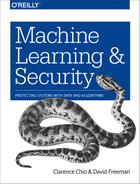
If we want to map the real-valued score to a probability, we must apply a function that maps the real numbers to the interval [0,1]. The standard function to apply is known as the logistic function or sigmoid function,8 as illustrated in Figure 2-2. It is formulated as:
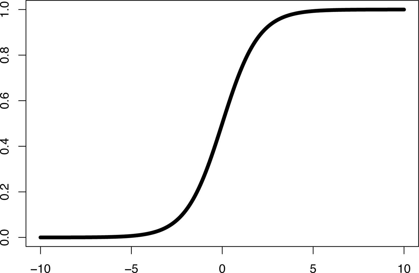
Figure 2-2. The sigmoid function
The output of the logistic function can be interpreted as a probability, allowing us to define the likelihood of the dependent variable taking on a particular value given some input feature vector .
Loss Functions
Now that we have restricted our choice of prediction algorithms to a certain parametrized family, we must choose the best one for the given training data. How do we know when we have found the best algorithm? We define the best algorithm to be one that optimizes some quantity computed from the data. This quantity is called an objective function. In the case of machine learning, the objective function is also known as a cost function or loss function, because it measures the “cost” of wrong predictions or the “loss” associated with them.
Mathematically, a loss function is a function that maps a set of pairs of (predicted label, truth label) to a real number. The goal of a machine learning algorithm is to find the model parameters that produce predicted labels for the training set that minimize the loss function.
In regression problems, for which the prediction algorithm outputs a real number instead of a label, the standard loss function is the sum of squared errors. If is the true value and is the predicted value, the loss function is as follows:
We can use this loss function for classification problems as well, where is either 0 or 1, and is the probability estimate output by the algorithm.
For logistic regression, we use negative log likelihood as the loss function. The likelihood of a set of probability predictions for a given set of ground truth labels is defined to be the probability that these truth labels would have arisen if sampled from a set of binomial distributions according to the probabilities . Concretely, if the truth label is 0, the likelihood of 0 is —the probability that 0 would have been sampled from a binomial distribution with mean . If the truth label is 1, the likelihood is .
The likelihood of the entire set of predictions is the product of the individual likelihoods:
The goal of logistic regression is to find parameters that produce probabilities that maximize the likelihood.
To make computations easier, and, in particular, because most optimization methods require computing derivatives of the loss function, we take the negative log of the likelihood. As maximizing the likelihood is equivalent to minimizing the negative log likelihood, we call negative log likelihood the loss function:
Here we have used the fact that is always 0 or 1 to combine the two products into a single term.
Optimization
The last step in the machine learning procedure is to search for the optimal set of parameters that minimizes the loss function. To carry out this search we use an optimization algorithm. There may be many different optimization algorithms available to you when fitting your machine learning model.9 Most scikit-learn estimators (e.g., LogisticRegression) allow you to specify the numerical solver to use, but what are the differences between the different options, and how do you go about selecting one?
The job of an optimization algorithm is to minimize (or maximize) an objective function. In the case of machine learning, the objective function is expressed in terms of the model’s learnable parameters ( and b in the previous example), and the goal is to find the values of and b that optimize the objective function.
Optimization algorithms mainly come in two different flavors:
- First-order algorithms
-
These algorithms optimize the objective function using the first derivatives of the function with respect to the learnable parameters. Gradient descent methods are the most popular types of first-order optimization algorithms; we can use them to find the inputs to a function that give the minimum (or maximum) value. Computing the gradient of a function (i.e., the partial derivatives with respect to each variable) allows us to determine the instantaneous direction that the parameters need to move in order to achieve a more optimal outcome.
- Second-order algorithms
-
As the name suggests, these algorithms use the second derivatives to optimize the objective function. Second-order algorithms will not fall victim to paths of slow convergence. For example, second-order algorithms are good at detecting saddle points, whereas first-order algorithms are likely to become stuck at these points. However, second-order methods are often slower and more expensive to compute.
First-order methods tend to be much more frequently used because of their relative efficiency. Picking a suitable optimization algorithm depends on the size of the dataset, the nature of the cost function, the type of learning problem, and speed/resource requirements for the operation. In addition, some regularization techniques can also have compatibility issues with certain types of optimizers. First-order algorithms include the following:
-
LIBLINEAR10 is the default solver for the linear estimators in scikit-learn. This algorithm tends to not do well on larger datasets; as suggested by the scikit-learn documentation, the Stochastic Average Gradient (SAG) or SAGA (improvement to SAG) methods work better for large datasets.11
Different optimization algorithms deal with multiclass classification differently. LIBLINEAR works only on binary classification. For it to work in a multiclass scenario, it has to use the one-versus-rest scheme; we discuss this scheme more fully in Chapter 5.
-
Stochastic Gradient Descent (SGD) is a very simple and efficient algorithm for optimization that performs a parameter update for each separate training example. The stochastic nature of the gradient descent means that the algorithm is more likely to discover new and possibly better local minima as compared to standard gradient descent. However, it typically results in high-variance oscillations, which can result in a delay in convergence. This can be solved with a decreasing learning rate (i.e., exponentially decrease the learning rate) that results in smaller fluctuations as the algorithm approaches convergence.
The technique called momentum also helps accelerate SGD convergence by navigating the optimization movement only in the relevant directions and softening any movement in irrelevant directions, which stabilizes SGD.
-
Optimization algorithms such as AdaGrad, AdaDelta, and Adam (Adaptive Moment Estimation) allow for separate and adaptive learning rates for each parameter that solve some problems in the other simpler gradient descent algorithms.
-
When your training dataset is large, you will need to use a distributed optimization algorithm. One popular algorithm is the Alternating Direction Method of Multipliers (ADMM).12
Example: Gradient descent
To conclude this section, we go briefly into the details of gradient descent, a powerful optimization algorithm that has been applied to many different machine learning problems.
The standard algorithm for gradient descent is as follows:
-
Select random starting parameters for the machine learning model. In the case of a linear model, this means selecting a random normal vector and offset , which results in a random hyperplane in n-dimensional space.
-
Compute the value of the gradient of the loss function for this model at the point described by these parameters.
-
Change the model parameters in the direction of greatest gradient decrease by a certain small magnitude, typically referred to as the α or learning rate.
-
Iterate: repeat steps 2 and 3 until convergence or a satisfactory optimization result is attained.
Figure 2-3 illustrates the intermediate results of a gradient descent optimization process of a linear regression. At zero iterations, observe that the regression line, formed with the randomly chosen parameters, does not fit the dataset at all. As you can imagine, the value of the sum-of-squares cost function is quite large at this point. At three iterations, notice that the regression line has very quickly moved to a more sensible position. Between 5 and 20 iterations the regression line slowly adjusts itself to more optimal positions where the cost function is minimized. If performing any more iterations doesn’t decrease the cost function significantly, we can say that the optimization has converged, and we have the final learned parameters for the trained model.

Figure 2-3. Regression line after a progressive number of iterations of gradient descent optimization (0, 3, 5, and 20 iterations of gradient descent, shown at the upper left, upper right, lower left, and lower right, respectively)
Which optimization algorithm?
As with many things in data science, no optimization algorithm is one-size-fits-all, and there are no clear rules for which algorithm definitely performs better for certain types of problems. A certain amount of trial-and-error experimentation is often needed to find an algorithm that suits your requirements and meets your needs. There are many considerations other than convergence or speed that you should take into account when selecting an optimizer. Starting with the default or the most sensible option and iterating when you see clues for improvements is generally a good strategy.
Supervised Classification Algorithms
Now that we know how machine learning algorithms work in principle, we will briefly describe some of the most popular supervised learning algorithms for classification.
Logistic Regression
Although we discussed logistic regression in some detail earlier, we go over its key properties here. Logistic regression takes as input numerical feature vectors and attempts to predict the log odds13 of each data point occurring; we can convert the log odds to probabilities by using the sigmoid function discussed earlier. In the log odds space, the decision boundary is linear, so increasing the value of a feature monotonically increases or decreases (depending on the sign of the coefficient) the score output by the model.
Logistic regression is one of the most popular algorithms in practice due to a number of properties: it can be trained very efficiently and in a distributed manner, it scales well to millions of features, it admits a concise description and fast scoring algorithm (a simple dot product), and it is explainable—each feature’s contribution to the final score can be computed.
However, there are a few important things to be aware of when considering logistic regression as a supervised learning technique:
-
Logistic regression assumes linearity of features (independent variables) and log odds, requiring that features are linearly related to the log odds. If this assumption is broken the model will perform poorly.
-
Features should have little to no multicollinearity;14 that is, independent variables should be truly independent from one another.
-
Logistic regression typically requires a larger sample size compared to other machine learning algorithms like linear regression. Maximum likelihood estimates (used in logistic regression) are less powerful than ordinary least squares (used in linear regression), which results in requiring more training samples to achieve the same statistical learning power.15
Decision Trees
Decision trees are very versatile supervised learning models that have the important property of being easy to interpret. A decision tree is, as its name suggests, a binary tree data structure that is used to make a decision. Trees are a very intuitive way of displaying and analyzing data and are popularly used even outside of the machine learning field. With the ability to predict both categorical values (classification trees) and real values (regression trees) as well as being able to take in numerical and categorical data without any normalization or dummy variable creation,16 it’s not difficult to see why they are a popular choice for machine learning.
Let’s see how a typical (top-down) learning decision tree is constructed:
-
Starting at the root of the tree, the full dataset is split based on a binary condition into two child subsets. For example, if the condition is “age ≥ 18,” all data points for which this condition is true go to the left child and all data points for which this condition is false go to the right child.
-
The child subsets are further recursively partitioned into smaller subsets based on other conditions. Splitting conditions are automatically selected at each step based on what condition best splits the set of items. There are a few common metrics by which the quality of a split is measured:
- Gini impurity
-
If samples in a subset were randomly labeled according to the distribution of labels in the set, the proportion of samples incorrectly labeled would be the Gini impurity. For example, if a subset were made up of 25% samples with label 0 (and 75% with label 1), assigning label 0 to a random 25% of all samples (and label 1 to the rest) would give 37.5% incorrect labels: 75% of the label-0 samples and 25% of the label-1 samples would be incorrect. A higher-quality decision tree split would split the set into subsets cleanly separated by their label, hence resulting in a lower Gini impurity; that is, the rate of misclassification would be low if most points in a set belong to the same class.
- Variance reduction
-
Often used in regression trees, where the dependent variable is continuous. Variance reduction is defined as the total reduction in a set’s variance as a result of the split into two subsets. The best split at a node in a decision tree would be the split that results in the greatest variance reduction.
- Information gain
-
Information gain is a measure of the purity of the subsets resulting from a split. It is calculated by subtracting the weighted sum of each decision tree child node’s entropy from the parent node’s entropy. The smaller the entropy of the children, the greater the information gain, hence the better the split.
-
There are a few different methods for determining when to stop splitting nodes:
-
When all leaves of the tree are pure—that is, all leaf nodes each only contain samples belonging to the same class—stop splitting.
-
When a branch of the tree has reached a certain predefined maximum depth, the branch stops being split.
-
When either of the child nodes will contain fewer than the minimum number of samples, the node will not be partitioned.
-
-
Ultimately the algorithm outputs a tree structure where each node represents a binary decision, the children of each node represent the two possible outcomes of that decision, and each leaf represents the classification of data points following the path from the root to that leaf. (For impure leaves, the decision is determined by majority vote of the training data samples at that leaf.)
An important quality of decision trees is the relative ease of explaining classification or regression results, since every prediction can be expressed in a series of Boolean conditions that trace a path from the root of the tree to a leaf node. For example, if a decision tree model predicted that a malware sample belongs to malware family A, we know it is because the binary was signed before 2015, does not hook into the window manager framework, does make multiple network calls out to Russian IP addresses, etc. Because each sample traverses at most the height of the binary tree (time complexity ), decision trees are also efficient to train and make predictions on. As a result, they perform favorably for large datasets.
Nevertheless, decision trees have some limitations:
-
Decision trees often suffer from the problem of overfitting, wherein trees are overly complex and don’t generalize well beyond the training set. Pruning is introduced as a regularization method to reduce the complexity of trees.
-
Decision trees are more inefficient at expressing some kinds of relationships than others. For example, Figures 2-5 and 2-6 present the minimal decision tree required to represent the AND, OR, and XOR relationships. Notice how XOR requires one more intermediate node and split to be appropriately represented, even in this simple example. For realistic datasets, this can quickly result in exploding model complexity.

Figure 2-5. Decision tree for A-AND-B → y=1 (left), A-OR-B → y=1 (right)
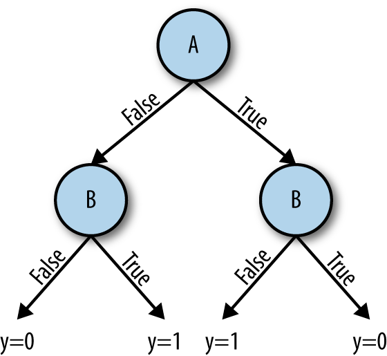
Figure 2-6. Decision tree for A-XOR-B → y=1 (bottom)
-
Decision trees tend to be less accurate and robust than other supervised learning techniques. Small changes to the training dataset can result in large changes to the tree, which in turn result in changes to model predictions. This means that decision trees (and most other related models) are unsuitable for use in online learning or incremental learning.
-
Split-quality metrics for categorical variables in decision trees are biased toward variables with more possible values; that is, splits on continuous variables or categorical variables with three or more categories will be chosen with a greater probability than binary variables.
-
Greedy training of decision trees (as it is almost always done) does not guarantee an optimal decision tree because locally optimal and not globally optimal decisions are made at each split point. In fact, the training of a globally optimal decision tree is an NP-complete problem.17
Decision Forests
An ensemble refers to a combination of multiple classifiers that creates a more complex, and often better performing, classifier. Combining decision trees into ensembles is a proved technique for creating high-quality classifiers. These ensembles are aptly named decision forests. The two most common types of forests used in practice are decision forests and gradient-boosted decision trees:
-
Random forests are formed by simple ensembling of multiple decision trees, typically ranging from tens to thousands of trees. After training each individual decision tree, overall random forest predictions are made by taking the statistical mode of individual tree predictions for classification trees (i.e., each tree “votes”), and the statistical mean of individual tree predictions for regression trees.
You might notice that simply having many decision trees in the forest will result in highly similar trees and a lot of repeated splits across different trees, especially for features that are strong predictors of the dependent variable. The random forest algorithm addresses this issue using the following training algorithm:
-
For the training of each individual tree, randomly draw a subset of N samples from the training dataset.
-
At each split point, we randomly select m features from the p available features, where ,18 and pick the optimal split point from these m features.19
-
Repeat step 2 until the individual tree is trained.
-
Repeat steps 1, 2, and 3 until all trees in the forest are trained.
Single decision trees tend to overfit to their training sets, and random forests mitigate this effect by taking the average of multiple decision trees, which usually improves model performance. In addition, because each tree in the random forest can be trained independently of all other trees, it is straightforward to parallelize the training algorithm and therefore random forests are very efficient to train. However, the increased complexity of random forests can make them much more storage intensive, and it is much harder to explain predictions than with single decision trees.
-
-
Gradient-boosted decision trees (GBDTs) make use of smarter combinations of individual decision tree predictions to result in better overall predictions. In gradient boosting, multiple weak learners are selectively combined by performing gradient descent optimization on the loss function to result in a much stronger learning model.
The basic technique of gradient boosting is to add individual trees to the forest one at a time, using a gradient descent procedure to minimize the loss when adding trees. Addition of more trees to the forest stops either when a fixed limit is hit, when validation set loss reaches an acceptable level, or when adding more trees no longer improves this loss.
Several improvements to basic GBDTs have been made to result in better performing, better generalizing, and more efficient models. Let’s look at a handful of them:
-
Gradient boosting requires weak learners. Placing artificial constraints on trees, such as limits on tree depth, number of nodes per tree, or minimum number of samples per node, can help constrain these trees without overly diminishing their learning ability.
-
It can happen that the decision trees added early on in the additive training of gradient-boosted ensembles contribute much more to the overall prediction than the trees added later in the process. This situation results in an imbalanced model that limits the benefits of ensembling. To solve this problem, the contribution of each tree is weighted to slow down the learning process, using a technique called shrinkage, to reduce the influence of individual trees and allow future trees to further improve the model.
-
We can combine the stochasticity of random forests with gradient boosting by subsampling the dataset before creating a tree and subsampling the features before creating a split.
-
We can use standard and popular regularization techniques such as and regularization to smooth final learned weights to further avoid overfitting.
XGBoost20 is a popular GBDT flavor that achieves state-of-the-art results while scaling well to large datasets. As the algorithm that was responsible for many winning submissions to machine learning competitions, it garnered the attention of the machine learning community and has become the decision forest algorithm of choice for many practitioners. Nevertheless, GBDTs are more prone to overfitting than random forests, and also more difficult to parallelize because they use additive training, which relies on the results of a given tree to update gradients for the subsequent tree. We can mitigate overfitting of GBDTs by using shrinkage, and we can parallelize training within a single tree instead of across multiple trees.
-
Support Vector Machines
Like logistic regression, a support vector machine (SVM) is (in its simplest form) a linear classifier, which means that it produces a hyperplane in a vector space that attempts to separate the two classes in the dataset. The difference between logistic regression and SVMs is the loss function. Logistic regression uses a log-likelihood function that penalizes all points proportionally to the error in the probability estimate, even those on the correct side of the hyperplane. An SVM, on the other hand, uses a hinge loss, which penalizes only those points on the wrong side of the hyperplane or very near it on the correct side.
More specifically, the SVM classifier attempts to find the maximum-margin hyperplane separating the two classes, where “margin” indicates the distance from the separating plane to the closest data points on each side. For the case in which the data is not linearly separable, points within the margin are penalized proportionately to their distance from the margin. Figure 2-7 shows a concrete example: the two classes are represented by white and black points, respectively. The solid line is the separating plane and the dashed lines are the margins. The square points are the support vectors; that is, those that provide nonzero contribution to the loss function. This loss function is expressed mathematically as:
where is the margin, is the distance from the ith support vector to the margin, and C is a model hyperparameter that determines the relative contribution of the two terms.
Figure 2-7. Classification boundary (dark line) and margins (dashed lines) for linear SVM separating two classes (black and white points); squares represent support vectors
To classify a new data point x, we simply determine which side of the plane x falls on. If we want to get a real-valued score we can compute the distance from x to the separating plane and then apply a sigmoid to map to [0,1].
The real power of SVMs comes from the kernel trick, which is a mathematical transformation that takes a linear decision boundary and produces a nonlinear boundary. At a high level, a kernel transforms one vector space, , to another space, . Mathematically, the kernel is a function on defined by , and each is mapped to the function ; is the space spanned by all such functions. For example, we can recover the linear SVM by defining K to be the usual dot product .
If the kernel is nonlinear, a linear classifier in will produce a nonlinear classifier in . The most popular choice is the radial basis function . Even though we omit the mathematical details here,21 you can think of an SVM with the RBF kernel as producing a sort of smoothed linear combination of spheres around each point x, where the inside of each sphere is classified the same as x, and the outside is assigned the opposite class. The parameter determines the radius of these spheres; i.e., how close to each point you need to be in order to be classified like that point. The parameter C determines the “smoothing”; a large value of C will lead to the classifier consisting of a union of spheres, while a small value will yield a wigglier boundary influenced somewhat by each sphere. We can therefore see that too large a value of C will produce a model that overfits the training data, whereas too small a value will give a poor classifier in terms of accuracy. (Note that is unique to the RBF kernel, whereas C exhibits the same properties for any kernel, including the linear SVM. Optimal values of these parameters are usually found using grid search.)
SVMs have shown very good performance in practice, especially in high-dimensional spaces, and the fact that they can be described in terms of support vectors leads to efficient implementations for scoring new data points. However, the complexity of training a kernelized SVM grows quadratically with the number of training samples, so that for training set sizes beyond a few million, kernels are rarely used and the decision boundary is linear. Another disadvantage is that the scores output by SVMs are not interpretable as probabilities; converting scores to probabilities requires additional computation and cross-validation, for example using Platt scaling or isotonic regression. The scikit-learn documentation has further details.
Naive Bayes
The Naive Bayes classifier is one of the oldest statistical classifiers. The classifier is called “naive” because it makes a very strong statistical assumption, namely that features are chosen independently from some (unknown) distribution. This assumption never actually holds in real life. For example, consider a spam classifier for which the features are the words in the message. The Naive Bayes assumption posits that a spam message is composed by sampling words independently, where each word w has a probability of being sampled, and similarly for good messages. This assumption is clearly ludicrous; for one thing, it completely ignores word ordering. Yet despite the fact that the assumption doesn’t hold, Naive Bayes classifiers have been shown to be quite effective for problems such as spam classification.
The main idea behind Naive Bayes is as follows: given a data point with feature set , we want to determine the probability that the label Y for this point is the class C. In Equation 2-1, this concept is expressed as a conditional probability.
Equation 2-1.
Now using Bayes’ Theorem, this probability can be reexpressed as in Equation 2-2.
Equation 2-2.
If we make the very strong assumption that for samples in each class the features are chosen independently of one another, we get Equation 2-3.
Equation 2-3.
we can estimate the numerator of Equation 2-2 from labeled data: is simply the fraction of samples with the ith feature equal to out of all the samples in class C, whereas is the fraction of samples in class C out of all the labeled samples.
What about the denominator of Equation 2-2? It turns out that we don’t need to compute this, because in two-class classification it is sufficient to compute the ratio of the probability estimates for the two classes and . This ratio (Equation 2-4) gives a positive real number score.
Equation 2-4.
A score of > 1 indicates that is the more likely class, whereas < 1 indicates that is more likely. (If optimizing for one of precision or recall you might want to choose a different threshold for the classification boundary.)
The astute observer will notice that we obtained our score without reference to a loss function or an optimization algorithm. The optimization algorithm is actually hidden in the estimate of ; using the fraction of samples observed in the training data gives the maximum likelihood estimate, the same loss function used for logistic regression. The similarity to logistic regression doesn’t stop there: if we take logarithms of Equation 2-4 the righthand side becomes a linear function of the features, so we can view Naive Bayes as a linear classifier, as well.
A few subtleties arise when trying to use Naive Bayes in practice:
-
What happens when all of the examples of some feature are in the same class (e.g. brand names of common sex enhancement drugs appear only in spam messages)? Then, one of the terms of Equation 2-4 will be zero, leading to a zero or infinity estimate for , which doesn’t make sense. To get around this problem we use smoothing, which means adding “phantom” samples to the labeled data for each feature. For example, if we are smoothing by a factor of , we would calculate the value for a feature as follows:
The choice = 1 is called Laplace smoothing, whereas < 1 is called Lidstone smoothing.
-
What happens if a feature appears in our validation set (or worse, in real-life scoring) that did not appear in the training set? In this case we have no estimate for at all. A naive estimate would be to set the probability to ; for more sophisticated approaches see the work of Freeman.22
As a final note, we can map the score to a probability in (0,1) using the mapping ; however, this probability estimate will not be properly calibrated. As with SVMs, to obtain better probability estimates we recommend techniques such as Platt scaling or isotonic regression.
k-Nearest Neighbors
The k-nearest neighbors (k-NN) algorithm is the most well-known example of a lazy learning algorithm. This type of machine learning technique puts off most computations to classification time instead of doing the work at training time. Lazy learning models don’t learn generalizations of the data during the training phase. Instead, they record all of the training data points they are passed and use this information to make the local generalizations around the test sample during classification. k-NN is one of the simplest machine learning algorithms:
-
The training phase simply consists of storing all the feature vectors and corresponding sample labels in the model.
-
The classification prediction23 is simply the most common label out of the test sample’s k nearest neighbors (hence the name).
The distance metrics for determining how “near” points are to each other in an n-dimensional feature space (where n is the size of the feature vectors) are typically the Euclidean distance for continuous variables and the Hamming distance for discrete variables.
As you might imagine, with such a simple algorithm the training phase of k-NN is typically very fast compared to other learning algorithms, at the cost of classification processing time. Also, the fact that all feature vectors and labels need to be stored within the model results in a very space-inefficient model. (A k-NN model that takes in 1 GB of training feature vectors will at least be 1 GB in size.)
The simplicity of k-NN makes it a popular example for teaching the concept of machine learning to novices, but it is rarely seen in practical scenarios because of the serious drawbacks it has. These include:
-
Large model sizes, because models must store (at least) all training data feature vectors and labels.
-
Slow classification speeds, because all generalization work is pushed off until classification time. Searching for the nearest neighbors can be time consuming, especially if the model stores training data points in a manner that is not optimized for spatial search. k-d trees (explained in “k-d trees”) are often used as an optimized data structure to speed up neighbor searches.24
-
High sensitivity to class imbalance25 in the dataset. Classifications will be skewed towards the classes with more samples in the training data since there is a greater likelihood that samples of these classes will make it into the k-NN set of any given test sample.
-
Diminished classification accuracy due to noisy, redundant, or unscaled features. (Choosing a larger k reduces the effect of noise in the training data, but also can result in a weaker learner.)
-
Difficulty in choosing the parameter k. Classification results are highly dependent on this parameter, and it can be difficult to choose a k that works well across all parts of the feature space because of differing densities within the dataset.
-
Breaks down in high dimensions due to the “curse of dimensionality.” In addition, with more dimensions in the feature space, the “neighborhood” of any arbitrary point becomes larger, which results in noisier neighbor selection.
Neural Networks
Artificial neural networks (ANNs) are a class of machine learning techniques that have seen a resurgence in popularity recently. One can trace the origins of neural networks all the way back to 1942, when McCulloch and Pitts published a groundbreaking paper postulating how neurons in the human nervous system might work.26 Between then and the 1970s, neural network research advanced at a slow pace, in large part due to von Neumann computing architectures (which are quite in opposition to the idea of ANNs) being in vogue. Even after interest in the field was renewed in the 1980s, research was still slow because the computational requirements of training these networks meant that researchers often had to wait days or weeks for the results of their experiments. What triggered the recent popularity of neural networks was a combination of hardware advancements—namely graphics processing units (GPUs) for “almost magically” parallelizing and speeding up ANN training—and the availability of the huge amounts of data that ANNs need to get good at complex tasks like image and speech recognition.
The human brain is composed of a humongous number of neurons (on the order of 10 billion), each with connections to tens of thousands of other neurons. Each neuron receives electrochemical inputs from other neurons, and if the sum of these electrical inputs exceeds a certain level, the neuron then triggers an output transmission of another electrochemical signal to its attached neurons. If the input does not exceed this level, the neuron does not trigger any output. Each neuron is a very simple processing unit capable of only very limited functionality, but in combination with a large number of other neurons connected in various patterns and layers, the brain is capable of performing extremely complex tasks ranging from telling apart a cat from a dog to grasping profound philosophical concepts.
ANNs were originally attempts at modeling neurons in the brain to achieve human-like learning. Individual neurons were modeled with simple mathematical step functions (called activation functions), taking in weighted input from some neurons and emitting output to some other neurons if triggered. This mathematical model of a biological neuron is also called a perceptron. Armed with perceptrons, we then can form a plethora of different neural networks by varying the topology, activation functions, learning objectives, or training methods of the model.
Typically, ANNs are made up of neurons arranged in layers. Each neuron in a layer receives input from the previous layer and, if activated, emits output to one or more neurons in the next layer. Each connection of two neurons is associated with a weight, and each neuron or layer might also have an associated bias. These are the parameters to be trained by the process of backpropagation, which we describe simply and briefly. Before starting, all of the weights and biases are randomly initialized. For each sample in the training set, we perform two steps:27
-
Forward pass. Feed the input through the ANN and get the current prediction.
-
Backward pass. If the prediction is correct, reward the connections that produced this result by increasing their weights in proportion to the confidence of the prediction. If the prediction is wrong, penalize the connections that contributed to this wrong result.
Neural networks have been extensively used in industry for many years and are backed by large bodies of academic research. There are hundreds of variations of neural network infrastructures, and we can use them for both supervised and unsupervised learning. An important quality of some ANNs is that they can perform unsupervised feature learning (which is different from unsupervised learning), which means that minimal or no feature engineering is required. For example, building a malware classifier with an SVM requires domain experts to generate features (as we discuss in Chapter 4). If we use ANNs, it is possible to feed the raw processor instructions or call graphs into the network and have the network itself figure out which features are relevant for the classification task.
Even though there are a lot of hardware and software optimizations available for the training of neural networks, they are still significantly more computationally expensive than training a decision tree, for instance. (Predictions, on the other hand, can be made rather efficiently because of the layered structure.) The number of model hyperparameters to tune in the training of ANNs can be enormous. For instance, you must choose the configuration of network architecture, the type of activation function, whether to fully connect neurons or leave layers sparsely connected, and so on. Lastly, although ANNs—or deep learning networks, as the deep (many-layered) variants of neural networks are popularly called—are frequently thought to be a silver bullet in machine learning, they can be very complex and difficult to reason about. There are often alternatives (such as the other algorithms that we discussed in this section) that are faster, simpler, and easier to train, understand, and explain.
Practical Considerations in Classification
In theory, applying a machine learning algorithm is straightforward: you put your training data into a large matrix (called the design matrix), run your training procedure, and use the resulting model to classify unseen data. However, after you actually begin coding, you will realize that the task is not so simple. There are dozens of choices to be made in the model construction process, and each choice can lead to very different outcomes in your final model. We now consider some of the most important choices to be made during the modeling process.
Selecting a Model Family
In the previous section, we discussed a number of different supervised classification algorithms. How are you supposed to decide which one to pick for a given task? The best answer is to let the data decide: try a number of different approaches and see what works best. If you don’t have the time or infrastructure to do this, here are some factors to consider:
- Computational complexity
-
You want to be able to train your model in a reasonable amount of time, using all of the data you have. Logistic regression models and linear SVMs can be trained very quickly. In addition, logistic regression and decision forests have very efficient parallel implementations that can handle very large amounts of data. Kernel SVMs and neural networks can take a long time to train.
- Mathematical complexity
-
Your data might be such that a linear decision boundary will provide good classification; on the other hand, many datasets have nonlinear boundaries. Logistic regression, linear SVM, and Naive Bayes are all linear algorithms; for nonlinear boundaries you can use decision forests, kernel SVMs, or neural networks.
- Explainability
-
A human might need to read the output of your model and determine why it made the decision it did; for example, if you block a legitimate user, you should educate them as to what they did that was suspicious. The best model family for explainability is a decision tree, because it says exactly why the classification was made. We can use relative feature weights to explain logistic regression and Naive Bayes. Decision forests, SVMs, and neural networks are very difficult to explain.
There are many opinions on what model to use in which situation; an internet search for “machine learning cheat sheet” will produce dozens. Our basic recommendation is to use decision forests for high accuracy on a moderate number of features (up to thousands), and logistic regression for fast training on a very large number of features (tens of thousands or more). But ultimately, you should experiment to find the best choice for your data.
Training Data Construction
In a supervised learning problem, you will (somehow) have assembled labeled examples of the thing that you want to classify—account registrations, user logins, email messages, or whatever. Because your goal is to come up with a model that can predict the future based on past data, you will need to reserve some of your labeled data to act as this “future” data so that you can evaluate your model. There are a number of different ways you can do this:
- Cross-validation
-
This technique is a standard method for evaluating models when there is not a lot of training data, so every labeled example makes a significant contribution to the learned model. In this method, you divide the labeled data into k equal parts (usually 5 or 10) and train k different models: each model “holds out” a different one of the k parts and trains on the remaining k–1 parts. The held-out part is then used for validation. Finally, the k different models are combined by averaging both the performance statistics and the model parameters.
- Train/validate/test
-
This approach is most common when you have enough training data so that removing up to half of it doesn’t affect your model very much. In this approach you randomly divide your labeled data into three parts. (See the left side of Figure 2-8.) The majority (say, 60%) is the training set and is input to the learning algorithm. The second part (say, 20%) is the validation set and is used to evaluate and iterate on the model output by the learning algorithm. For example, you can tune model parameters based on performance on the validation set. Finally, after you have settled on an optimal model, you use the remaining part (say, 20%) as the test set to estimate real-world performance on unseen data.
- Out-of-time validation
-
This approach addresses the problem of validating models when the data distribution changes over time. In this case, sampling training and validation sets at random from the same labeled set is “cheating” in some sense—the distributions of the training and validation sets will match closely and not reflect the time aspect. A better approach is to split the training and validation sets based on a time cutoff: samples before time t are in the training set and samples after time t are in the validation set. (See the right side of Figure 2-8.) You might want to have the test set come from the same time period as the validation set, or a subsequent period entirely.

Figure 2-8. In-time validation (left) and out-of-time validation (right)
The composition of the training set might also require some attention. Let’s take a look at a few common issues.
Unbalanced data
If you are trying to classify a rare event—for example, account hijacking—your “good” samples can be 99% or even 99.9% of the labeled data. In this case the “bad” samples might not have enough weight to influence the classifier, and your model might perform poorly when trained on this highly unbalanced data. You have a few options here. You can:
-
Oversample the minority class; in other words, repeat observations in your training data to make a more balanced set.
-
Undersample the majority class; that is, select a random subset of the majority class to produce a more balanced set.
-
Change your loss function to weight performance on the minority class more heavily so that each minority sample has more influence on the model.
There is some debate as to the proper class balance when training to classify rare events. The fundamental issue is the trade-off between learning from the rare events and learning the prior; that is, that a rare event is rare. For example, if you train on a set that’s 50% rare events, your model might learn that this event should happen half the time. Some experimentation will be necessary to determine the optimal balance.
In any case, if you are artificially sampling your training data, be sure to either leave the validation and test sets unsampled or use a performance metric that is invariant under sampling (such as ROC AUC, described in “Choosing Thresholds and Comparing Models”). Otherwise, sampling the validation set will skew your performance metrics.
Missing features
In an ideal world every event is logged perfectly with exactly the data you need to classify. In real life, things go wrong: bugs appear in the logging; you only realize partway through data collection that you need to log a certain feature; some features are delayed or purged. As a result, some of your samples might have missing features. How do you incorporate these samples into your training set?
One approach is to simply remove any event with missing features. If the features are missing due to sporadic random failures this might be a good choice; however, if the data with missing features is clustered around a certain event or type of data, throwing out this data will change your distribution.
To use a sample with a missing feature you will need to impute the value of the missing feature. There is a large literature on imputation that we won’t attempt to delve into here; it suffices to say that the simplest approach is to assign the missing feature the average or median value for that feature. More complex approaches involve using existing features to predict the value of the missing feature.
Large events
In an adversarial setting, you might have large-scale attacks from relatively unsophisticated actors that you are able to stop easily. If you naïvely include these events in your training data your model might learn how to stop these attacks but not how to address smaller, more sophisticated attacks. Thus, for better performance you might need to downsample large-scale events.
Attacker evolution
In an adversarial environment the attackers will rarely give up after you deploy a new defense—instead, they will modify their methods to try to circumvent your defenses, you will need to respond, and so on, and so forth, and so on. Thus, not only does the distribution of attacks change over time, but it changes directly in response to your actions. To produce a model that is robust against current attacks, your training set should thus weight recent data more heavily, either by relying only on the past n days or weeks, or by using some kind of decay function to downsample historical data.
On the other hand, it may be dangerous for your model to “forget” attacks from the past. As a concrete example, suppose that each day you train a new model on the past seven days’ worth of data. An attack happens on Monday that you are not able to stop (though you do find and label it quickly). On Tuesday your model picks up the new labeled data and is able to stop the attack. On Wednesday the attacker realizes they are blocked and gives up. Now consider what happens the next Wednesday: there have been no examples of this attack in the past seven days, so the model you produce might not be tuned to stop it—and if the attacker finds the hole, the entire cycle will repeat.
All of the preceding considerations illustrate what could go wrong with certain choices of training data. It is up to you to weigh the trade-offs between data freshness, historical robustness, and system capacity to produce the best solution for your needs.
Feature Selection
If you have a reasonably efficient machine learning infrastructure, most of your time and energy will be spent on feature engineering—figuring out signals that you can use to identify attacks, and then building them into your training and scoring pipeline. To make best use of your effort, you want to use only features that provide high discriminatory power; the addition of each feature should noticeably improve your model.
In addition to requiring extra effort to build and maintain, redundant features can hurt the quality of your model. If the number of features is greater than the number of data points, your model will be overfit: there are enough model parameters to draw a curve through all the training data. In addition, highly correlated features can lead to instability in model decisions. For example, if you have a feature that is “number of logins yesterday” and one that is “number of logins in the last two days,” the information you are trying to collect will be split between the two features essentially arbitrarily, and the model might not learn that either of these features is important.
You can solve the feature correlation problem by computing covariance matrices between your features and combining highly correlated features (or projecting them into orthogonal spaces; in the previous example, “number of logins in the day before yesterday” would be a better choice than “number of logins in the last two days”).
There are number of techniques to address the feature selection problem:
-
Logistic regression, SVMs, and decision trees/forests have methods of determining relative feature importance; you can run these and keep only the features with highest importance.
-
You can use regularization (see the next section) for feature selection in logistic regression and SVM classifiers.
-
If the number n of features is reasonably small (say, n < 100) you can use a “build it up” approach: build n one-feature models and determine which is best on your validation set; then build n–1 two-feature models, and so on, until the gain of adding an additional feature is below a certain threshold.
-
Similarly, you can use a “leave one out” approach: build a model on n features, then n models on n–1 features and keep the best, and so on until the loss of removing an additional feature is too great.
scikit-learn implements the sklearn.feature_selection.SelectFromModel helper utility that assists operators in selecting features based on importance weights. As long as a trained estimator has the feature_importances_ or coef_ attribute after fitting,28 it can be passed into SelectFromModel for feature selection importance ranking. Assuming that we have a pretrained DecisionTreeClassifier model (variable name clf) and an original training dataset (variable name train_x) with 119 features, here is a short code snippet showing how to use SelectFromModel to keep only features with a feature_importance that lies above the mean:29,30
fromsklearn.feature_selectionimportSelectFromModelsfm=SelectFromModel(clf,prefit=True)# Generate new training set, keeping only the selected featurestrain_x_new=sfm.transform(train_x)("Original num features: {}, selected num features: {}".format(train_x.shape[1],train_x_new.shape[1]))>Originalnumfeatures:119,selectednumfeatures:7
Overfitting and Underfitting
One problem that can occur with any machine learning algorithm is overfitting: the model you construct matches the training data so thoroughly that it does not generalize well to unseen data. For example, consider the decision boundary shown for a two-dimensional dataset in the left of Figure 2-9. All points are classified correctly, but the shape of the boundary is very complex, and it is unlikely that this boundary can be used to effectively separate new points.

Figure 2-9. Left: overfit decision boundary; right: underfit decision boundary
On the other hand, too simple of a model might also result in poor generalization to unseen data; this problem is called underfitting. Consider, for example, the decision boundary shown on the right side of Figure 2-9; this simple line is correct on the training data a majority of the time, but makes a lot of errors and will likely also have poor performance on unseen data.
The most common approach to minimizing overfitting and underfitting is to incorporate model complexity into the training procedure. The mathematical term for this is regularization, which means adding a term to the loss function that represents model complexity quantitatively. If represents the model, the training labels, and the predictions (either labels or probabilities), the regularized loss function is:
where is the aforementioned ordinary loss function, and is a penalty term. For example, in a decision tree could be the number of leaves; then trees with too many leaves would be penalized. You can adjust the parameter to balance the trade-off between the ordinary loss function and the regularization term. If is too small, you might get an overfit model; if it is too large, you might get an underfit model.
In logistic regression the standard regularization term is the norm of the coefficient vector . There are two different ways to compute the norm: regularization uses the standard Euclidean norm , whereas regularization uses the so-called “Manhattan distance” norm . The norm has the property that local minima occur when feature coefficients are zero; regularization thus selects the features that contribute most to the model.
When using regularized logistic regression, you must take care to normalize the features before training the model, for example by applying a linear transformation that results in each feature having mean 0 and standard deviation 1. If no such transformation is applied, the coefficients of different features are not comparable. For example, the feature that is account age in seconds will in general be much larger than the feature that is number of friends in the social graph. Thus, the coefficient for age will be much smaller than the coefficient for friends in order to have the same effect, and regularization will penalize the friends coefficient much more strongly.
Regardless of the model you are using, you should choose your regularization parameters based on experimental data from the validation set. But be careful not to overfit to your validation set! That’s what the test set is for: if performance on the test set is much worse than on the validation set, you have overfit your parameters.
Choosing Thresholds and Comparing Models
The supervised classification algorithm you choose will typically output a real-valued score, and you will need to choose a threshold or thresholds31 above which to block the activity or show additional friction (e.g., require a phone number). How do you choose this threshold? This choice is ultimately a business decision, based on the trade-off between security and user friction. Ideally you can come up with some cost function—for example, 1 false positive is equal to 10 false negatives—and minimize the total cost on a representative sample of the data. Another option is to fix a precision or recall target—for example, 98%—and choose a threshold that achieves that target.
Now suppose that you have two versions of your model with different parameters (e.g., different regularization) or even different model families (e.g., logistic regression versus random forest). Which one is better? If you have a cost function this is easy: compute the cost of the two versions on the same dataset and choose the lower-cost option. If fixing a precision target, choose the version that optimizes recall, and vice versa.
Another common method for model comparison is to plot the receiver operating characteristic (ROC) curve and compute the area under the curve (AUC). The ROC curve plots false positive rate (FP / (FP + TN)) on the x-axis and true positive rate (TP / (TP + FN), also known as recall) on the y-axis. Each point on the curve corresponds to a score threshold and represents the (FPR, TPR) pair at that threshold. The AUC can be interpreted as the probability that a randomly chosen positive example has a higher score than a randomly chosen negative example; under this interpretation it’s easy to see that the worst case is AUC 0.5, which is equivalent to a random ordering of samples.32
Figure 2-10 shows an example ROC curve, with the line y = x plotted for comparison. Because the AUC is very high, we have used a log scale to zoom in on the lefthand side, which is where differences between high-performance models will appear; if you are operating only in the high-precision region of the curve, you may want to calculate up to a threshold false positive rate, such as 1%.
One nice property of AUC is that it is unaffected by sampling bias. Thus, if you sample two classes with different weights, the AUC you get on the resulting dataset will be representative of the AUC on the unsampled dataset.

Figure 2-10. ROC curves
One common metric that is limited in real-world usefulness is the F-score, which is defined as follows:
The F-score combines precision and recall and harshly penalizes extremes; however, it requires choosing a threshold and a relative weighting of precision and recall (parametrized by ).
Clustering
Bad things often happen in bunches. For example, if someone is trying to breach your network, there is a good chance that they will try many times before actually getting through. Or, if someone is sending pharmaceutical spam, they will need to send a lot of emails in order to get enough people to fall for the scam. Thus, your job as a defender will be made easier if you can segment your traffic into groups belonging to the same actor, and then block traffic from malicious actors. This process of segmentation is called clustering.
In this section, we survey some common techniques for clustering data. Of course, grouping your data is not an end in and of itself—your ultimate goal is to determine which clusters consist of malicious activity. Thus, we will also discuss various techniques for labeling the clusters generated by the different algorithms.
Clustering Algorithms
The geometric intuition behind clustering is straightforward: you want to group together data points that are “close together” in some sense. Thus, for any algorithm to work you need to have some concrete way to measure “closeness”; such a measurement is called a metric. The metric and clustering algorithm you use will depend on the form your data is in; for example, your data might consist of real-valued vectors, lists of items, or sequences of bits. We now consider the most popular algorithms.
Grouping
The most basic clustering method is so simple that it is not even usually thought of as a clustering method: namely, pick one or more dimensions and define each cluster to be the set of items that share values in that dimension. In SQL syntax, this is the GROUP BY statement, so we call this technique “grouping.” For example, if you group on IP address, you will define one cluster per IP address, and the elements of the cluster will be entities that share the same IP address.
We already saw the grouping technique at the beginning of this chapter, when we considered high-volume requests coming in on the same IP address; this approach is equivalent to clustering on IP address and labeling as malicious any cluster with more than 20 queries per second. This example illustrated the power of clustering via simple grouping, and you will find that you can go pretty far without resorting to more complex algorithms.
k-means
k-means is usually the first algorithm that comes to mind when you think of clustering. k-means applies to real-valued vectors, when you know how many clusters you expect; the number of clusters is denoted by k. The goal of the algorithm is to assign each data point to a cluster such that the sum of the distances from each point to its cluster centroid is minimized. Here the notion of distance is the usual Euclidean distance in a vector space:
In mathematical terms, the k-means algorithm computes a cluster assignment f: X → {1,…k} that minimizes the loss function:
where is your dataset, is the jth centroid, and d is the distance between two points. The value is called “inertia.”
The standard algorithm for computing k-means clusters is as follows:
-
Choose k centroids at random.
-
Assign each data point to its nearest centroid.
-
Recompute the centroids by taking the average of all the data points assigned to the jth cluster.
-
Repeat (2) and (3) until the algorithm converges; that is, the difference between on successive iterations is below a predetermined threshold.
k-means is a simple and effective clustering algorithm that scales well to very large datasets. However, there are some things for which you need to be on the lookout:
-
Since k is a fixed parameter of the algorithm, you must choose it appropriately. If you know how many clusters you are looking for (e.g., if you are trying to cluster different families of malware), you can simply choose k to be that number. Otherwise, you will need to experiment with different values of k. It is also common to choose values of k that are between one to three times the number of classes (labels) in your data, in case some categories are discontinuous. Warning: loss functions computed using different values of k are not comparable to each other!
-
You must normalize your data before using k-means. A typical normalization is to map the jth coordinate xij to (xij-µj)/σj, where µj is the mean of the jth coordinates, and σj is the standard deviation.
To see why normalization is necessary, consider a two-dimensional dataset whose first coordinate ranges between 0 and 1, and whose second coordinate ranges between 0 and 100. Clearly the second coordinate will have a much greater impact on the loss function, so you will lose information about how close together points are in the first coordinate.
-
Do not use k-means with categorical features, even if you can represent them as a number. For example, you could encode “red,” “green,” and “blue” as 0, 1, and 2, respectively, but these numbers don’t make sense in a vector space—there is no reason that blue should be twice as far from red as green is. This problem can be addressed by one-hot encoding the categorical features as multiple binary features (as discussed in the worked example earlier in this chapter), but…
-
Beware when using k-means with binary features. k-means can sometimes be used with binary features, encoding the two responses as 0 and 1, or −1 and 1, but results here can be unpredictable; the binary feature might become the dominant feature determining the cluster, or its information might be lost entirely.
-
k-means loses effectiveness in high dimensions, due to the “curse of dimensionality”—all points are roughly equally distant from each other. For best results use k-means in low dimensions or after applying a dimensionality reduction algorithm such as principal component analysis (PCA). Another option is to use the L-infinity distance, where the distance between two points is taken to be the maximum of the difference of any coordinate:
-
k-means works best when the initial centroids are chosen at random; however, this choice can make reproducing results difficult. Try different choices of initial centroids to see how the results depend on the initialization.
-
k-means assumes that the clusters are spherical (globular) in nature. As you can imagine, it does not work well on non-spherical distributions, such as the one illustrated in Figure 2-11.
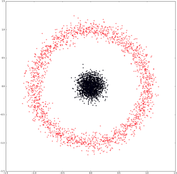
Figure 2-11. Nonspherical data distribution
Hierarchical clustering
Unlike the k-means algorithm, hierarchical clustering methods are not parametrized by an operator-selected value k (the number of clusters you want to create). Choosing an appropriate k is a nontrivial task, and can significantly affect clustering results. Agglomerative (bottom-up) hierarchical clustering builds clusters as follows (illustrated in Figure 2-12):
-
Assign each data point to its own cluster (Figure 2-12, bottom layer).
-
Merge the two clusters that are the most similar, where “most similar” is determined by a distance metric such as the Euclidean distance or Mahalanobis distance.
-
Repeat step 2 until there is only one cluster remaining (Figure 2-12, top layer).
-
Navigate the layers of this tree (dendrogram) and select the layer that gives you the most appropriate clustering result.
Divisive (top-down) hierarchical clustering is another form of hierarchical clustering that works in the opposite direction. Instead of starting with as many clusters as there are data points, we begin with a single cluster consisting of all data points and start dividing clusters based on the distance metric, stopping when each data point is in its own separate cluster.
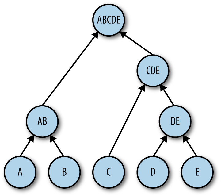
Figure 2-12. Agglomerative hierarchical clustering dendrogram
There are some important points to take note of when considering whether to use hierarchical clustering:
-
Hierarchical clustering produces a dendrogram tree model, as illustrated in Figure 2-12. This model can be more complex to analyze and takes up more storage space than the centroids produced by k-means, but also conveys more information about the underlying structure of the data. If model compactness or ease of analysis is a priority, hierarchical clustering might not be your best option.
-
k-means works with only a small selection of distance metrics (mostly Euclidean distance) and requires numerical data to work. In contrast, hierarchical clustering works with almost any kind of distance metric or similarity function, as long as it produces a result that can be numerically compared (e.g., C is more similar to A than to B). You can use it with categorical data, mixed type data, strings, images, and so on as long as an appropriate distance function is provided.
-
Hierarchical clustering has high time complexity, which makes it unsuitable for large datasets. Taking n to be the number of data points, agglomerative hierarchical clustering has a time complexity of , and naive divisive clustering has a time complexity of .
Locality-sensitive hashing
k-means is good for determining which items are close together when each item can be represented as a sequence of numbers (i.e., a vector in a vector space). However, many items that you would want to cluster do not easily admit such a representation. The classic example is text documents, which are of variable length and admit essentially an infinite choice of words and word orders. Another example is lists, such as the set of IP addresses accessed by a given user, or the set of all of a user’s friends in a social graph.
One very common similarity metric for unordered sets is Jaccard similarity. Jaccard similarity is defined to be the proportion of common items between two sets, out of all the items in the two sets. More precisely, for two sets X and Y, the Jaccard similarity is defined as follows:
To generate clusters when your items are sets, all you need to do is find the groups of items whose Jaccard similarities are very high. The problem here is that this computation is quadratic in the number of items—so as your dataset grows, finding the clusters will quickly become impossible. Locality-sensitive hashing (LSH) attempts to solve this problem. LSH is not normally considered a clustering algorithm, but you can use it as a method for grouping similar items together according to some notion of “distance,” effectively achieving a similar effect to other more typical clustering algorithms.
If the items you want to cluster are not unordered sets (e.g., a text document), the first step is to convert them into sets. For text documents, the most straightforward conversion is into a bag of words—simply, a list of all the words that are included in the document. Depending on your implementation, repeated words might or might not be included multiple times in your list, and/or “stopwords” such as “a,” “the,” and “of” might be excluded.
However, the bag-of-words conversion loses an important aspect of a text document, namely the ordering of the words. To retain information about the ordering, we generalize the conversion into shingling: taking our list to be (overlapping) sequences of consecutive words in the document. For example, if the document was “the quick brown fox jumps over the lazy dog,” the three-word shingles would be:
{(the, quick, brown), (quick, brown, fox), (brown, fox, jumps), (fox, jumps, over), (jumps, over, the), (over, the lazy), (the, lazy, dog)}
You also can perform shingling at the character level, which can be useful for short documents or text strings that can’t be parsed into words.
Now, given a dataset consisting of unordered sets, the question is how to efficiently determine which ones are similar to one another according to the Jaccard metric. The first step is to convert each set into a short “signature,” in such a way that documents that are similar have similar signatures. The standard algorithm for this task is MinHash, which works as follows:
-
Choose k independent hash functions hi that take arbitrary data and output 32-bit integers.
-
Given an item x = {x1, …, xn}, for each i, let mi(x) = min({hi(x1), … hi(xn)}).
-
Output the signature H(x) = (m1(x), …, mk(x)).
The key property of this algorithm is that if the hash functions you choose behave sufficiently randomly, then for two items x and y, the probability that is equal to the Jaccard similarity of x and y.33 Because we use k independent hash functions, we can estimate simply by counting the number of collisions and dividing by k; the estimate becomes more accurate as k increases.
Now that we have computed the MinHash signatures, the key property that we just looked at implies that two elements with highly overlapping signatures have high Jaccard similarities. Thus, to produce clusters of similar items, we must find groups of signatures that overlap in many places. There are two established ways to do this:
-
For each i, compute the reverse mapping from to all the elements x that have that particular hash value. Now for a given element , we can look up all the x that match , and keep the ones that match in at least t places.
-
Reorganize the k hashes into b buckets, each consisting of r “rows.” Let L be a second hash function that maps the hashes in a row to a fixed-size string. We can group together elements whose hashes L match on all rows in at least one bucket. Tuning the values of b and r allows us to trade off false positives (i.e., dissimilar items where L matches) and false negatives (i.e., similar items where L doesn’t match): a higher b reduces false negatives, whereas a higher r reduces false positives. For further details, see Chapter 3 of Mining of Massive Datasets, 2nd ed., by Jure Leskovek, Anand Rajaraman, and Jeffrey D. Ullman (Cambridge University Press).
MinHash is just one example of a locality-sensitive function; that is, one that maps elements that are close together in the input space to values that are close together in the output space. If you measure “closeness” by some metric other than Jaccard similarity—for example, Euclidean distance or Hamming distance—there are specific functions that you can use instead of MinHash in the above procedure; Lescovec et al. provide further details.
k-d trees
A k-dimensional (k-d) tree is a binary tree that stores data in a format optimized for multidimensional spatial analysis. k-d tree construction can be viewed as the pre-processing step of k-NN classification algorithms, but it can also be thought of as its own clustering algorithm. As in hierarchical clustering, the algorithm creates a tree structure, but here the clusters are stored in the leaves rather than in interior nodes.
The typical algorithm used to construct k-d trees proceeds as follows. For each non-leaf node, do the following:
-
Choose a dimension to split on.
-
Choose a split point (e.g., the median of this dimension in the node’s feature subspace).
-
Split the subspace according to the chosen dimension and split point.
-
Stop splitting subspaces when the subspace contains fewer than the number of samples per subspace, leaf_size (e.g., if leaf_size == 1, every leaf node in the tree should represent a feature subspace that contains only one sample).
This procedure results in a binary search tree of feature subspaces, where the combination of all leaf node subspaces makes up the entire feature space. When building k-d tree models for nearest neighbor searches, the space-partitioning binary tree needs to be stored in addition to the training data points. Furthermore, additional data about which samples belong to which leaf nodes needs to be stored in the model, which makes the model even more space inefficient than vanilla k-NN models.
You can use k-d trees to speed up nearest neighbor searches (e.g., during k-NN classification). When searching for the k nearest neighbors of a sample x:
-
Starting from the root of the tree, traverse the tree looking for the node representing the feature subspace that contains x.
-
Analyze the feature subspace containing x:
-
If leaf_size == k, return all points in this subspace as the result.
-
If leaf_size > k, do an exhaustive (brute-force) search within this feature subspace for the k points closest to x, and return those k points as the result.
-
If leaf_size < k, save all points in the subspace as part of the result and continue to the next step.
-
-
Traverse one step up the tree and analyze the feature subspace represented by that node, continuing to add neighbor points to the result until all k neighbors have been found. Repeat this step as necessary to obtain k points.
Similar to the k-NN algorithm, k-d trees are usually not suitable for high-dimensional data,34 and they are even bulkier than k-NN models. Nevertheless, they are very useful for quickly finding nearest neighbors, with an average-case time complexity of . Variations of k-d trees have been developed to address various issues with this algorithm; one example is quadtrees, which are optimized for searching in two-dimensional spaces.
DBSCAN
Density-Based Spatial Clustering of Applications with Noise35 (DBSCAN) is one of the most popular and widely used clustering algorithms because of its generally good performance in different scenarios. Unlike with k-means, the number of clusters is not operator-defined but instead inferred from the data. Unlike hierarchical clustering, which is distance-based, DBSCAN is a density-based algorithm that divides datasets up into subgroups of high-density regions. Let’s consider some of the terminology introduced by this algorithm:
-
The operator passes two parameters into the algorithm:
-
ε defines the radius around a certain point within which to search for neighbors.
-
minPoints is the minimum number of points required to form a cluster.
-
-
Each data point is classified as a core point, a border point, or a noise point:
-
Core points are points that have at least minPoints number of points within their ε-radius.
-
Border points are themselves not core points, but are covered within the ε-radius of some core point.
-
Noise points are neither core points nor border points.
-
In naive implementations, this classification step is done by iterating through each point in the dataset, calculating its distance to all other points in the dataset, and then associating each point with its neighbors (points that are closer than ε distance away from it). With this information, you can tag all points as either core, border, or noise points. After classifying all the data points in the dataset as one of these three types of points, the DBSCAN algorithm proceeds as follows:
-
Select a point P at random out of all unvisited points.
-
If P is not a core point, mark it as visited and continue.
-
If P is a core point, form a cluster around it, and recursively find and usurp all other points within the ε-radius of P as well as any other point that is in the ε-radius of all core points usurped by this cluster.
Let’s say there exists a core point Q within the ε-radius of P. Q (along with all its border points) will be added to the cluster formed around P. If there is another core point R within the ε-radius of Q, core point R (along with all its border points) will also be added to the cluster formed around P.
This recursive step is repeated until there are no more core points to usurp.
-
Repeat until all points in the dataset have been visited.
Even though DBSCAN has been shown to work very well in a variety of situations, there are some caveats:
-
DBSCAN does not work well when clusters in the dataset have different densities. This makes it difficult to select values of ε and minPoints that are suitable for all clusters in the data. Ordering Points to Identify the Clustering Structure (OPTICS)36 is an algorithm very similar to DBSCAN that addresses this weakness by introducing spatial ordering into the point selection process, albeit at the cost of speed.
-
Careful selection of parameters ε and minPoints is important for good performance of the algorithm. It can be challenging to select good values for these unless you have a good understanding of the data’s distribution and densities.
-
The algorithm is nondeterministic and can produce different results depending on which points are first visited in the random selection in step 1.
-
DBSCAN performs poorly on high-dimensional data because it most commonly uses the Euclidean distance as a distance metric, which suffers from the “curse of dimensionality.”
-
If your dataset is produced by sampling a raw source, the sampling method that you use can significantly alter the density characteristics of the data. Density-based algorithms will then be unsuitable because the results they produce rely on an accurate representation of the data’s true density characteristics.
Evaluating Clustering Results
It can sometimes be difficult to make sense of the results of clustering operations. Evaluating supervised learning algorithms is a much more straightforward task because we have access to the ground truth labels: we can simply count the number of samples to which the algorithm correctly and wrongly assigns labels. In the case of unsupervised learning, it is unlikely we have access to labels, though if we do evaluation becomes much easier.37,38 For example, commonly used metrics for evaluating clustering results if the ground truth labels are known are:
- Homogeneity
-
The degree to which each cluster contains only members of a single class.
- Completeness
-
The degree to which all members of a certain class are assigned to the same cluster.
The harmonic mean of these two metrics is known as the V-measure,39 an entropy-based score representing the clustering operation’s accuracy, which has the formula:
where h is homogeneity and c is completeness.
We will use the scikit-learn implementations of these clustering evaluation metrics in Chapter 5.
On the other hand, the fact that we are considering clustering at all means it is likely that we do not have any ground truth labels for our dataset. Instead, we can no longer use the V-measure because both homogeneity and completeness can be measured only by comparing prediction labels to ground truth labels. In this case, we have to rely on signals derived directly from the trained model itself. Essentially, we consider the clustering operation to be successful if samples assigned to the same cluster are all similar to one another, and samples assigned to different clusters are all completely dissimilar from one another. There are two popular ways to measure this:
- Silhouette coefficient
-
This score is calculated separately for each sample in the dataset. Using some distance metric (e.g., Euclidean distance), we find the following two mean distances for some sample x:
-
a: the mean distance between sample x and all other samples in the same cluster
-
b: the mean distance between sample x and all other samples in the next nearest cluster
The Silhouette coefficient s is then defined as follows:40
For a clustering result that is hugely incorrect, the a will be much larger than b, resulting in the numerator being negative. Because the denominator will never be negative (distance metrics do not take on negative values), s will itself be negative. In fact, s is bounded between −1 and +1. The closer s is to +1, the better the clustering result. When s is very close to 0, we have highly overlapping clusters. Nevertheless, it is found that the Silhouette coefficient is biased toward distance-based (e.g., k-means), grid-based (e.g., STING41), and hierarchical clustering algorithms that produce convex clusters. It does not work well for clusters produced by density-based algorithms such as DBSCAN and OPTICS, because neither a nor b take cluster density into consideration. Also, because the Silhouette coefficient must be independently calculated for each sample in the dataset, it can be quite slow.
-
- Calinski-Harabaz index
-
The Calinski-Harabaz (C-H) index42 is higher (better) when clusters are dense and well separated. By most measures, this measure of clustering effectiveness is closer to how humans evaluate clustering results. We consider a clustering result to be good if there are visibly separated and densely gathered groups of samples. The C-H index uses two measures:
-
: the within-cluster dispersion, a matrix of distances between samples in a cluster and the geometric center of the cluster
-
: the between-group dispersion, a matrix of distances between the center of a cluster and the centers of all other clusters
(Here, k is the number of clusters in the model.)
The C-H score (s) takes the ratio of and (where N is the number of samples in the dataset and tr is the trace of the matrix43):
The C-H score can be computed much more efficiently than the Silhouette index. Even though it is still biased against density-based clusters, it is comparatively more reliable than the Silhouette index.
-
No matter which method you choose, there will be some inherent limitations in evaluating clustering results without any human labeling. If you suspect that clustering models are not performing well in practice in spite of good evaluation metrics, it may be necessary to invest resources in manually labeling a subset of samples and use semi-supervised approaches to evaluate the model.
Conclusion
Machine learning, at its most basic, is the process of using historical data to derive a prediction algorithm for previously unseen data. In this chapter, we focused on classification (i.e., determining which category each data point belongs to) and clustering (i.e., determining which data points are similar to each other). Classification can be supervised, in which case the historical data comes with class labels; the unsupervised case, in which there are no (or very few) historical labels, is more amenable to clustering.
We described, at a high level, a number of commonly used classification and clustering algorithms, and we made some sense of which tasks each algorithm is good at. The details behind all of these algorithms could fill an entire textbook; indeed, Hastie, Tibshirani, and Friedman cover much of the applicable theory in their book The Elements of Statistical Learning (Springer), and we recommend it if you are interested.
The algorithms we discussed require a significant amount of data to be effective—the more data, the better. But what happens if the event you are trying to detect is very rare? Solving this problem will be the subject of the next chapter.
1 Simple algorithms like this one are usually called “rules.”
2 You can find the dataset in chapter2/datasets/payment_fraud.csv in our code repository.
3 For more information on Pandas DataFrames, see the documentation.
4 This is not true for all machine learning algorithms. For example, decision trees do not require any or all features to be numeric. The advantage of expressing features in numeric terms is that each data point can be expressed as a vector in a real vector space, and we can apply all the techniques of linear algebra and multivariable calculus to the problem.
5 Typically, we’ll set the pd.get_dummies() argument drop_first to True to avoid the so-called “dummy variable trap,” in which independent variables being closely correlated violates assumptions of independence in regression. We chose to keep things simple to avoid confusion, but elaborate on this problem in Chapter 5.
6 You can find this example as a Python Jupyter notebook in our repo at chapter2/logistic-regression-fraud-detection.ipynb.
7 Technically, a differentiable, oriented surface.
8 The full background for why this particular function is selected as the hypothesis function for binary logistic regression is slightly more involved, and we will not go into much more detail here. For further details, see section 4.4 of The Elements of Statistical Learning, 2nd ed., by Trevor Hastie, Robert Tibshirani, and Jerome H. Friedman (Springer).
9 A seminal book that defined the field of convex optimization (note that not all optimization problems we speak of may be convex in nature) is Convex Optimization by Stephen P. Boyd and Lieven Vandenberghe (Cambridge University Press).
10 Rong-En Fan et al., “LIBLINEAR: A Library for Large Linear Classification,” Journal of Machine Learning Research 9 (2008): 1871–1874.
11 Francis Bach, “Stochastic Optimization: Beyond Stochastic Gradients and Convexity.” INRIA - Ecole Normale Supérieure, Paris, France. Joint tutorial with Suvrit Sra, MIT - NIPS - 2016.
12 Stephen Boyd et al., “Distributed Optimization and Statistical Learning via the Alternating Direction Method of Multipliers,” Foundations and Trends in Machine Learning 3 (2011): 1–122.
13 For an event X that occurs with probability p, the odds of X are , and the log odds are .
14 This assumption is not exclusive to logistic regression. Most other machine learning algorithms also require that features be uncorrelated.
15 For performing logistic regression on smaller datasets, consider using exact logistic regression.
16 Note that as of late 2017, scikit-learn’s implementation of decision trees (sklearn.tree.DecisionTreeClassifier and other tree-based learners) does not properly handle categorical data. Categorical variables encoded with integer labels (i.e., with sklearn.preprocessing.LabelEncoder and not sklearn.preprocessing.OneHotEncoder or the pandas.get_dummies() function) will be incorrectly treated as numerical variables. Even though a scikit-learn maintainer claimed that models like sklearn.tree.RandomForestClassifier tend to be “very robust to categorical features abusively encoded as integer features in practice,”, it is still highly recommended that you convert categorical variables to dummy/one-hot variables before feeding them into sklearn decision trees. There should be a new feature for tree-based learners to have support for categorical splits (up to 64 categories per feature) in 2018.
17 Laurent Hyafil and R.L. Rivest, “Constructing Optimal Binary Decision Trees is NP-Complete,” Information Processing Letters 5:1 (1976): 15–17.
18 For classification problems with p total features, is recommended. For regression tasks, is recommended. Refer to section 15.2 of The Elements of Statistical Learning, 2nd ed., by Trevor Hastie, Robert Tibshirani, and Jerome Friedman.
19 There also exist variants of random forests that limit the set of features available to an individual decision tree; for example, if the total feature set is {A,B,C,D,E,F,G}, all split points made in decision tree 1 might randomly select only three features out of the subset of features {A,B,D,F,G}.
20 Tianqi Chen and Carlos Guestrin, “XGBoost: A Scalable Tree Boosting System,” Proceedings of the 22nd ACM SIGKDD International Conference on Knowledge Discovery and Data Mining (2016): 785–794.
21 See section 5.8 and Chapter 12 of The Elements of Statistical Learning by Trevor Hastie, Robert Tibshirani, and Jerome Friedman.
22 David Freeman, “Using Naive Bayes to Detect Spammy Names in Social Networks,” Proceedings of the 2013 ACM Workshop on Artificial Intelligence in Security (2013): 3–12.
23 k-NN can also be used for regression—typically, the average of a test sample’s k nearest neighboring sample labels is taken to be the prediction result.
24 Jon Louis Bentley, “Multidimensional Binary Search Trees Used for Associative Searching,” Communications of the ACM 18 (1975): 509–517.
25 We explain the concept of class imbalance in greater detail in Chapter 5.
26 W.S. McCulloch and W.H. Pitts, “A Logical Calculus of Ideas Immanent in Nervous Activity,” Bulletin of Mathematical Biophysics 5 (1942): 115–133.
27 This oversimplification of how ANNs work barely does justice to the field. For a more complete discussion of this topic, read Deep Learning by Ian Goodfellow, Yoshua Bengio, and Aaron Courville (MIT Press).
28 Most tree-based estimators like DecisionTreeClassifier and RandomForestClassifier, as well as some ensemble estimators like GradientBoostingClassifier, have the feature_importances_ attribute. Generalized linear models such as LinearRegression and LogisticRegression and support vector machines such as SVC have the coef_ attribute, allowing SelectFromModel to compare magnitudes of the coefficients or importances corresponding to each feature.
29 Using the mean as a feature importance threshold is the default strategy of SelectFromModel unless you specify the threshold parameter as something else; for example, median or a static value.
30 You can find an example of applying sklearn.feature_selection.SelectFromModel to a real problem in a Python Jupyter notebook in chapter2/select-from-model-nslkdd.ipynb from our code repository.
31 The default method that most machine learning libraries use to deal with this is to pick the class that has the highest score and use that as the prediction result. For instance, for a binary classification problem this simply translates to a threshold of 50%, but for a three-class (or more) classification problem the class with the highest probability/confidence is selected as the classifier’s prediction result.
32 If the AUC is less than 0.5, by reversing the classifier labels you can produce a classifier with AUC > 0.5.
33 Let’s try to understand why this property holds. To begin, we can simplify by assuming that there are no collisions between hash functions, so the are all distinct, and therefore implies that there are some such that ; or in other words, the minimal hash is of an element common to the two sets. Now consider all the elements of as a set . If the hash function looks random, the probability that the smallest is in the intersection is exactly , which is .
34 For high-dimensional feature spaces, k-d trees will perform similarly to a brute-force linear search.
35 Ram Anant, et al., “A Density Based Algorithm for Discovering Density Varied Clusters in Large Spatial Databases,” International Journal of Computer Applications 3:6 (2010).
36 Mihael Ankerst, et al., “OPTICS: Ordering Points to Identify the Clustering Structure,” SIGMOD Record 28:2 (1999): 49–60.
37 W.M. Rand, “Objective Criteria for the Evaluation of Clustering Methods,” Journal of the American Statistical Association 66 (1971): 846–850.
38 Nguyen Xuan Vinh, Julien Epps, and James Bailey, “Information Theoretic Measures for Clustering Comparison: Is a Correction for Chance Necessary?”, Proceedings of the 26th Annual International Conference on Machine Learning (2009): 1073–1080.
39 Andrew Rosenberg and Julia Hirschberg, “V-Measure: A Conditional Entropy-Based External Cluster Evaluation Measure,” Proceedings of the 2007 Joint Conference on Empirical Methods in Natural Language Processing and Computational Natural Language Learning (2007): 410–420.
40 Peter Rousseeuw, “Silhouettes: A Graphical Aid to the Interpretation and Validation of Cluster Analysis,” Journal of Computational and Applied Mathematics 20 (1987): 53–65.
41 Wei Wang, Jiong Yang, and Richard Muntz, “STING: A Statistical Information Grid Approach to Spatial Data Mining,” Proceedings of the 23rd International Conference on Very Large Data Bases (1997): 186–195.
42 Tadeusz Caliński and J.A. Harabasz, “A Dendrite Method for Cluster Analysis: Communications in Statistics,” Theory and Methods 3 (1974): 1–27.
43 The trace of a matrix is defined to be the sum of the elements on the diagonal (upper left to lower right).