Neural Networks

What we expect from a computer is that we provide some inputs and then receive outputs that match our needs. Scientists try to mimic the human brain by creating an intelligence machine—a machine that does the same reasoning as humans.

The most important element of the human brain is neurons. Human brains consist of 75 million neurons. Each neuron is connected to others via synapses. So what we have in a neural network are some nodes that are connected to one another. In the human body, if a neuron is triggered by some external element, it will pass the message from the receiver node to other nodes, via synapsis. (Figure 7-1).

Neural networks mimic the same concepts as the human brain. One node gets some input from the environment, and the neural network model creates outputs that produce the result just as a computer system would (Figure 7-2).

Some of the connections are more important than others, meaning that they have a greater impact on the results than others. In neural networks, we refer to this importance as the connections’ weights.

Another analogy that better expresses the goal of a neural network is the descent after climbing a mountain. When we reach the summit and the weather is foggy, we are only able to see one meter ahead. We must decide which direction to choose with only one meter of visibility. We take a first step based on the location, again deciding which direction to follow and taking other steps. So, with each step we are evaluating the course and choosing the best way to come down from the mountain (Figure 7-3).

Each decision can be viewed as a node that leads us to a better and faster resolution. In a neural network, there are some hidden nodes that perform the main task. They find the best value for the output while using a function called an activation function.

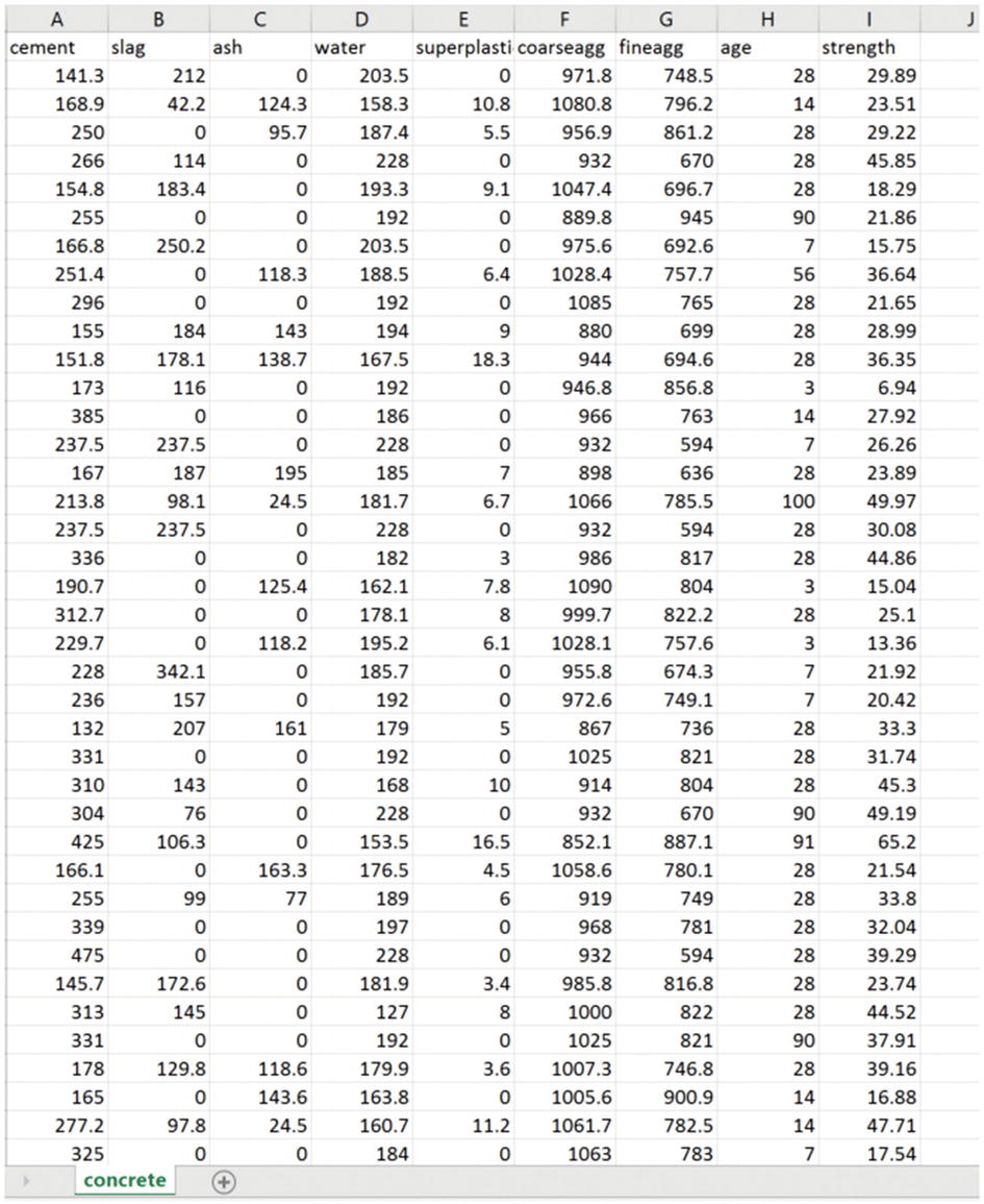
In this section, I am going to refer to an example from Machine Learning with R [1]. The example is about predicting the strength of concrete. The concrete has been used in many different structures, such as a bridge, apartment, roadways, and so on. For safety, the strength of the concrete is critical. The concrete’s strength depends on the material used to create it, such as cement, slag, ash, water, and so forth. We have a data set of the ingredients of the concrete (Figure 7-4). You can download it from “Machine Learning with R datasets” [2].

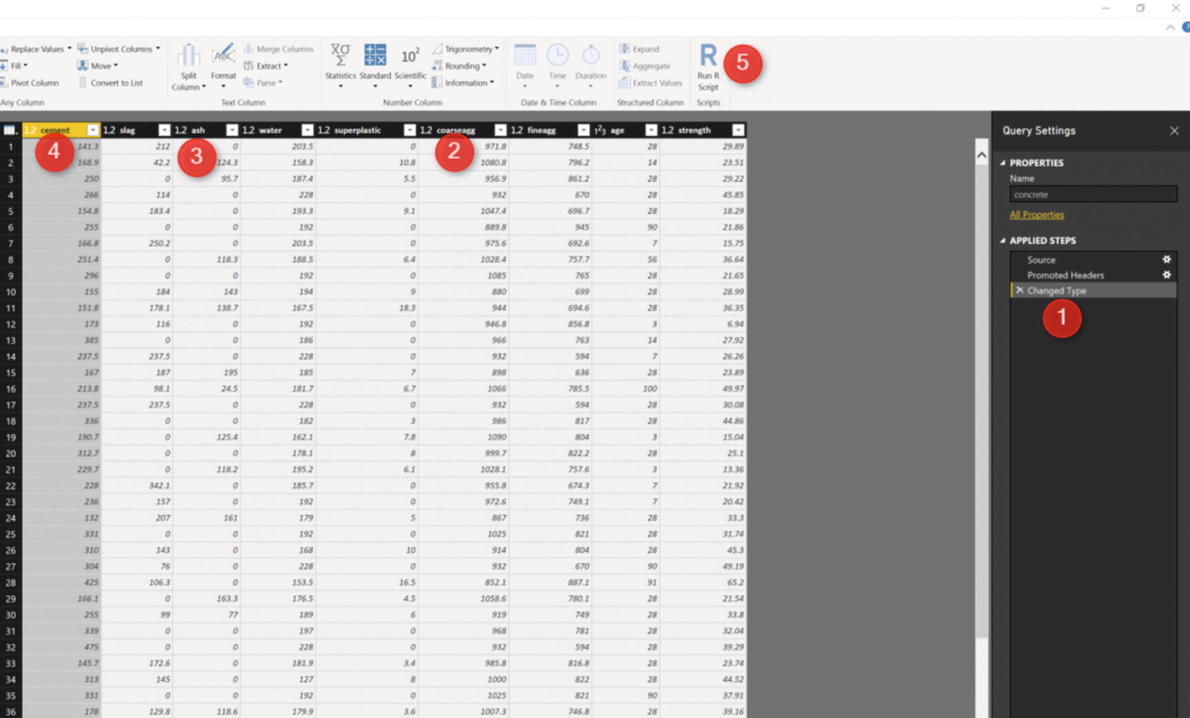
A neural network can be used for predicting a value or class, or it can be used for predicting multiple things. In our example, we are going to predict a value, that is, the strength of concrete. First, we load the data in Power BI, and in Query Editor, we write some R codes. Then we must make some data transformations (Figure 7-5).

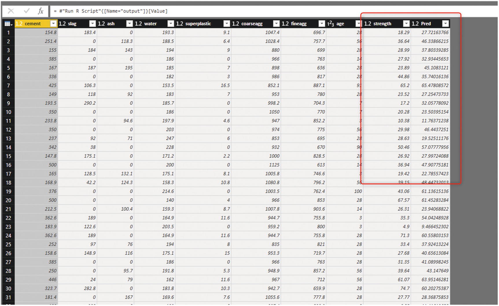
The result will be stored in an output variable that is in a data frame structure. Another important consideration is that Power Query only recognizes the data. Frame format. So, other data structures, such as vectors, lists, and matrices cannot be shown in the Power Query editor (Figure 7-6).

It is possible to see the neural network structure in the visualization area, to see the hidden node, layer, and so forth. Therefore, we must duplicate the data set for concrete in Power BI Report, using the R custom visual, as shown in Figure 7-7. Next, we must write the same codes for neural network prediction and add another line for plotting the model. Run the code, and you will see the neural network structure that has just appeared on the layer, and the error is 3.001.

normalize <- function(x) {

    return((x - min(x)) / (max(x) - min(x)))

}

concrete_norm <- as.data.frame(lapply(dataset, normalize))

summary(concrete_norm$strength)

concrete_train <- concrete_norm[1:773,]

concrete_test <- concrete_norm[774:1030,]

library("neuralnet")

      concrete_model <- neuralnet(strength ~ cement + slag

      + ash + water + superplastic + coarseagg + fineagg + age,

      data = concrete_train)

plot(concrete_model)

We can mitigate the error by changing the number of hidden nodes and layers.

Decision Trees

A decision tree is a common approach for doing machine learning. This tool can be used for prediction, descriptive analysis, and feature selection. A decision tree follows the way that we reach decisions. Imagine a job seeker who wants to decide among a number of different jobs. He or she has established some criteria for his/her selection, such as the following: What are the responsibilities? What is the annual salary or hourly rate? Finally, how many times a year is travel required? We can simulate the job seeker’s decision-making process, as shown in Figure 7-8. The root of the tree is the main decision point, that is, saying yes or no to the job. Then the most important criterion is whether the job title matches the searcher’s expertise. The second most important criterion is salary. Finally, if there is no leaf, the third criterion is to check the number of required travel days per year. The decision tree uses information gain theory to identify what is the main criteria are for tree branching. Details on how this works are available at http://radacad.com/decision-tree-conceps-part-1 [3].

There are different ways of using decision trees in Power BI. One approach involves Power BI custom visualization.

To access this, you first must sign in to a Power BI account (Figure 7-9).

We must retrieve the visual from the Visualization panel by clicking the three dots and then choosing the Import from store option (Figure 7-10).

On the Power BI custom visual page, there are different categories of visuals, including Filters, KPIs, Maps, Advanced Analytics, and more (Figure 7-11).

You need only click the Advanced Analytics option and then select Decision Tree Chart (Figure 7-12). Click the Add button to add the chart to Power BI visualization.

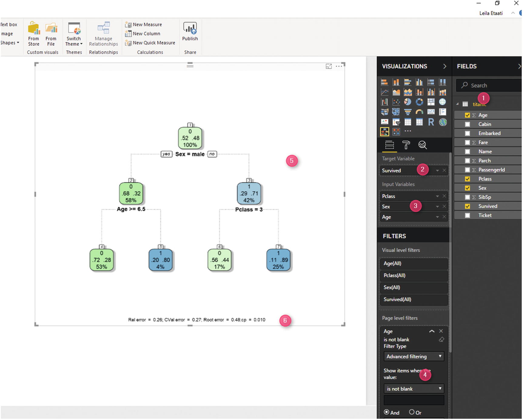
To test the custom visual, we must import some data into Power BI Desktop for predictive analysis. The data is a free data set about the Titanic disaster [4]. We must choose the fields for decision making. The main aim (target) is to predict whether people survived. To do that, first we have to choose a couple of columns that may affect passenger survival, such as age, gender, and passenger class. Next, put the Survived column as the target variable, in the related data field (Figure 7-14).

The next step is to remove the missing values (“blank”) from the age column. Finally, the related decision tree chart appears in Power BI Report (Figure 7-14).

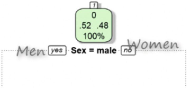
At the root of tree, there are four numbered tags. 0 stands for passengers who could not have survived. Also, these people are identified by a green tag. The “100%” means that all data is at the root. The “0.52” and “0.48” indicate that about 0.52 are men and 0.48 are women. In other words, the first attribute that the decision tree decided to analyze (based on entropy theory) is the gender of the passengers (Figure 7-15).

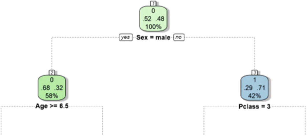
For the next level, on the left, the tag is in green, and it already branches to represent the male passengers. Based on that branch, we can summarize that most of the male passengers did not survive (0). However, as you can see in Figure 7-16, for women (the branch at the right side), the attribute that is going to be analyzed is passenger class.

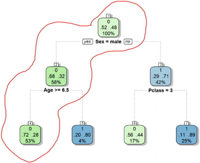
For men (root) older than seven years of age (second node), there is a 58% possibility that they will not survive (green tag and 0) (Figure 7-17).

Men (root) older than seven years old (second node) will not survive (green tag and 0), with the possibility of 53%. Also, males younger than seven will survive.

A decision tree inside Power Query can be used to do machine learning and show the result in Power BI Report (the same process that has been explained in the “Neural Networks” section).

In the next section, I am going to write R code for a decision tree inside Power Query and show how it is possible to pass parameters to it.

Automated Machine Learning Inside Power Query

In the previous section, I explained how decision trees can be used for prediction analysis. Now we are going to use it inside Power Query, for predictions without a specific chart.

First, we must click the Power Query Editor at the top of the page, to navigate to the Power Query environment. In Power Query, you must first download the data set for the Titanic from www.kaggle.com/c/titanic [4]. Then, click New Source, select the Text/CSV option to import the data set, and click OK (Figure 7-18).

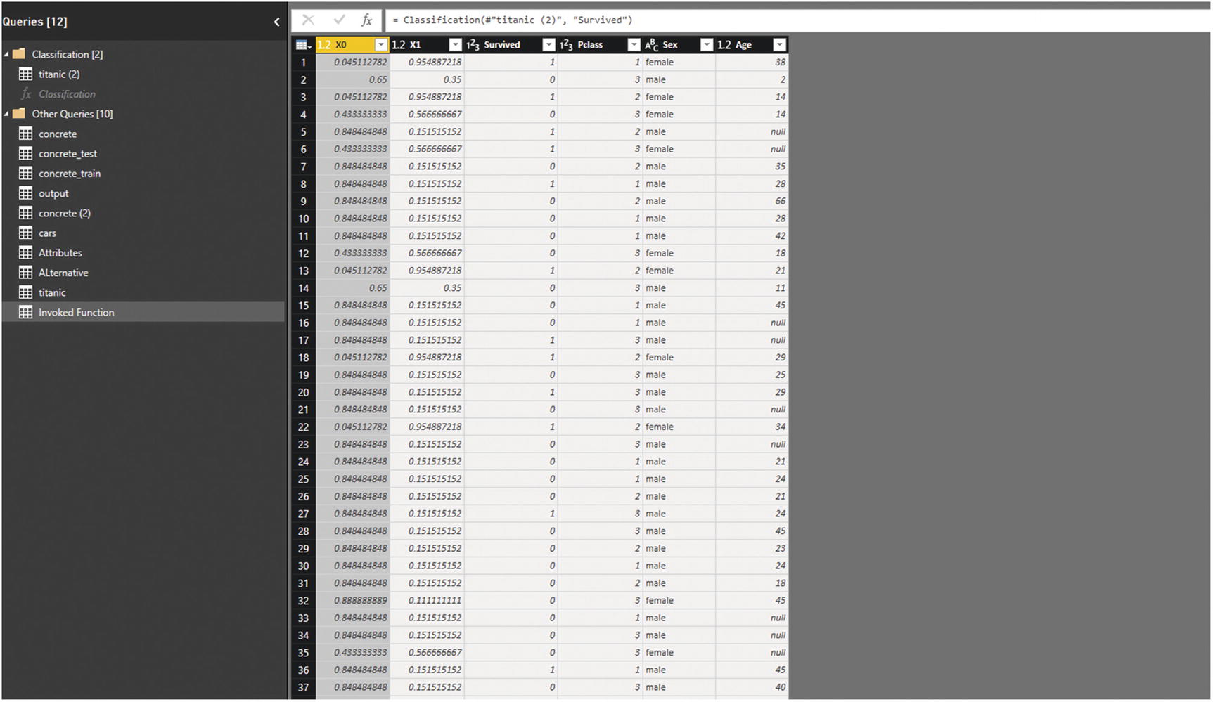
So, the result of the prediction will be shown in Power Query, with the name rpartresult. The result will consist of two different additional columns. “X0” stands for the probability of passengers not surviving, and “x1” is the probability of passengers surviving. Now imagine that we want to use the rpart algorithm for classifying another data set, such as the cancer-related data discussed in Chapter 6. It is possible to parameterize the R code for passing the desired data set, prediction column, and so forth, to the R codes. To do this, we must duplicate the data set (Figure 7-19).

Now just right-click the new data set, to create a function out of it. There is a need to create a function from the new duplicated data set (Figure 7-20).

After creating a function, we must customize it, by passing parameters. To do this, we must navigate to Advanced Editor (Figure 7-21).

In Advanced Editor, it is possible to see the steps previously applied to the Titanic data set in M language. As you can see in Figure 7-22, the source of the data set has been identified from my local machine.

After running the code, we will have a function with an input variable (Figure 7-23).

To test the function, we must create a data set to pass to the function. Import the new Titanic data set, then Ctrl+Click the four main columns: Survived, Pclass, Age, and Sex. Next, right-click and select the Remove Columns option (Figure 7-24).

Finally, there is a data set with four columns now ready to pass to the function. In the function, for the first parameter, we must choose the Titanic data set, and for the second, the Prediction Column named Survived (Figure 7-25).

Next, we may get a message for Edit Permission that is about providing permission to run external scripts on the query (Figure 7-26).

After accepting the permission, we can now see the result, as shown in Figure 7-27.

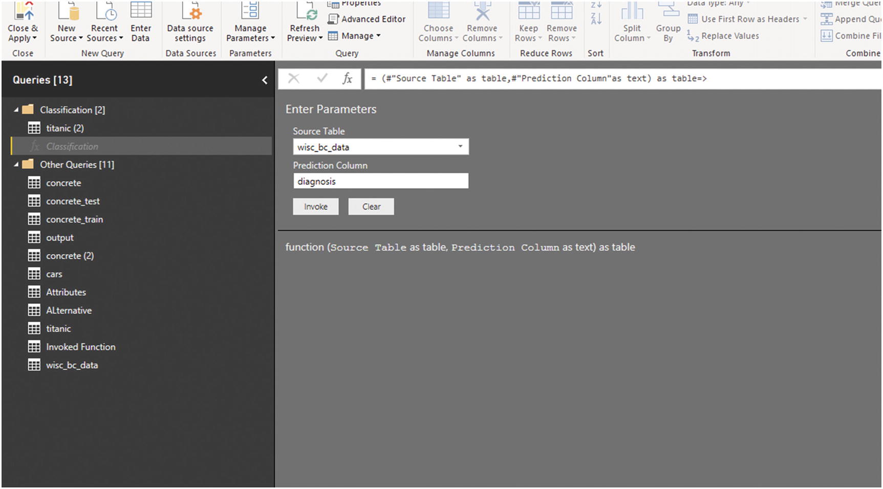
To test the function, I imported another data set [5] that was introduced in Chapter 6. It is a data set related to breast cancer patients. I want to predict patient diagnosis: will a patient’s cancer become malignant “M” or benign “B.” We follow the same process as before for this new data set. First, we import it, then we pass the name and column of the data set to the function (Figure 7-28).

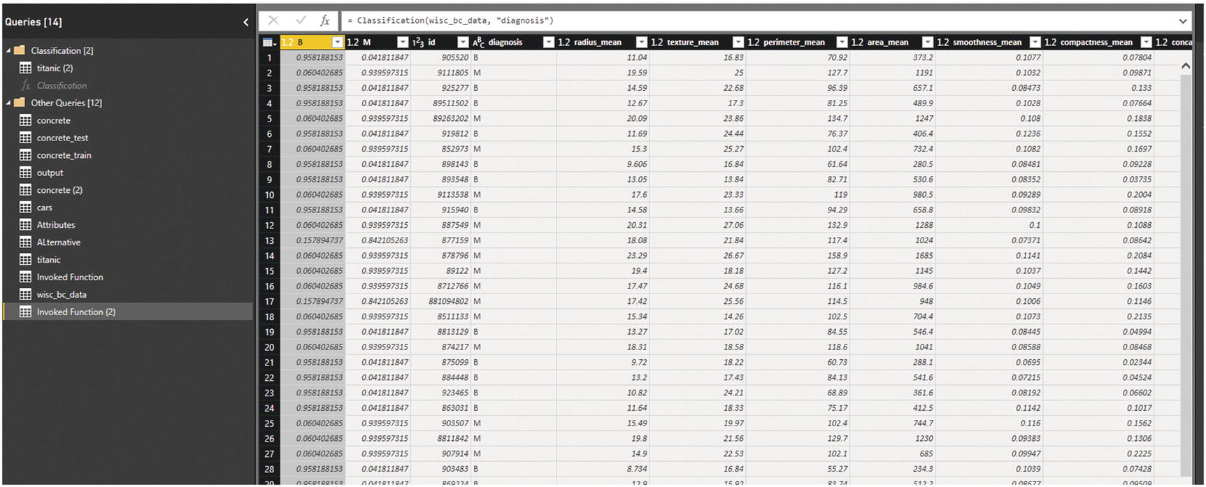
After invoking the function, the prediction result appears as a new query (Figure 7-29).

Summary

The main aim of this chapter was to show how we can perform machine learning inside the Power Query Editor using R codes. Two different algorithms were introduced: neural networks and decision trees. I discussed how you can set parameters for making machine learning much more flexible. In the next chapter, I will discuss descriptive analysis using Power BI.

References