Chapter 9: Introducing Data Frame Analytics
In the first section of this book, we took an in-depth tour of anomaly detection, the first machine learning capability to be directly integrated into the Elastic Stack. In this chapter and the following one, we will take a dive into the new machine learning features integrated into the stack. These include outlier detection, a novel unsupervised learning technique for detecting unusual data points in non-timeseries indices, as well as two supervised learning features, classification and regression.
Supervised learning algorithms use labeled datasets – for example, a dataset describing various aspects of tissue samples along with whether or not the tissue is malignant – to learn a model. This model can then be used to make predictions on previously unseen data points (or tissue samples, to continue our example). When the target of prediction is a discrete variable or a category such as a malignant or non-malignant tissue sample, the supervised learning technique is called classification. When the target is a continuous numeric variable, such as the sale price of an apartment or the hourly price of electricity, the supervised learning technique is known as regression. Collectively, these three new machine learning features are known as Data Frame Analytics. We will discuss each of these in more depth in the following chapters.
Although each of these solves a different problem and has a different purpose, they are all powered under the hood by a common data transformation technology, that of transforms, which enables us to transform and aggregate data from a transaction- or stream-based format into an entity-based format. This entity-centric format is required by many of the algorithms we use in Data Frame Analytics and thus, before we dive deeper into each of the new machine learning features, we are going to dedicate this chapter to understanding in depth how to use transforms to transform our data into a format that is more amenable for downstream machine learning technologies. While on this journey, we are also going to take a brief tour of Painless, the scripting language embedded into Elasticsearch, which is a good tool for any data scientists or engineers working with machine learning in the Elastic Stack.
A rich ecosystem of libraries, both for data manipulation and machine learning, exists outside of the Elastic Stack as well. One of the main drivers powering these applications is Python. Because of its ubiquity in the data science and data engineering communities, we are going to focus, in the second part of this chapter, on using Python with the Elastic Stack, with a particular focus on the new data-science native Elasticsearch client, Eland. We'll check out the following topics in this chapter:
- Learning to use transforms
- Using Painless for advanced transform configurations
- Working with Python and Elasticsearch
Technical requirements
The material in this chapter requires Elasticsearch version 7.9 or above and Python 3.7 or above. Code samples and snippets required for this chapter will be added under the folder Chapter 9 - Introduction to Data Frame Analytics in the book's GitHub repository (https://github.com/PacktPublishing/Machine-Learning-with-Elastic-Stack-Second-Edition/tree/main/Chapter%209%20-%20Introduction%20to%20Data%20Frame%20Analytics). In such cases where some examples require a specific newer release of Elasticsearch, this will be mentioned before the example is presented.
Learning how to use transforms
In this section, we are going to dive right into the world of transforming stream or event-based data, such as logs, into an entity-centric index.
Why are transforms useful?
Think about the most common data types that are ingested into Elasticsearch. These will often be documents recording some kind of time-based or sequential event, for example, logs from a web server, customer purchases from a web store, comments published on a social media platform, and so forth.
While this kind of data is useful for understanding the behavior of our systems over time and is perfect for use with technologies such as anomaly detection, it is harder to make stream- or event-based datasets work with Data Frame Analytics features without first aggregating or transforming them in some way. For example, consider an e-commerce store that records purchases made by customers. Over a year, there may be tens or hundreds of transactions for each customer. If the e-commerce store then wants to find a way to use outlier detection to detect unusual customers, they will have to transform all of the transaction data points for each customer and summarize certain key metrics such as the average amount of money spent per purchase or number of purchases per calendar month. In Figure 9.1, we have a simplified illustration that depicts the process of taking transaction records from e-commerce purchases made by two customers and converting them into an entity-centric index that describes the total quantity of items purchased by these customers, as well as the average price paid per order.
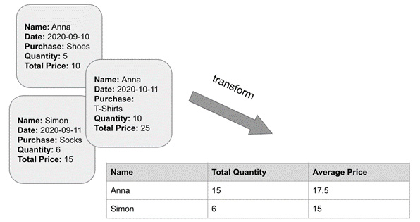
Figure 9.1 – A diagram illustrating the process of taking e-commerce transactions and transforming them into an entity-centric index
In order to perform the transformation depicted in Figure 9.1, we have to group each of the documents in the transaction index by the name of the customer and then perform two computations: sum up the quantity of items in each transaction document to get a total sum and also compute the average price of purchases for each customer. Doing this manually for all of the transactions for each of the thousands of potential customers would be extremely arduous, which is where transforms come in.
The anatomy of a transform
Although we are going to start off our journey into transforms with simple examples, many real-life use cases can very quickly get complicated. It is useful to keep in mind two things that will help you keep your bearing as you apply transforms to your own data projects: the pivot and the aggregations.
Let's examine how these two entities complement each other to help us transform a stream-based document into an entity-centric index. In our customer analytics use case, we have many different features describing each customer: the name of the customer, the total price they paid for each of their products at checkout, the list of items they purchased, the date of the purchase, the location of the customer, and so forth.
The first thing we want to pick is the entity for which we are going to construct our entity-centric index. Let's start with a very simple example and say that our goal is to find out how much each customer spent on average per purchase during our time period and how much they spent in total. Thus, the entity we want to construct the index for – our pivot – is the name of the customer.
Most of the customers in our source index have more than one transaction associated with them. Therefore, if we try to group our index by customer name, for each customer we will have multiple documents. In order to pivot successfully using this entity, we need to decide which aggregate quantities (for example, the average price per order paid by the customer) we want to bring into our entity-centric index. This will, in turn, determine which aggregations we will define in our transform configuration. Let's take a look at how this works out with a practical example.
Using transforms to analyze e-commerce orders
In this section, we will use the Kibana E-Commerce sample dataset to illustrate some of the basic transformation concepts outlined in the preceding section:
- Import the Sample eCommerce orders dataset from the Kibana Sample data panel displayed in Figure 9.2 by clicking the Add data button. This will create a new index called kibana_sample_data_ecommerce and populate it with the dataset.
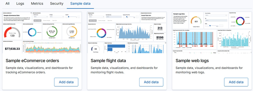
Figure 9.2 – Import the Sample eCommerce orders dataset from the Kibana Sample data panel
- Navigate to the Transforms wizard by bringing up the Kibana slide-out panel menu from the hamburger button in the top left-hand corner, navigating to Stack Management, and then clicking Transforms under the Data menu.
- In the Transforms view, click Create your first transform to bring up the Transforms wizard. This will prompt you to choose a source index – this is the index that the transform will use to create your pivot and aggregations. In our case, we are interested in the kibana_sample_data_ecommerce index, which you should select in the panel shown in Figure 9.3. The source indices displayed in your Kibana may look a bit different depending on the indices currently available in your Elasticsearch cluster.
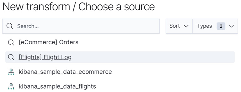
Figure 9.3 – For this tutorial, please select kibana_sample_data_ecommerce
- After selecting our source index, the Transform wizard will open a dialog that shows us a preview of our source data (Figure 9.4), as well as allowing us to select our pivot entity using the drop-down selector under Group by. In this case, we want to pivot on the field named customer_full_name.
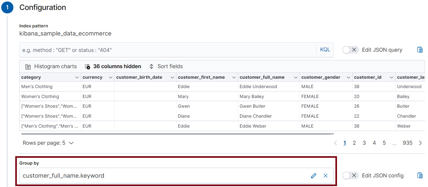
Figure 9.4 – Select the entity you want to pivot your source index by in the Group by menu
- Now that we have defined the entity to pivot our index by, we will move on to the next part in the construction of a transform: the aggregations. In this case, we are interested in figuring out the average amount of money the customer spent in the e-commerce store per order. During each transaction, which is recorded in a document in the source index, the total amount paid by the customer is stored in the field taxful_total_price.
Therefore, the aggregation that we define will operate on this field. In the Aggregations menu, select taxful_total_price.avg. Once you have clicked on this selection, the field will appear in the box under Aggregations and you will see a preview of the pivoted index as shown in Figure 9.5.
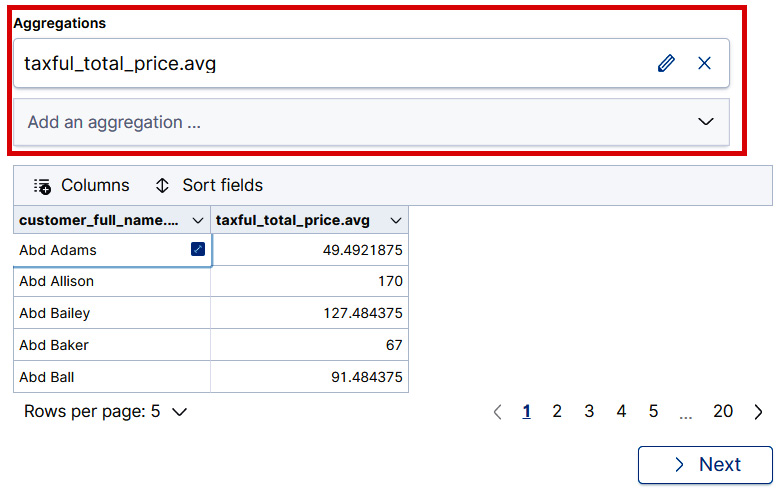
Figure 9.5 – A preview of the transformed data is displayed to allow a quick check that everything is configured as desired.
- Finally, we will configure the last two items: an ID for the transform job, and the name of the destination index that will contain the documents that describe our pivoted entities. It is a good idea to leave the Create index pattern checkbox checked as shown in Figure 9.6 so that you can easily navigate to the destination index in the Discover tab to view the results.
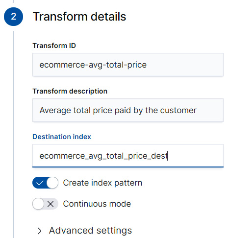
Figure 9.6 – Each transform needs a transform ID
The transform ID will be used to identify the transform job and a destination index that will contain the documents of the entity-centric index that is produced as a result of the transform job.
- To start the transform job, remember to click Next in the Transform wizard after completing the instructions described in step 6, followed by Create and start. This will launch the transform job and create the pivoted, entity-centric index.
- After the transform has completed (you will see the progress bar reach 100% if all goes well), you can click on the Discover button at the bottom of the Transform wizard and view your transformed documents.
As we discussed at the beginning of this section, we see from a sample document in Figure 9.7 that the transform job has taken a transaction-centric index, which recorded each purchase made by a customer in our e-commerce store and transformed it into an entity-centric index that describes a specific analytical transformation (the calculation of the average price paid by the customer) grouped by the customer's full name.

Figure 9.7 – The result of the transform job is a destination index where each document describes the aggregation per each pivoted entity. In this case, the average taxful_total_price paid by each customer
Congratulations – you have now created and started your first transform job! Although it was fairly simple in nature, this basic job configuration is a good building block to use for more complicated transformations, which we will take a look at in the following sections.
Exploring more advanced pivot and aggregation configurations
In the previous section, we explored the two parts of a transform: the pivot and the aggregations. In the subsequent example, our goal was to use transforms on the Kibana sample eCommerce dataset to find out the average amount of money our customers spent per order. To solve this problem, we figured out that each document that recorded a transaction had a field called customer.full_name and we used this field to pivot our source index. Our aggregation was an average of the field that recorded the total amount of money spent by the customer on the order.
However, not all questions that we might want to ask of our e-commerce data lend themselves to simple pivot or group by configurations like the one discussed previously. Let's explore some more advanced pivot configurations that are possible with transforms, with the help of some sample investigations we might want to carry out on the e-commerce dataset. If you want to discover all of the available pivot configurations, take a look at the API documentation for the pivot object at this URL: https://www.elastic.co/guide/en/elasticsearch/reference/master/put-transform.html.
Suppose that we would like to find out the average amount of money spent per order per week in our dataset, and how many unique customers made purchases. In order to answer these questions, we will need to construct a new transform configuration:
- Instead of pivoting by the name of the customer, we want to construct a date histogram from the field order_date, which, as the name suggests, records when the order was placed. The Transform wizard makes this simple since date_histogram(order_date) will be one of the pre-configured options displayed in the Group by dropdown.
- Once you have selected date_histogram(order_date) in the Group by dropdown, direct your attention to the right-hand side of the panel as shown in Figure 9.8. The right-hand side should contain an abbreviation for the length of the grouping interval used in the date histogram (for example 1m for an interval of 1 minute). In our case, we are interested in pivoting our index by weeks, so we need to choose 1w from the dropdown.
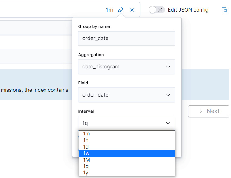
Figure 9.8 – Adjust the frequency of the date histogram from the dropdown
- Next, for our aggregation, let's choose the familiar avg(total_taxful_price). After we have made our selection, the Transform wizard will display a preview, which will show the average price paid by a customer per order, grouped by different weeks for a few sample rows. The purpose of the preview is to act as a checkpoint. Since transform jobs can be resource-intensive, at this stage it is good to pause and examine the preview to make sure the data is transformed into a format that you desire.
- Sometimes we might want to interrogate our data in ways that do not lend themselves to simple one-tiered group-by configurations like the one we explored in the preceding steps. It is possible to nest group-by configurations, as we will see in just a moment. Suppose that in our hypothetical e-commerce store example, we would also be interested in seeing the average amount of money spent by week and by geographic region.
To solve this, let's go back to the Transform wizard and add a second group-by field. In this case, we want to group by geoip.region_name. As before, the wizard shows us a preview of the transform once we select the group-by field. As in the previous case, it is good to take a moment to look at the rows displayed in the preview to make sure the data has been transformed in the desired way.
Tip
Click on the Columns toggle above the transform preview table to rearrange the order of the columns.
In addition to creating multiple group-by configurations, we can also add multiple aggregations to our transform. Suppose that in addition to the average amount of money spent per customer per week and per region, we would also be interested in finding out the number of unique customers who placed orders in our store. Let's see how we can add this aggregation to our transform.
- In the Aggregations drop-down menu in the wizard, scroll down until you find the entity cardinality (customer.full_name.keyword) and click on it to select it. The resulting aggregation will be added to your transform configuration and the preview should now display one additional column.
You can now follow the steps outlined in the tutorial of the previous section to assign an ID and a destination index for the transform, as well as to create and start the job. These will be left as exercises for you.
In the previous two sections, we examined the two key components of transforms: the pivot and aggregations, and did two different walk-throughs to show how both simple and advanced pivot and aggregation combinations can be used to interrogate our data for various insights.
While following the first transform, you may have noticed that in Figure 9.6, we left the Continuous mode checkbox unchecked. We will take a deeper look at what it means to run a transform in continuous mode in the next section.
Discovering the difference between batch and continuous transforms
The first transform we created in the previous section was simple and ran only once. The transform job read the source index kibana_sample_data_ecommerce, which we configured in the Transform wizard, performed the numerical calculations required to compute the average price paid by each customer, and then wrote the resulting documents into a destination index. Because our transform runs only once, any changes to our source index kibana_sample_data_ecommerce that occur after the transform job runs will no longer be reflected in the data in the destination index. This kind of transform that runs only once is known as a batch transform.
In many real-world use cases that produce records of transactions (like in our fictitious e-commerce store example), new documents are being constantly added to the source index. This means that our pivoted entity-centric index that we obtained as a result of running the transform job would be almost immediately out of date. One solution to keep the destination index in sync with the source index is to keep deleting the destination index and rerunning the batch transform job at regular intervals. This, however, is not practical and requires a lot of manual effort. This is where continuous transforms step in.
If we have a source index that is being updated and we want to use that to create a pivoted entity-centric index, then we have to use a continuous transform instead of a batch transform. Let's explore continuous transforms in a bit more detail to understand how they differ from batch transforms and what important configuration parameters should be considered when running a continuous transform.
First, let's set the stage for the problem we are trying to solve. Suppose we have a fictitious microblogging social media platform, where users post short updates, assign categories to the updates and interact with other users as well as predefined topics. It is possible to share a post and like a post. Statistics for each post are recorded as well. We have written some Python code to help generate this dataset. This code and accompanying instructions for how to run this code are available under the Chapter 9 - Introduction to Data Frame Analytics folder in the GitHub repository for this book (https://github.com/PacktPublishing/Machine-Learning-with-Elastic-Stack-Second-Edition/tree/main/Chapter%209%20-%20Introduction%20to%20Data%20Frame%20Analytics). After running the generator, you will have an index called social-media-feed that will contain a number of documents.
Each document in the dataset records a post that the user has made on the social media platform. For the sake of brevity, we have excluded the text of the post from the document. Figure 9.9 shows a sample document in the social-media-feed index.
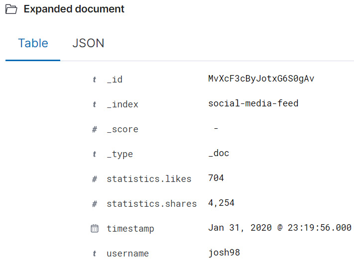
Figure 9.9 – A sample document in the social-media-feed index records the username, the time the post was submitted to the platform, as well as some basic statistics about the engagement the post received
In the next section, we will see how to use this fictional social media platform dataset to learn about continuous transforms.
Analyzing social media feeds using continuous transforms
In this section, we will be using the dataset introduced previously to explore the concept of continuous transforms. As we discussed in the previous section, batch transforms are useful for one-off analyses where we are either happy to analyze a snapshot of the dataset at a particular point in time or we do not have a dataset that is changing. In most real-world applications, this is not the case. Log files are continuously ingested, many social media platforms have around the clock activity, and e-commerce platforms serve customers across all time zones and thus generate a stream of transaction data. This is where continuous transforms step in.
Let's see how we can analyze the average level of engagement (likes and shares) received by a social media user using continuous transforms:
- Navigate to the Transforms wizard. On the Stack Management page, look to the left under the Data section and select Transforms.
- Just as we did in the previous sections, let's start by creating the transform. For the source index, select the social-media-feed index pattern. This should give you a view similar to the one in Figure 9.10.
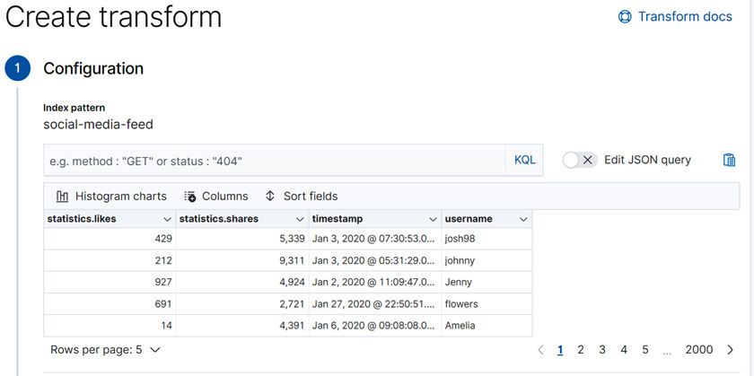
Figure 9.10 – The Transforms wizard shows a sample of the social-media-feed index
- In this case, we will be interested in computing aggregations of the engagement metrics of each post per username. Therefore, our Group by configuration will include the username, while our aggregations will compute the total likes and shares per user, the average likes and shares per user as well as the total number of posts each user has made. The final Group by and Aggregations configurations should look something like Figure 9.11.
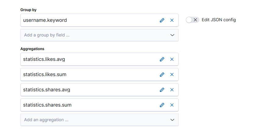
Figure 9.11 – Group by and Aggregations configuration for our continuous transform
- Finally, tick the Continuous mode selector and confirm that Date field is selected correctly as timestamp as shown in Figure 9.12.
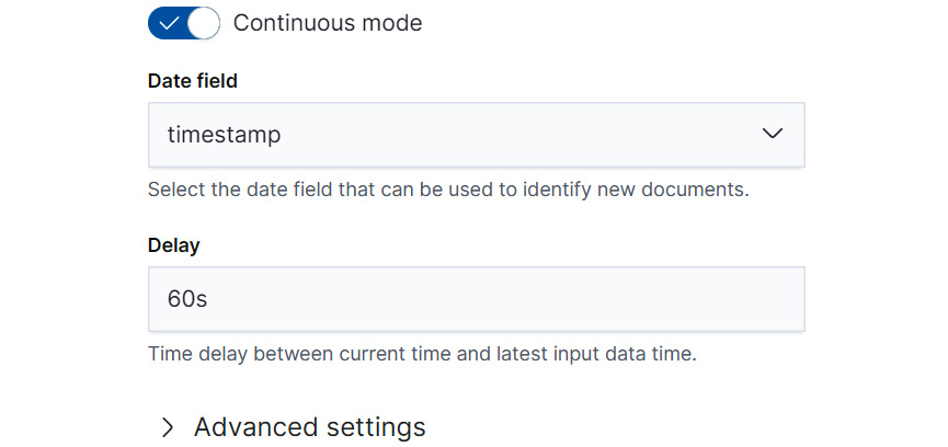
Figure 9.12 – Select Continuous mode to make sure the transform process periodically checks the source index and incorporates new documents into the destination index
- Once you click Create and start, you can return to the Transforms page and you will see the continuous transforms job for the social-media-feed index running. Note the continuous tag in the job description.

Figure 9.13 – Continuous transforms shown on the Transforms page. Note that the mode is tagged as continuous
- Let's insert some new posts into our index social-media-feed and see how the statistics for the user Carl change after a new document is added to the source index for the transform. To insert a new post, open the Kibana Dev Console and run the following REST API command (see chapter9 in the book's GitHub repository for a version that you can easily copy and paste into your own Kibana Dev Console if you are following along):
POST social-media-feed/_doc
{
"username": "Carl",
"statistics": {
"likes": 320,
"shares": 8000
},
"timestamp": "2021-01-18T23:19:06"
}
- Now, that we have added a new document into the source index social-media-feed, we expect that this document will be picked up by the continuous transform job and incorporated into our transform's destination index, social-media-feed-engagement. Figure 9.14 showcases the transformed entry for the username Carl.
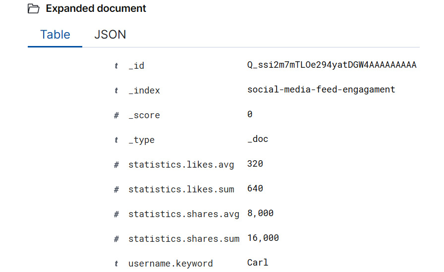
Figure 9.14 – The destination index of the continuous transform job holds an entry for the new username Carl, which we added manually through the Kibana Dev Console
The preceding example gives a very simplified walk-through of how continuous transforms work and how you can create your own continuous transform using the Transforms wizard available in Kibana. In Chapter 13, Inference, we will return to the topic of continuous transforms when we showcase how to combine trained machine learning models, inference, and transforms.
For now, we will take a brief detour into the world of the scripting language Painless. While the Transforms wizard and the many pre-built Group by and Aggregations configurations that it offers suffice for many of the most common data analysis use cases, more advanced users will wish to define their own aggregations. A common way to do this is with the aid of the Elasticsearch embedded scripting language, Painless.
In the next section, we will take a little tour of the Painless world, which will prepare you for creating your own advanced transform configurations.
Using Painless for advanced transform configurations
As we have seen in many of the previous sections, the built-in pivot and aggregation options allow us to analyze and interrogate our data in various ways. However, for more custom or advanced use cases, the built-in functions may not be flexible enough. For these use cases, we will need to write custom pivot and aggregation configurations. The flexible scripting language that is built into Elasticsearch, Painless, allows us to do this.
In this section, we will introduce Painless, illustrate some tools that are useful when working with Painless, and then show how Painless can be applied to create custom Transform configurations.
Introducing Painless
Painless is a scripting language that is built into Elasticsearch. We will take a look at Painless in terms of variables, control flow constructs, operations, and functions. These are the basic building blocks that will help you develop your own custom scripts to use with transforms. Without further ado, let's dive into the introduction.
It is likely that many readers of this book come from a sort of programming language background. You may have written data cleaning scripts with Python, programmed a Linux machine with bash scripts, or developed enterprise software with Java. Although these languages have many differences and are useful for different purposes, they all have shared building blocks that help human readers of the language understand them. Although there is an almost infinite number of approaches to teaching a programming language, the approach we will take here will be based on understanding the following basic topics about Painless: variables, operations (such as addition, subtraction, and various Boolean tests), control flow (if-else constructs and for loops) and functions. These are analogous concepts that users familiar with another programming language should be able to relate to. In addition to these concepts, we will be looking at some aspects that are particular to Painless, such as different execution contexts.
When learning a new programming language, it is important to have a playground that can be used to experiment with syntax. Luckily, with the 7.10 version of Elasticsearch, the Dev Tools app now contains the new Painless Lab playground, where you can try out the code samples presented in this chapter as well as any code samples you write on your own.
The Painless Lab can be accessed by navigating to Dev Tools as shown in Figure 9.15 and then, in the top menu of the Dev Tools page, selecting Painless Lab.
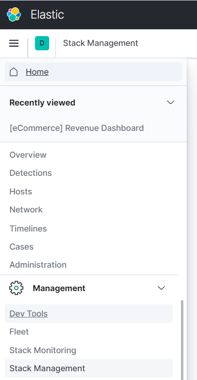
Figure 9.15 – The link to the Dev Tools page is located in the lower section of the Kibana side menu. Select it to access the interactive Painless lab environment
This will open an embedded Painless code editor as shown in Figure 9.16.
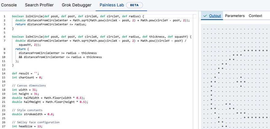
Figure 9.16 – The Painless Lab in Dev Tools features an embedded code editor. The Output window shows the evaluation result of the code in the code editor
The code editor in the Painless Lab is preconfigured with some sample functions and variable declarations to illustrate how one might draw the figure in the Output window in Figure 9.16 using Painless. For now, you can delete this code to make space for your own experiments that you will carry out as you read the rest of this chapter.
Tip
The full Painless language specification is available online here: https://www.elastic.co/guide/en/elasticsearch/painless/master/painless-lang-spec.html. You can use it as a reference and resource for further information about the topics covered later.
Variables, operators, and control flow
One of the first things we usually want to do in a programming language is to manipulate values. In order to do this effectively, we assign those values names or variables. Painless has types and before a variable can be assigned, it must be declared along with its type. The syntax for declaring a variable is as follows: type_identifier variable_name ;.
How to use this syntax in practice is illustrated in the following code block, where we declare variables a and b to hold integer values, the variable my_string to hold a string value, and the variable my_float_array to hold an array of floating values:
int a;
int b;
String my_string;
float[] my_float_array;
At this point, the variables do not yet hold any non-null values. They have just been initialized in preparation for an assignment statement, which will assign to each a value of the appropriate type. Thus, if you try copying the preceding code block into the Painless Lab code editor, you will see an output of null in the Output window as shown in Figure 9.17.

Figure 9.17 – On the left, Painless variables of various types are initialized. On the right, the Output panel shows null, because these variables have not yet been assigned a value
Important note
The Painless Lab code editor only displays the result of the last statement.
Next, let's assign some values to these variables so that we can do some interesting things with them. The assignments are shown in the following code block. In the first two lines, we assign integer values to our integer variables a and b. In the third line, we assign a string "hello world" to the string variable my_string, and in the final line, we initialize a new array with floating-point values:
a = 1;
b = 5;
my_string = "hello world";
my_double_array = new double[] {1.0, 2.0, 2.5};
Let's do some interesting things with these variables to illustrate what operators are available in Painless. We will only be able to cover a few of the available operators. For the full list of available operators, please see the Painless language specification (https://www.elastic.co/guide/en/elasticsearch/painless/current/painless-operators.html). The following code blocks illustrate basic mathematical operations: addition, subtraction, division, and multiplication as well as the modulus operation or taking the remainder:
int a;
int b;
a = 1;
b = 5;
// Addition
int addition;
addition = a+b;
// Subtraction
int subtraction;
subtraction = a-b;
// Multiplication
int multiplication;
multiplication = a*b;
// Integer Division
int int_division;
int_division = a/b;
// Remainder
int remainder;
remainder = a%b;
Try out these code examples on your own in the Painless Lab and you should be able to see the results of your evaluation, as illustrated in the case of addition in Figure 9.18.

Figure 9.18 – Using the Painless Lab code editor and console for addition in Painless. The result stored in a variable called "addition" in the code editor on the left is displayed in the Output tab on the right
In addition to mathematical operations, we will also take a look at Boolean operators. These are vital for many Painless scripts and configurations as well as for control flow statements, which we will take a look at afterward.
The code snippets that follow illustrate how to declare a variable to hold a Boolean (true/false) value and how to use comparison operators to determine whether values are less, greater, less than or equal, or greater than or equal. For a full list of Boolean operators in Painless, please consult the Painless specification available here: https://www.elastic.co/guide/en/elasticsearch/painless/current/painless-operators-boolean.html:
boolean less_than = 4<5;
boolean greater_than = 4>5;
boolean less_than_or_equal = 4 <=5;
boolean greater_than_or_equal = 4 >= 5;
As an exercise, copy the preceding code block into the Painless Lab code editor. If you wish, you can view the contents of each of these variables by typing its name followed by a semicolon into the last line of the Painless Lab code editor and the value stored in the variable will be printed in the Output window on the right, as shown in Figure 9.19.
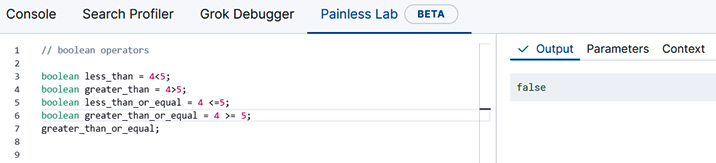
Figure 9.19 – Typing in the variable name followed by a semicolon in the Painless Lab code editor will output the contents of the variable in the Output tab
While the Boolean operator illustrated here is useful in many numerical computations, we probably could not write effective control flow statements without the equality operators == and !=, which check whether or not two variables are equal. The following code block illustrates how to use these operators with a few practical examples:
// boolean operator for testing for equality
boolean two_equal_strings = "hello" == "hello";
two_equal_strings;
// boolean operator for testing for inequality
boolean not_equal = 5!=6;
not_equal;
Last but not least in our tour of the Boolean operators in Painless, we will look at a code block that showcases how to use the instanceof operator, which checks whether a given variable is an instance of a type and returns true or false. This is a useful operator to have when you are writing Painless code that you only want to operate on variables of a specified type:
// boolean operator instanceof tests if a variable is an instance of a type
// the variable is_integer evaluates to true
int int_number = 5;
boolean is_integer = int_number instanceof int;
is_integer;
In the final part of this section, let's take a look at one of the most important building blocks in our Painless script: if-else statements and for loops. The syntax for if-else statements is shown in the following code block with the help of an example:
int a = 5;
int sum;
if (a < 6){
sum = a+5;
}
else {
sum = a-5;
}
sum;
In the preceding code block, we declare an integer variable, a, and assign it to contain the integer value 5. We then declare another integer variable, sum. This variable will change according to the execution branch that is taken in the if-else statement. Finally, we see that the if-else statement first checks whether the integer variable a is less than 6, and if it is, stores the result of adding a and the integer 5 in the variable sum. If not, the amount stored in the variable sum is the result of subtracting 5 from a.
If you type this code in the Painless Lab code editor, the Output console will print out the value of sum as 10 (as shown in Figure 9.20), which is what we expect based on the previous analysis.
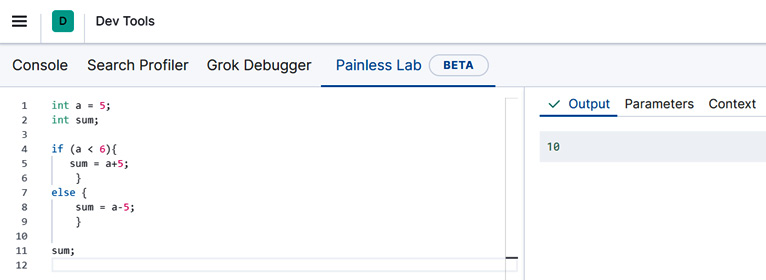
Figure 9.20 – The if-else statement results in the sum variable being set to the value 10
Finally, we will take a look at how to write a for loop, which is useful for various data analysis and data processing tasks with Painless. In our for loop, we will be iterating over a string variable and calculating how many occurrences of the letter a occur in the string. This is a very simple example, but will hopefully help you to understand the syntax so that you can apply it in your own examples:
// initialize the string and the counter variable
String sample_string = "a beautiful day";
int counter = 0;
for (int i=0;i<sample_string.length();i++){
// get a letter from the string using the substring method
String letter = sample_string.substring(i, i+1);
//use an if-statement to check if the current letter being processed is an a
if (letter=="a") {
// is yes, increment the counter
counter++
}
}
counter;
Copy and paste this code sample (a copy can be found in the GitHub repository https://github.com/PacktPublishing/Machine-Learning-with-Elastic-Stack-Second-Edition for this book under the folder Chapter 9 - Introduction to Data Frame Analytics) into your Painless Lab and you will see that the counter variable in the Output panel will print out 3, as we expect, since there are three occurrences of the letter "a" in the string "a beautiful day."
Functions
Now that we have covered variables, operators, and control flow statements, let's turn our attention for a moment to functions. Sometimes, we might notice ourselves writing the same lines of code over and over again, across multiple different scripts and configurations. At this point, it might be more economical to package up the lines that we find ourselves reaching for over and over again into a reusable piece of code that we can reference with a name from our Painless scripts.
Let's return to the example where we wrote a for loop with an if statement to calculate the instances of the letter "a" in a given string. Suppose we want to reuse this functionality and make it slightly more generic. This is a perfect opportunity to package up this piece of code as a Painless function.
There are three parts to writing a function in Painless. First, we write the function header, which specifies the type of the value the function returns, as well as the name of the function. This is what we will use to refer to the function when we use it in our scripts or Ingest Pipelines, which we will discuss in more detail when we discuss Inference in Chapter 13, Inference. The skeleton of our function, which we will call letterCounter, is shown in the following code block:
int letterCounter(){
}
The int in front of the function name determines the type of value returned by this function. Since we are interested in the number of occurrences of a particular letter in a particular string, we will be returning an integer count. The parentheses after the name letterCounter will hold the parameters that the function accepts. For now, we have not specified any parameters, so there is nothing between the parentheses. Finally, the two curly braces signify the place for the function body – this is where all of the logic of the function will reside.
Now that we have investigated the elements that go into creating a basic function header, let's populate the function body (the space between the curly braces with the code we wrote in the previous section while learning about for loops). Our function now should look something like the following code block:
int letterCounter(){
// initialize the string and the counter variable
String sample_string = "a beautiful day";
int counter = 0;
for (int i=0;i<sample_string.length();i++){
// get a letter from the string using the substring method
String letter = sample_string.substring(i, i+1);
//use an if-statement to check if the current letter being processed is an a
if (letter=="a") {
// is yes, increment the counter
counter++
}
}
return counter;
}
letterCounter();
If you look toward the end of the function body, you will notice that the only difference between our for loop residing inside the function body is that now we have added a return statement. This allows our value of interest stored in the variable counter to be returned to the code calling the function, which brings us to our next question. Now that we have written our first Painless function and it does something interesting, how do we go about calling this function?
In the Painless Lab environment, we would simply type out letterCounter(); as shown in Figure 9.21. The result returned by this function is, as we expect based on our previous dissection of this code sample, 3.

Figure 9.21 – The definition of the sample function letterCounter displayed alongside an example of how to call a function in the Painless Lab environment
Now that we have a working function, let's talk about making this function a bit more generic, which is what you will often need to do when working with either transforms, which we have been discussing in this chapter, or various ingest pipelines and script processors, which we will be discussing in Chapter 13, Inference. As it currently stands, our function letterCounter is very specific. It only computes the number of occurrences of a very specific letter – the letter a – in a very specific string, the phrase "a beautiful day."
Suppose that to make this snippet of code really useful, we would like to vary both the phrase and the letter that is counted. With functions, we can do this with minimal code duplication, by configuring function parameters. Since we want to vary both the letter and the phrase, let's make those two into function parameters. After the change, our function definition will look as in the following code block:
int letterCounter(String sample_string, String count_letter){
// initialize the string and the counter variable
int counter = 0;
for (int i=0;i<sample_string.length();i++){
// get a letter from the string using the substring method
String letter = sample_string.substring(i, i+1);
//use an if-statement to check if the current letter being processed is an a
if (letter==count_letter) {
// is yes, increment the counter
counter++
}
}
return counter;
}
Notice that now, in between the parentheses in the function header, we have defined two parameters: one sample_string parameter representing the phrase in which we want to count the occurrences of the second parameter, count_letter.
To call this function, we will first define new variables to hold our phrase ("a beautiful day," once again) and our letter of interest – this time the letter "b" instead of "a." Following this, we will pass both of these variables into the function call as shown in the following code block:
String phrase = "a beautiful day";
String letter_of_interest = "b";
letterCounter(phrase, letter_of_interest);
Since there is only one occurrence of the letter "b" in our phrase of interest, we will expect the result of executing this function to be 1, as is the case in Figure 9.22.
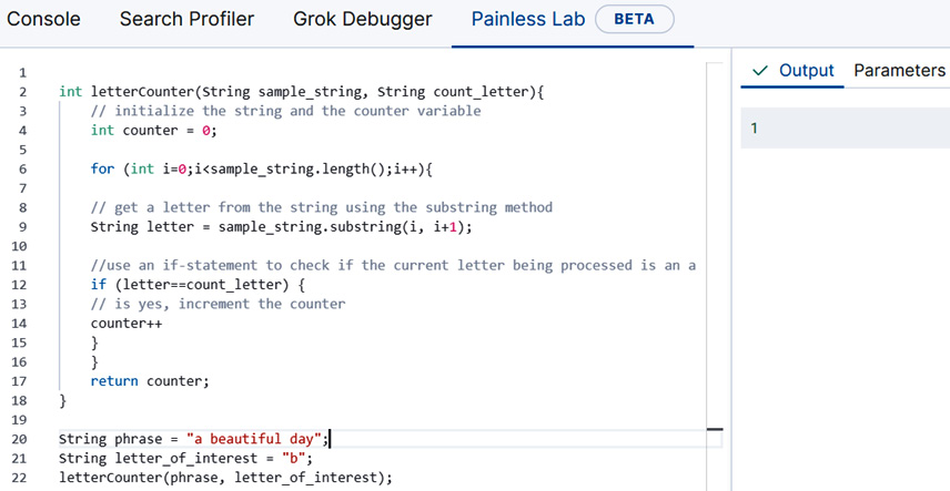
Figure 9.22 – The result of calling the function is shown in the Output panel on the right
Now you should be equipped to write your own Painless code! This will come in handy in Chapter 13, Inference, where we will use advanced Painless features to perform feature extractions and to write script processors.
Working with Python and Elasticsearch
In recent years, Python has become the dominant language for many data-intensive projects. Fueled by its easy-to-use machine learning and data analysis libraries, many data scientists and data engineers are now heavily relying on Python for most of their daily operations. Therefore, no discussions of machine learning in the Elastic Stack would be complete without exploring how a data analysis professional can work with the Elastic Stack in Python.
In this section, we will take a look at the three official Python Elasticsearch clients, understand the differences between them, and discuss when one might want to use one over the others. We will demonstrate how usage of Elastic Stack ML can be automated by using Elasticsearch clients. In addition, we will take a deeper look at Eland, the new data science native client that enables efficient in-memory data analysis backed by Elasticsearch. After exploring how Eland works, we will illustrate how Eland can be combined with Jupyter notebooks, an open source interactive data analysis environment to analyze data stored in Elasticsearch.
A brief tour of the Python Elasticsearch clients
Anyone who has used the Kibana Dev Tools Console to communicate with Elasticsearch knows that most things are carried out via the REST API. You can insert, update, and delete documents by calling the right endpoint with the right parameters. Not surprisingly, there are several levels of abstraction at which a client program calling these REST API endpoints can be written. The low-level client elasticsearch-py (https://elasticsearch-py.readthedocs.io/en/v7.10.1/) provides a thin Python wrapper on the REST API calls that one would normally execute through the Kibana Dev Console or through some application capable of sending HTTP requests. The next level of abstraction is captured by the Elasticsearch DSL client (https://elasticsearch-dsl.readthedocs.io/en/latest/). Finally, the most abstracted client is Eland (https://eland.readthedocs.io/en/7.10.1b1/), where the data frame, a tabular representation of data, is a first-class citizen. We will see in subsequent examples what this means for data scientists wishing to use Eland with Elasticsearch.
In addition to the available Elasticsearch clients, we are going to take a moment to discuss the various execution environments that are available to any data engineers or data scientists wishing to work with Python and Elasticsearch. This, in turn, will lead us to an introduction to Jupyter notebooks and the whole Jupyter ecosystem, which is a tool to know for anyone wishing to work with machine learning and the Elastic Stack.
The first and probably most familiar way to execute a Python program is to write our program's logic in a text file – or a script – save it with a .py extension to signify that it contains Python code, and then invoke the script using the command line as shown in Figure 9.23.

Figure 9.23 – One way to work with Python is to store our program in a text file or a script and then execute it from the command line
The second way is to use the interactive Python REPL, which is shown in Figure 9.24. Invoking python (or python3) on our command line will launch an interactive Python environment where we can write functions, define variables, and execute all sorts of Python code. While this environment is useful for small-scale or quick experiments, in practice it would be hard to work on a long-term or larger collaborative data analysis project in the REPL environment. Therefore, for most projects involving Python, data analysis, and the Elastic Stack, the environment of choice is some sort of integrated development environment that provides a code editor along with various tools to support both programming and execution.
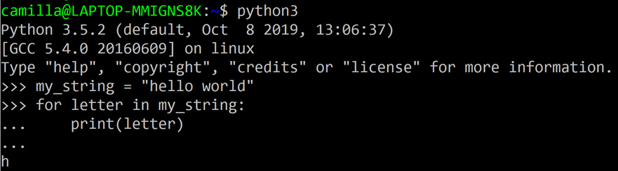
Figure 9.24 – A screenshot depicting a sample Python interactive shell or REPL, which is perfect for quick experiments in the Python programming language
A development environment that is specifically designed with data analysis in mind is a Jupyter notebook, which is illustrated in Figure 9.25.

Figure 9.25 – A sample Jupyter notebook
The notebook can be installed in a Python installation through a central package management service such as pip and is launched by typing jupyter notebook on the command line. The launched environment runs in a browser such as Chrome or Firefox and provides an environment where code snippets, text paragraphs, graphs, and visualizations (both interactive and static) can live side by side. Many authors have covered the Jupyter Notebook and the library ecosystem that exists around it much better than what we have space or time for in this chapter and thus we encourage those readers who want to or anticipate working more at the intersection of data analysis, Elasticsearch, and Python to take a look at the materials listed in the Further reading section at the end of this chapter.
Understanding the motivation behind Eland
Readers of the previous section might wonder, what was the motivation of building yet another Elasticsearch Python client when the community already has two clients to choose from? Moreover, why build an entire software library around the idea of a Data Frame object? The answers to both of these questions could probably fill an entire book, so the answers presented here will necessarily leave some subtleties unexplored. Nevertheless, we hope that for the interested reader, the discussion in this section will give some interesting context into how Eland came to be and why it was designed around the idea of the Data Frame.
Although Python appears to be the dominant force for many domains of data analysis and machine learning today, this was not always the case. In particular, in the early 2010s, the ecosystem was dominated by the statistical processing language R, which had a very useful construct – a dataframe object that allowed one to analyze rows of data in a table-like structure (a concept that is no doubt familiar to users of Excel). At about the same time, Wes McKinney, then working at the New York financial firm AQR Capital, started working on a library to make the lives of Python data analysts easier. This work culminated in the release of pandas, an open source data analysis library that is used by thousands of data scientists and data engineers.
One of the key features that made pandas useful and easy to use was the DataFrame object. Analogous to the R object, this object made it straightforward to manipulate and carry out analyses on data in a tabular manner. Although pandas is very powerful and contains a multitude of built-in functions and methods, it begins to hit limitations when the dataset one wishes to analyze is too large to fit in memory.
In these cases, data analysts often resort to sampling data from the various databases, for example, Elasticsearch, where it is stored, exporting it into flat files, and then reading it into their Python process so that it can be analyzed with pandas or another library. While this approach certainly works, the workflow would become more seamless if pandas were to interface directly with the database. What if we could transparently interface a DataFrame object with Elasticsearch so that the data analyst could focus on analyzing data instead of having to worry about managing the connection and exporting data from Elasticsearch? This is the very grounding idea of Eland. Hopefully, the next sections will demonstrate how this philosophy has materialized concretely in the design of this library.
Taking your first steps with Eland
Since Eland is a third-party library, you will first have to install it so that your Python installation is able to use it. The instructions for this across various operating systems are given under Chapter 9 - Introduction to Data Frame Analytics in the GitHub repository for this book: https://github.com/PacktPublishing/Machine-Learning-with-Elastic-Stack-Second-Edition/tree/main/Chapter%209%20-%20Introduction%20to%20Data%20Frame%20Analytics. We will assume that readers wishing to follow along with the material in this section of the book will have followed the instructions linked to complete the installation of the library. The examples and screenshots in this chapter will be illustrated using a Jupyter notebook environment, but it is also possible to run the code samples presented in this chapter in a standalone environment (for example, from a Python REPL or from a Python script). Examples that specifically require the Jupyter notebook environment will be clearly indicated:
- The first step that we have to do to make use of Eland is to import it into our environment. In Python, this is done using the import statement as shown in Figure 9.26. Note that when using a library such as Eland, it is common to assign an alias to the library. In the code snippet shown in Figure 9.26, we have assigned eland the alias ed using the keyword as. This will save us some typing in the future as we will be invoking the library name many times as we access its objects and methods.

Figure 9.26 – Importing Eland into the notebook
- After importing the code into our Jupyter notebook, we are free to start exploring. Let's start with the most basic things one can do with Eland: creating an Eland DataFrame. To create the DataFrame, we need to specify two things: the URL of our Elasticsearch cluster (for example, localhost if we are running Elasticsearch locally on the default port 9200) and the name of the Elasticsearch index. These two parameters are passed into the DataFrame constructor as shown in Figure 9.27.

Figure 9.27 – Creating a DataFrame in Eland involves the URL of the Elasticsearch cluster and the name of the index that contains the data we wish to analyze
- One of the first tasks we are interested in doing when we start examining a new dataset is learning what the data looks like (usually, it is enough to see a few example rows to get the general gist of the data) and some of the general statistical properties of the dataset. We can learn the former by calling the head method on our Eland DataFrame object as is shown in Figure 9.28.

Figure 9.28 – Calling the head method on the Eland DataFrame object will show us the first 5 rows in the dataset
- Knowledge of the latter, on the other hand, is obtained by calling the describe method, which will be familiar to pandas users and is shown in Figure 9.29.

Figure 9.29 – "describe" summarizes the statistical properties of the numerical columns in the dataset
- In addition to obtaining a basic overview of the dataset, we can easily access individual values of a given field in the index by using the get command in conjunction with the name of the field as shown in Figure 9.30.
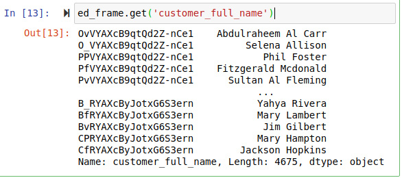
Figure 9.30 – We can work with the individual field values in the index by using the get method
- Finally, we can compute aggregations on our numerical columns using the aggregate method. In the example illustrated in Figure 9.31, we select two numerical columns total_unique_products and taxful_total_price, and compute the sum, the minimum, and the maximum of the values in these fields across all documents in the index.
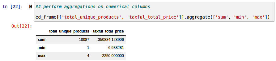
Figure 9.31 – Computing aggregations on selected columns is possible in Eland using the aggregate method
While the steps illustrated here are relatively simple, we hope that they've showcased how seamlessly it is possible to integrate Elasticsearch, working in Python, and a data analysis environment such as the Jupyter Notebook into one, seamless data analysis workflow. We will build upon this foundation with Eland further in Chapter 13, Inference, when we will take a look at more advanced use cases.
Summary
In this section, we have dipped our toes into the world of Data Frame Analytics, a whole new branch of machine learning and data transformation tools that unlock powerful ways to use the data you have stored in Elasticsearch to solve problems. In addition to giving an overview of the new unsupervised and supervised machine learning techniques that we will cover in future chapters, we have studied three important topics: transforms, using the Painless scripting language, and the integration between Python and Elasticsearch. These topics will form the foundation of our future work in the following chapters.
In our exposition on transforms, we studied the two components – the pivot and aggregations – that make up a transform, as well as the two possible modes in which to run a transform: batch and continuous. A batch transform runs only once and generates a transformation on a snapshot of the source index at a particular point in time. This works perfectly for datasets that do not change much or when the data transformation needs to be carried out only at a specific point in time. For many real-world use cases, such as logging or our familiar e-commerce store example, the system being monitored and analyzed is constantly changing. An application is constantly logging the activities of its users, an e-commerce store is constantly logging new transactions. Continuous transforms are the tools of choice for analyzing such streaming datasets.
While the pre-configured options available in the Transform wizard we showcased in our examples are suitable for most situations, more advanced users may wish to configure their own aggregations. In order to do this (and in general, in order to be able to perform many of the more advanced configurations we will discuss in later chapters), users need to be familiar with Painless, the scripting language that is embedded in Elasticsearch. In particular, we took a look at how to declare variables in Painless, how to manipulate those variables with operations, how to construct more advanced programs using control flow statements, and finally how to package up useful code snippets as functions. All of these will be useful in our explorations in later chapters!
Last but not least, we took a whirlwind tour of how to use Python when analyzing data stored in Elasticsearch. We took a look at the two existing Python clients for Elasticsearch, elasticsearch-py and elasticsearch-dsl and laid the motivation behind the development of the third and newest client, Eland.
In the next section, we will dive into the first of the three new machine learning methods added into the Elastic Stack: outlier detection.
Further reading
For more information on the Jupyter ecosystem and, in particular, the Jupyter Notebook, have a look at the comprehensive documentation of Project Jupyter, here: https://jupyter.org/documentation.
If you are new to Python development and would like to have an overview of the language ecosystem and the various tools that are available, have a look at the Hitchiker's Guide to Python, here: https://docs.python-guide.org/.
To learn more about the pandas project, please see the official documentation here: https://pandas.pydata.org/.
For more information on the Painless embedded scripting language, please see the official Painless language specification, here: https://www.elastic.co/guide/en/elasticsearch/painless/current/painless-lang-spec.html.