Chapter 12: Regression
In the previous chapter, we studied classification – one of the two supervised learning techniques available in the Elastic Stack. However, not all real-world applications of supervised learning lend themselves to the format required for classification. What if, for example, we wanted to predict the sales prices of apartments in our neighborhood? Or the amount of money a customer will spend in our online store? Notice that the value we are interested in here is not a discrete class, but instead is a value that can take a variety of continuous values in a range.
This is exactly the problem solved by regression analysis. Instead of predicting which class a given datapoint belongs to, we can predict a continuous value. Although the end goal is slightly different than that in classification, the underlying algorithm that is used for regression is the same as the one we examined for classification in the previous chapter. Thus, we already know a lot about how regression works from the foundations we built in Chapter 11, Classification Analysis
Because the result of regression is continuous values instead of a discrete class label like in the case of classification, the ways in which we evaluate the performance of a regression model are slightly different than the ways we examined for classification in the previous chapter. Instead of using confusion matrices and various metrics computed from the number of correctly labeled and mislabeled examples, we compute aggregate metrics that capture how far the continuous values predicted for our dataset are from the actual values in our dataset. We will take a closer look at how this works in practice and what measures are used later in this chapter.
In this chapter, we will cover the following topics:
- Using regression to predict house prices in a geographic location
- Understanding how decision trees can be applied to create regression models
Technical requirements
The material in this chapter will require an Elasticsearch cluster running version 7.10.1 or later. Some examples may include screenshots or guidance about details that are only available in later versions of Elasticsearch. In such cases, the text will explicitly mention which later version is required to run the example.
Using regression analysis to predict house prices
In the previous chapter, we examined the first of the two supervised learning methods in the Elastic Stack – classification. The goal of classification analysis is to use a labeled dataset to train a model that can predict a class label for a previously unseen datapoint. For example, we could train a model on historical measurements of cell samples coupled with information about whether or not the cell was malignant and use this to predict the malignancy of previously unseen cells. In classification, the class or dependent variable that we are interested in predicting is always a discrete quantity. In regression, on the other hand, we are interested in predicting a continuous variable.
Before we examine the theoretical underpinnings of regression a bit closer, let's dive right in and do a practical walk-through of how to train a regression model in Elasticsearch. The dataset we will be using is available on Kaggle (https://www.kaggle.com/harlfoxem/housesalesprediction) and describes the prices of houses sold in an area of Washington State in the United States between 2014 and 2015. The original dataset has been modified slightly to make it easier to ingest into Elasticsearch and is available in the book's GitHub repository here (https://github.com/PacktPublishing/Machine-Learning-with-Elastic-Stack-Second-Edition/blob/main/Chapter%2012%20-%20Regression%20Analysis/kc_house_data_modified.csv). We will get started as follows:
- Ingest the dataset into Elasticsearch using your preferred method. If you wish, you can use the Upload file functionality available in the Machine Learning app's Data Visualizer as shown in Figure 12.1:
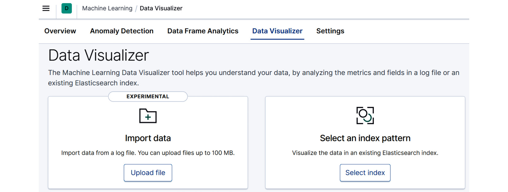
Figure 12.1 – The Upload file functionality in the Machine Learning app's Data Visualizer
- Once we have ingested this data, let's take a moment to examine it in the Machine Learning app's Data Visualizer. In this view, we can see at a glance what fields are present in the data and what the distribution of values is for each field. For example, for our house price dataset, we can see in a histogram visualization of the price values in Figure 12.2 that most house prices in this dataset fall between 200,000 USD and 900,000 USD, with a small minority of houses selling for more than 900,000 USD:
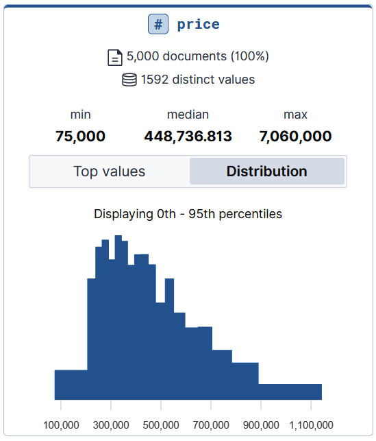
Figure 12.2 – The distribution of values for the price field as shown in Data Visualizer
Looking at data values and distributions in Data Visualizer can quickly alert us to potential problems, such as invalid or missing values in a given field, with a dataset.
Next, let's navigate to the Data Frame Analytics wizard. In the left-hand side sliding menu in Kibana, click on Machine Learning to navigate to the Machine Learning app's main page. On this page, in the Data Frame Analytics jobs section, if you have not yet created a Data Frame Analytics job, click on the Create job button. If you have, first click on the Manage jobs button. This will take you to the Data Frame Analytics page, where you will find a list of existing Data Frame Analytics jobs (for example, if you had created any from following the walk-throughs in the previous chapters) and the Create job button.
This will take you to the Data Frame Analytics wizard that we have already seen in Chapter 10, Outlier Detection, as well as in Chapter 11, Classification Analysis.
- Once you have selected your source index pattern (this should match the name of the index pattern you selected when importing or uploading the data in step 1), select Regression from the Data Frame Analytics wizard's job type selector as shown in Figure 12.3:
Figure 12.3 – Select Regression as the job type in the Data Frame Analytics job wizard selector
- Next, let's configure the Dependent Variable selector and the fields that are going to be included in our analysis. As you might recall from previous chapters, the dependent variable denotes the field that contains the labels that we wish to use to train our supervised model. For classification problems, this field was the one that contained the labels of the class to which a given datapoint belonged (see Chapter 11, Classification Analysis, for more information). For regression, this field will contain the continuous values that we wish to train our model to predict. In this case, we wish to predict the price of a house and we thus select the price field.
After selecting the dependent variable, let's move on to selecting the fields that are going to be included or excluded from our analysis. While many of the fields in the dataset provide useful information for predicting the value of the dependent variable (price), there are a few fields that we know from the beginning will not correlate with the price and thus should be removed. The first of these is the ID (id) of the datapoint. It is simply a row number denoting the position of the datapoint in the original data file and thus is not expected to carry useful information. In fact, including it could result in more harm than good. For example, if the original data file were organized in such a way that all low-priced houses were situated at the beginning of the file with low id numbers and all high-priced houses at the end of the file, the model might consider the id datapoint important in determining the price of the house even though we know that this is nothing but an artifact of the dataset. This, in turn, would be detrimental to the model's performance on future, yet-unseen datapoints. If we assume that the id value of the datapoints is growing, any new datapoint added to the dataset would automatically have a higher id number than any datapoint in the training data and would thus lead to the model assuming that any new datapoint has a higher price.
Additionally, we will also exclude information about the latitude and the longitude of the house's location, since these variables cannot be interpreted as geographic locations by the machine learning algorithm and would thus be simply interpreted as numbers. The final configuration should look like Figure 12.4:

Figure 12.4 – Fields that are not included in the analysis
- After configuring the dependent variable and the included and excluded fields, we can move on to the additional configuration items. While we will leave most of the values in this section set to the defaults, we will change the number for Feature importance values from 0 to 4. If set to 0, no feature importance values are written out. When set to 4, four of the most important feature values are written out for each datapoint. As briefly discussed in Chapter 11, Classification Analysis, feature importance values are written out separately for each document and help to determine why the model classified a particular document in a particular way. We will return to this point slightly later in the chapter:

Figure 12.5 – Feature importance values configuration
We leave the rest of the settings on the defaults and start running the job by scrolling to the bottom of the wizard and clicking the Create and start button.
- After completing the steps in the wizard and creating and starting your job, navigate back to the Data Frame Analytics page. This will show you an overview of all of the Data Frame Analytics jobs you have created, including the regression job we created in the preceding steps. Once the job has completed, click on the menu on the right-hand side and click on View as shown in Figure 12.6:

Figure 12.6 – Select View to see the results for the Data Frame Analytics job
This will take us to the Exploration page, which allows us to explore various metrics of the newly trained regression model. The first thing that requires attention on this page is the Training/Testing dataset toggle, which is displayed in Figure 12.7:
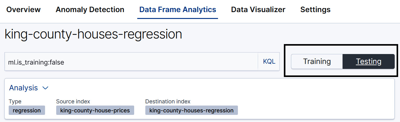
Figure 12.7 – The Training/Testing toggle in the Data Frame Analytics results viewer
It is important to keep this toggle in mind when viewing the metrics on the Exploration page, because the evaluation metrics of the model mean different things depending on which of the metrics is selected. In this case, we are interested in how the model will perform when it is trying to make predictions on previously unseen datapoints. The dataset that most closely approximates this is the testing dataset – in other words, the dataset that was not used in the training process.
- Let's scroll down and take a look at the Model evaluation metrics for the testing dataset, which is shown in Figure 12.8:
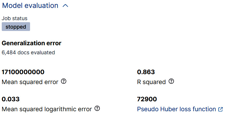
Figure 12.8 – The generalization error
We will take a more detailed look at what each of these metrics means later in the chapter, but for now you can treat them as aggregate measures of how close the model's predictions of the house prices were to the actual house prices.
- Finally, what might be of interest to many users is which of the fields in our dataset were most important in determining the final prediction of the model. We can see this by taking a look at the Total feature importance section on the Exploration page as shown in Figure 12.9:
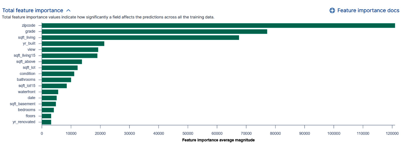
Figure 12.9 – The total feature importance
As we can see from the figure, the most important factor in determining the sales price of a house in King Country in Washington State is zip code, or the location of the house. Among the least important factors are the year the house was renovated, yt_renovated, and the number of floors (floors) it has.
It is good to keep in mind that the features shown in this diagram are the most important features across the whole dataset. The features that determine the sales price of an individual datapoint in the dataset can, however, be very different. A bit earlier in this walk-through, during the creation of the job in the Data Frame Analytics wizard, we configured Feature importance values to be 4. This means that after the model has been trained, the four most important feature importance values will be written out to the results index. Let's take a look at a sample document in our results index, king-county-houses-regression. This document is shown in Figure 12.10:
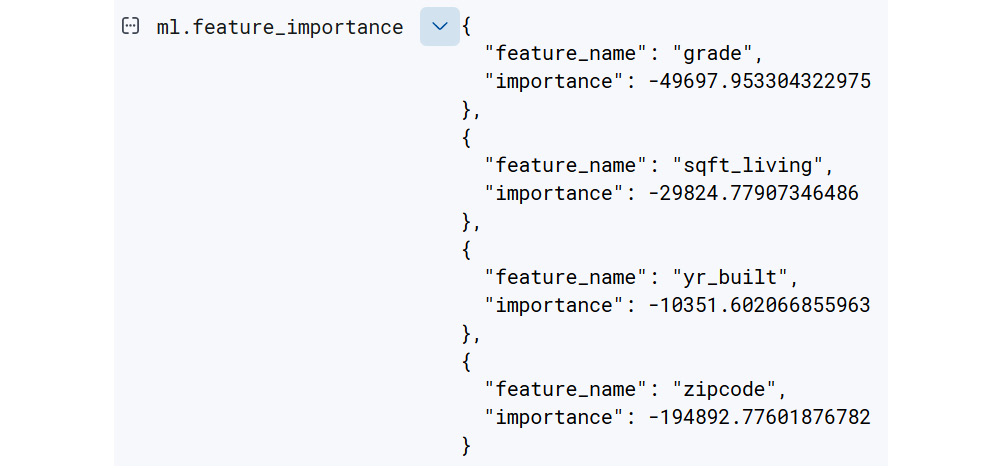
Figure 12.10 – Feature importance values for a sample document in the results index
As we can see in Figure 12.10, for this particular house, the four most important feature values are grade, sqft_living (the amount of living space in the house measured in square feet), yr_built (the year the house was built), and zipcode (a numerical representation of the location of the house). One thing to note is that all of the feature importance values here are negative, which means that they contribute to lowering the price of the house.
Let's take a look at the top four feature importance values in another document (shown in Figure 12.11) in the results index and compare them to the previous feature importance values to see how much variation there can be:

Figure 12.11 – The four most important features for determining the price of this house
As we can see, the house represented by the document in Figure 12.11 shares some features with the house in Figure 12.10 but also has some unique ones. In addition, the feature importance values for this house affect its price positively.
Now that you have briefly seen how to train a regression model and evaluate its results, a natural question to ask is, what next? If you were using this model for a real-world use case, such as to predict the potential house prices of yet-unsold houses in King County or another geographic location, you could use inference to examine and deploy this model. This will be covered in greater detail in Chapter 13, Inference. In the next section, we will briefly return to our discussion of decision trees that we began in Chapter 11, Classification Analysis, and see how the ideas we developed in that chapter apply to regression problems.
Using decision trees for regression
As we have discussed in the preceding chapters, regression is a supervised learning technique. As discussed in Chapter 11, Classification Analysis, the goal of supervised learning is to take a labeled dataset (for example, a dataset that has features of houses and their sales price – the dependent variable) and distill the knowledge in this data into an artifact known as a trained model. This trained model can then be used to predict the sales prices of houses that the model has not previously seen. When the dependent variable that we are trying to predict is a continuous variable, as opposed to a discrete variable, which is the domain of classification, we are dealing with regression.
Regression – the task of distilling the information presented in real-world observations or data – is a field of machine learning that encompasses techniques far broader than the decision tree technique that is used in Elasticsearch's Machine learning functionality. However, we will limit ourselves here to a conceptual discussion of how regression can be carried out using decision trees (a simplified version of the process that takes place inside the Elastic Stack) and refer readers interested in learning more about regression to the literature. For example, the book Mathematics for Machine Learning (https://mml-book.github.io/) has a good introduction to regression.
In Chapter 11, Classification Analysis, we started our discussion of decision trees when applied to classification problems with a conceptual introduction of a flowchart that you might construct if you wanted to take houses and try and deduce what their sales price would be. An example fictional flowchart that you might construct is presented in Figure 12.12:
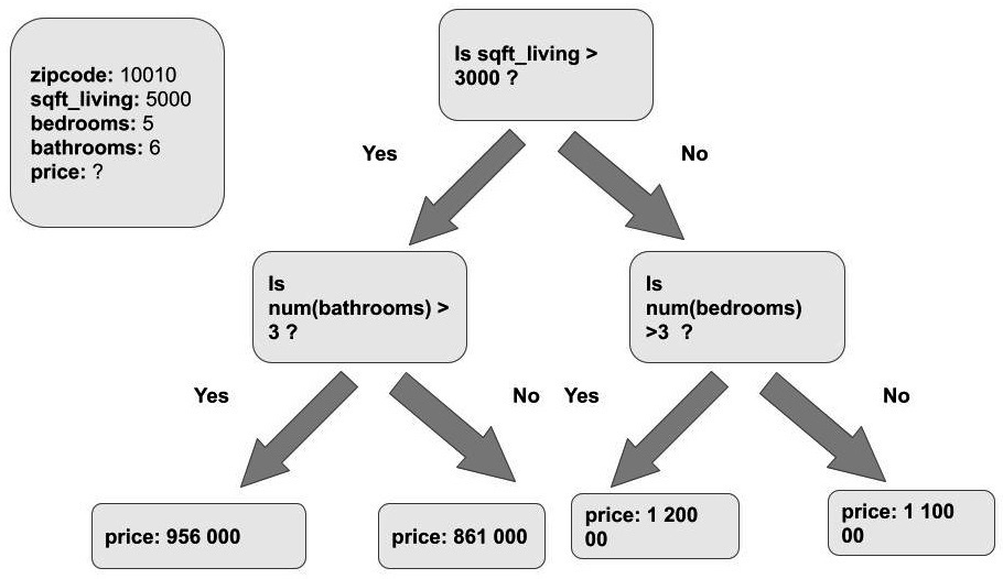
Figure 12.12 – A sample flowchart that illustrates the decisions that you might make to try to predict the sales price of a house
In the fictional flowchart shown in Figure 12.12, we have a sample house depicted by the box in the upper left-hand corner. This house has 5,000 square feet of living space, 5 bedrooms, and 5 bathrooms. We would like to predict the final sales price of the house based on these attributes and we are going to use the flowchart to help us. The way we do this in practice is we start at the top of the flowchart (or the root of the decision tree) and work our way downward toward the terminal nodes (the nodes that are not connected to any downstream nodes). Our sample house has a living area of 5,000 square feet, so we reply Yes for the first node and Yes again for the second child node. This leads to a terminal or a leaf node that contains the predicted price of our house: 956,000 USD.
A natural question to ask is, how do we create a flowchart like the one in Figure 12.12? There are two ingredients required to create this flowchart (or decision tree): the labeled dataset, which contains features of each house and its sales price, and the training algorithm, which will take this dataset and use it to construct a populated flowchart or decision tree that can then be used to make price predictions for previously unseen houses (this is done using inference, which is covered in detail in Chapter 13, Inference).
The process of training a decision tree based on a labeled dataset involves creating nodes like the ones depicted in Figure 12.12. These nodes split the dataset into progressively smaller and smaller subsets until we reach a situation where each subset fulfills certain criteria. In the case of classification, the process of progressively splitting the training dataset is stopped when the subsets reach a certain purity. This can be measured using several different metrics that capture the proportion of datapoints that belong to a certain class in a node. The purest node is the kind that contains only datapoints belonging to a certain class.
Since regression deals with continuous values, we cannot use purity as a measure to determine when to stop recursively splitting the dataset. Instead, we have another measure known as the loss function. A sample loss function for regression is the mean squared error. This measure captures how far the values predicted for the points falling in each node are from the actual errors.
Finally, if were cursively split the dataset many times, we end up with a simplified decision tree as depicted in Figure 12.13:

Figure 12.13 – A simplified trained decision tree. The leaf nodes contain several datapoints
As we see in Figure 12.13, at the end of the training process the terminal node leaves contain several datapoints each.
Summary
Regression is the second of the two supervised learning methods in the Elastic Stack. The goal of regression is to take a trained dataset (a dataset that contains some features and a dependent variable that we want to predict) and distill it into a trained model. In regression, the dependent variable is a continuous value, which makes it distinct from classification, which handles discrete values. In this chapter, we have made use of the Elastic Stack's machine learning functionality to use regression to predict the sales price of a house based on a number of attributes, such as the house's location and the number of bedrooms. While there are numerous regression techniques available, the Elastic Stack uses gradient boosted decision trees to train a model.
In the next chapter, we will take a look at how supervised learning models can be used together with inference processors and ingest pipelines to create powerful, machine learning-powered data analysis pipelines.
Further reading
For further information on how feature importance values are computed, please see the blogpost Feature importance for data frame analytics with Elastic machine learning here: https://www.elastic.co/blog/feature-importance-for-data-frame-analytics-with-elastic-machine-learning.
If you are looking for a more mathematical introduction to regression, please consult the book Mathematics for Machine Learning, available here https://mml-book.github.io/.