
Chapter 7
Unemployment: Wasting Talent and Productivity
IN THIS CHAPTER
Constructing unemployment measures
Classifying different types of unemployment
Finding the natural rate of unemployment
Quantifying the costs of unemployment
If you’ve ever known someone who’s been unemployed or faced a spell of unemployment yourself, you know that it can be a disheartening experience. Despite being willing and able to do plenty of jobs in return for the market wage, no job materializes. Time passes. Bills mount. And self-confidence evaporates.
That of course was the fate of millions of U.S. workers in the depths of the Great Depression. In 1932 the official unemployment rate reached 23.6 percent. Eight years later, the rate stood at 14.6 percent — down considerably from the peak but still much higher than normal. Fortunately, the economic buildup associated with the U.S. entry into the Second World War helped restore the labor market to health, and by 1942 the unemployment rate had fallen to 4.7 percent. However, it has risen to notably higher levels and stayed there for a while during each subsequent recession — reaching over 10 percent in early 1983 and about 10 percent in early 2010.
An enduring question in macroeconomics is: Why? How can the labor market, and by implication, the overall economy stay “broken” for so long? Why does Adam Smith’s “invisible hand” not move to restore full employment? In many ways, it was the effort to answer that question during the Depression that started economists, most notably John Maynard Keynes, to begin thinking of macroeconomics as a special phenomenon worthy of separate study in its own right. It was that economic failure which gave rise to macroeconomics as a separate field.
The fact that the labor market doesn’t ensure that everyone who’s willing and able to work at the going wage rate gets a job is the focus of this chapter. We begin by describing the different sources of employment and unemployment data that the government has and explore how it uses these to construct various measures of the unemployment rate. We then review the different types of unemployment — structural, frictional, and cyclical (also discussed briefly in Chapter 2).
The root causes of unemployment differ with the type of unemployment being considered. So, the best policies to reduce unemployment also depend on that type. Cyclical unemployment is the type of unemployment of most concern to macroeconomists. We discuss why some unemployment is “natural” even in good economic times and then consider the costs of unusual unemployment above this “natural” rate. This cost is larger than one might think and provides a justification for macro policies that reduce cyclical unemployment.
Constructing Unemployment Measures
Figure 7-1 shows the monthly reported civilian unemployment rate for the U.S. since 1970. Where do these values come from? How are they calculated?

© John Wiley & Sons, Inc.
FIGURE 7-1: Monthly U.S. unemployment rate.
The basic labor market data in the U.S. comes from two surveys:
- Current Population Survey (CPS): This is a monthly survey of households, based on a representative sample. That is, the CPS does not survey every U.S. family but, instead, chooses a representative sample of about 60,000 U.S. households. The CPS looks at the number of employed persons aged 16 and older and includes the agriculture sector.
- Current Employment Statistics (CES) survey: CES data is also based on a monthly survey. In this case, the survey monitors about 160,000 businesses and government agencies. Whereas the CPS survey enumerates employment and unemployment according to household demographic characteristics, the CES survey gathers data by industry and geographic location characteristics. It looks at the number of jobs as opposed to the number of employed persons and excludes the agriculture sector.
Both surveys are meant to give an appraisal of labor market conditions. The CPS-based data is used to calculate the nationally reported civilian unemployment rate. The CES data is generally used to construct regional and state unemployment rates. These are valuable for determining local market conditions. However, when aggregated, the CES data also provide estimates of job creation and total employment.
It’s nice to have alternative measures of the same number, that is, employment and employment growth. On the other hand, it would be troubling if the two measures regularly gave conflicting measures of the labor market. Fortunately, although they sometimes move apart, the CPS and the CES data typically move together and indicate roughly similar labor market conditions at any point in time. Sometimes the magic works.
Defining unemployment
What does it mean to be unemployed? What is the definition that the Bureau of Labor Statistics (BLS) reports and that is reflected in Figure 7-1?
Obviously, you can’t be unemployed if you have a job. (Duh-uh!) But a lot of people don’t have jobs. Retirees, housewives and househusbands, students, many disabled, and others fit this description. So, not having a job is only part of what it means to be unemployed.
The other part is trying to get a job. Being unemployed means both not having a job and wanting (trying) to get one. Many housewives, for example, are happy to provide child-rearing and other domestic services that are not counted as being employed in the market economy. Similarly, a number of men and women find fulfillment in doing home repairs or gardening or other, non-market activities. None of these individuals has a job in the official sense and so none is officially employed. Yet it would seem odd to count them as unemployed. They are happily occupied and are not actively searching for other, “official” work.
 To be officially unemployed means to be out of a job and to be looking for work. In the U.S. (and many other places), looking for work is officially defined as having sought employment within the past four weeks. Thus, the Bureau of Labor Statistics estimates the total number of unemployed to be all those over 16 who do not have a job and who have tried to find one within the last 28 days.
Calculating the unemployment rate
The typical worker and also the typical macroeconomist are not, however, terribly interested in the total number of unemployed. For most workers, what matters is the probability or chance of finding a job if they want one and if they look. The typical worker also wants to know the odds of not finding a job or losing the one they have.
A rough measure of these concerns is provided by the number of unemployed relative to the labor force overall, that is, the fraction of the labor force that wants to work but doesn’t have a job. That’s what the unemployment rate measures. For example, the U.S. civilian labor force is estimated to number about 160 million, roughly 152 million of which have jobs. The remaining 8 million do not have jobs but have been actively seeking employment within the last four weeks. They are therefore officially counted as unemployed. The fraction of the total labor force then that is unemployed is 8/160 = 0.05 or 5 percent, and this is basically what we call the unemployment rate.
The process of calculating the national unemployment rate essentially goes like this: Each month, the Census Bureau interviews the 60,000 or so households in its sample. (One fourth of the sample is changed each month so no household is interviewed more than four times in a row.) Because the bureau is interested in the civilian unemployment rate, the interviewers leave out military personnel and those living in mental institutions or prisons. It also focuses on those 16 and older. From this survey, the Census Bureau gets sample values for the total number of employed and unemployed, which add up to the sample total labor force. Estimates of the totals at the national level are obtained by scaling up the sample totals based on measures of the current overall population. The unemployment rate is the number unemployed relative to the sum of those unemployed and those employed — in other words, relative to the total labor force.
Considering different unemployment rates
We’ll typically just use U to mean the civilian unemployment rate but officially it’s U3. Why the 3 subscript? It’s there because in the U.S. the process of calculating unemployment is slightly more involved than portrayed in the section above. In particular, the civilian unemployment rate described there is just one of six different rates calculated. There are two narrower ones (U1 and U2) and three broader ones (U4, U5, and U6). How do these differ?
U1 and U2 are narrower measures than the civilian unemployment rate (U3). They focus on just the long-term unemployed and those who lost their jobs as opposed to those who quit. U1 and U2 are always smaller than the civilian unemployment rate U3.
In contrast, U4, U5, and U6 are broader measures of the unemployment rate that include as unemployed not just those who are out of work and recently looking but also a) “discouraged workers” who want to work but haven’t found a job and who have given up looking for one, b) marginal workers who were working say six weeks earlier and who will likely try to go back to work soon if labor market conditions improve, and c) part-time workers who, though not unemployed, are under-employed because they really want full-time jobs.
Figure 7-2 shows U1, U3, and U5 since 1990. As that figure suggests, these and the measures not shown all tend to move together. So, the change in each unemployment rate from one period to the next gives the same picture no mater which U series you happen to be looking at. If the civilian unemployment rate U3 goes up, chances are all others will rise, too, indicating rising unemployment and a worsening economy. Precisely the opposite happens when U3 falls. For this reason, we will simply use U3, the civilian unemployment rate, recognizing that its movements are likely signaling changes in labor market conditions no matter how unemployment is measured. For simplicity, we’ll also just call it U.

© John Wiley & Sons, Inc.
FIGURE 7-2: Three different U.S. unemployment rates.
Still, it’s worth recognizing some of the concerns that lead to such alternative unemployment measures. There are two major ones. First, there are critical aspects of the labor market that can’t be captured in a single number like the overall civilian unemployment rate. For example, the same overall unemployment rate can be generated just as well by a lot of people passing in and out of short spells of joblessness as it can by fewer people who become unemployed for a long time. Arguably, the second case reflects a lot more hardship than the first. So, supplementing the civilian unemployment rate with a measure of long-term unemployment like U1 gives a more complete picture of the labor market environment.
Second, there is concern that the civilian unemployment rate often understates the true amount of joblessness in the economy. Remember, what we want is some measure of how difficult it is to find work for someone who wants a job. Obviously, in working up such a measure, we can’t count everyone who doesn’t have a job. There are lots of people, such as stay-at-home parents and retirees, who voluntarily choose home activities rather than join the official workforce. That’s why we check whether the person has been looking for work in the past four weeks before counting them as unemployed.
That criterion may be too strict, though. Just because someone’s not actually looking for a job doesn’t mean that they wouldn’t prefer to have one rather than do stuff at home. Especially if you’ve been looking for many weeks without success, you might just give up for a while. You’re still interested in finding a job, but you’ve become discouraged and stopped searching. That’s enough to get you out of the unemployment pool and, indeed, out of the labor force. The unemployment rates U4, U5, and U6 provide some numbers on how important the underestimation in the civilian unemployment rate might be.
Participating in the labor market
Because the unemployment rate is defined as the fraction of the labor force that can’t find work, it’s important to remember that the labor force itself is not the working age population.
The actual labor force is only that part of the working age population that wants to work. So, it’s those that have a job plus those who don’t but want one. That is, the labor force (LF) is the sum of the employed and the unemployed.
The labor force participation (LFP) rate is the labor force divided by the total working age (civilian) population. It’s a measure of how much those who are of proper age want to take part in the job market rather than pursue other, non-market activities. Figure 7-3 shows the LFP since 1960. You can see that from the late 1960s into the 1990s, the LFP rose slowly to roughly 67%, indicating that about two-thirds of the working age population either had or wanted jobs at that time. In the early part of this period, the rise reflected the emergence of the baby boomer cohort so that less of the working age population was close to retirement. But a good bit of the rise is due to the increased participation of working age women.

© John Wiley & Sons, Inc.
FIGURE 7-3: U.S. labor force participation rate.
Since the recession that marked the first year of George W. Bush’s administration, the LFP has trended downward, slowly but unmistakably so. This trend is a bit of a mystery. (There are a number of these in macroeconomics.) It is largely due to the aging of the baby boomers and hence a reverse of the 1960s changes. It also reflects normal declines in participation that accompany a recession. An important part though, say, one percent or so, is a puzzle. It may be due to the discouraging effects of the sharp rise in long-term unemployment during the recent recession.
Classifying Different Types of Unemployment
As noted in Chapter 2, economists classify unemployment into different types depending on the underlying cause of the unemployment. The actions that policymakers may want to take in order to reduce unemployment depend on the cause of unemployment.
We take a closer look in this section at three particular types of unemployment that stand out:
- Frictional unemployment arises due to labor market frictions (issues or problems), such as potential employees not being well informed about all available jobs, employers not being able easily to observe the ability of potential employees, and potential employees having limited geographical mobility.
- Structural unemployment arises due to failure of the labor market to adjust to equilibrium where the demand for labor is equal to the supply. In other words, the failure of wages to adjust to ensure that the number of people willing and able to work at the market wage is exactly equal to the number of people that firms want to hire at that wage.
- Cyclical unemployment is due to downturns in the economy — the amount of unemployment due to real GDP being below potential GDP.
Figure 7-4 shows classical labor market equilibrium: The quantity of labor demanded at the wage rate w* is exactly equal to the quantity of labor supplied at the wage rate w*. Thus, everyone willing and able to work at the wage rate w* is employed. Sadly, the real-world labor market doesn’t always work like this.

© John Wiley & Sons
FIGURE 7-4: Supply and demand for labor.
Frictional unemployment: Finding a job is like finding a spouse
Not happy with simply analyzing the economy, economists have also tried to apply economic reasoning to all kinds of areas not traditionally associated with the discipline. One of these areas is marriage. Strangely enough, it turns out that many of the difficulties people face when looking for a spouse are the same difficulties they face when looking for a job.
The “marriage market” is an example of a two-sided matching market: Conventionally, the market has two sides (men and women), each of whom is looking to match with someone from the other side of the market.
Figure 7-5 shows an example of a possible matching. Four men (m1, m2, m3, m4) and four women (w1, w2, w3, w4) want to match with each other. Man 1 and Woman 2 have decided to match, Man 2 and Woman 4 have decided to match, and so on.

© John Wiley & Sons
FIGURE 7-5: A two-sided matching market.
In an ideal world, all participants would be very well informed: They’d know a lot about all their potential matches — their personalities, what they look like, their job, their level of education, and so on. With this information they should be able to form preferences regarding the other side of the market. So, for example, Woman 1 (w1) may have the following preferences regarding the men:
That is, her favorite man to be matched with is Man 2, and if not him then Man 3, and if not him then Man 1, and finally if all else fails, Man 4. Similarly, each man should be able to rank each of the women.
If everyone were well informed so they knew not only their own ranking but also everyone else’s rankings, the matching problem would be relatively straightforward. You simply approach someone you like and whom you know also likes you. In a short time, you match and get married. Maybe later you have kids, still later, split up, postpone retirement to pay the legal and therapy bills, rematch, and start all over … but that’s another story — or another five stories.
Of course, as you may have noticed, finding a partner isn’t that simple. Or as an economist would say, the marriage market has frictions:
- People aren’t well informed about the other side of the market. Hence the reason people date each other — to find out more about them.
- Someone may be a really great match for you, but you don’t even know the person exists. How sad!
- Two people who’d otherwise be a great match live too far away from each other, and their commitments mean they can’t easily move.
These frictions and others make the marriage market inefficient. A lot of good matches don’t occur that otherwise should occur. Equally, some people get matched when they really shouldn’t have been matched. Perhaps most important of all, it takes time to make a match.
Like the marriage market, the labor market is also a two-sided matching market, except this time the people who need to match are workers and employers. Workers have different preferences regarding the firms they’d like to match with. Some would like an office-based job, others a job where they can travel, others a job at a small firm, and so on. Firms also have preferences regarding the workers. An accountancy firm wants highly numerate workers, a tech firm wants people with advanced IT skills, and so forth.
Like the marriage market, matching would be easy if workers had a lot of information about firms and firms had a lot of information about workers. Firms would be able to hire those workers who best fit with their needs, and workers would be able to work for firms that best complement their skills.
The problem is, like the marriage market, the labor market has frictions:
- Firms don’t have good information about workers, and workers only have limited information about firms. Hence the need for interviewing. But even an interview doesn’t tell you that much. Interviews are short, and both sides are on their best behavior.
- A certain worker may be a very good match for a firm but doesn’t hear about the vacancy. Plus, the firm doesn’t know about the worker’s existence and thus they won’t be matched.
- Geographical constraints can stop a worker and a firm from being an excellent match. Workers often can’t easily relocate.
These frictions make the labor market less efficient, just like the marriage market. In particular, a lot of time and effort is devoted to finding a match. Workers don’t take the first job they’re offered. Firms don’t hire the first job applicant. These workers/applicants may be young people entering the work force for the first time, or older workers who dropped out of the labor market for a while, perhaps for parenting reasons, and now are re-entering, or someone who just lost or quit another job. In other words, a lot of these workers/applicants don’t have a job but are very actively trying to find one, meaning they’re officially unemployed. So, the less well the job market works to quickly match workers and employers, the higher the level of unemployment.
Policy-makers have difficulty reducing frictional unemployment, but here are some possible ways:
- Making sure that jobs are widely advertised to the unemployed, for example at job centers.
- Encouraging people to gain respected qualifications that firms can use to identify good matches. For example, having a degree in economics signals to an employer that you know the many great insights revealed in Microeconomics For Dummies and Macroeconomics For Dummies.
- Ensuring that unemployment benefits aren’t so generous that they discourage workers from exerting effort in their job search. Overly generous unemployment benefits can increase unemployment because they reduce the incentive to look for work. They need to be generous enough, though, that workers take the time to make “good” matches — ones that won’t quickly lead to new separations and more searching.
Experiencing structural unemployment: Mismatched labor supply and demand
Another major cause of unemployment is structural unemployment. This refers to a rigid mismatch between the demand for labor and the supply of labor. In particular, something in the structure of the labor market makes it impossible for the market to reach the classical equilibrium illustrated back in Figure 7-4.
Structural unemployment has a number of possible causes. Here we discuss two that illustrate the issue: professional licensing and efficiency wages. These are not the only or perhaps even the most important sources of structural unemployment. For instance, skill obsolescence can play a role too. If a mine shuts down, someone with only coal-mining skills may not be able to get a new job in high-tech even if they offer to work for free. We choose these two examples instead because they serve to illustrate how either government or market forces can lead to structural unemployment problems.
As noted in Chapter 2, cities and states often impose restrictions on who can enter various professions, usually requiring a license or other professional certification. This may seem reasonable for doctors and lawyers (then again, it may not), but these restrictions extend to such varied professions as skin care professionals, locksmiths, funeral parlor workers, dental assistants, public school teachers, plumbers, and even insurance agents. Though the intent may be to protect the public by insuring all service providers are of high quality, the effect is to limit supply artificially. In reality, there may be many who would be prepared to work in the restricted field and try to find jobs but cannot do so because the legal requirements prevent them. Figure 7-6 illustrates the point.

© John Wiley & Sons
FIGURE 7-6: Licensure entry restrictions and structural unemployment.
In Figure 7-6, the unrestricted market equilibrium would occur where the demand and the true supply of all workers willing to work in the market intersect. The licensing requirements artificially restrict the supply to a much smaller amount. This pushes up the market wage (that’s one reason for the licensing requirement) to WH. Far more workers are attracted at that wage than firms want to hire. These workers are seeking work but can’t find it. They are structurally unemployed.
Efficiency wages: Paying more than you need to
A firm is said to pay efficiency wages when it voluntarily chooses to pay workers a higher wage than it needs to. This isn’t necessarily due to altruism: Paying efficiency wages can increase a firm’s profits. It’s also good for those workers who happen to receive the (higher) efficiency wage. But it’s not so great for outsiders — those who would like to work at that wage but find there isn’t enough demand for their labor at that higher wage.
In 1914, Henry Ford, the founder of the Ford Motor Company, did something that turned quite a few heads — he increased the wages of his workers to $5 per day. This was about double the market wage for similarly skilled workers at the time. Why would he do such a thing? He certainly didn’t need to. The firm didn’t have problems finding workers at the old wages.
Far from spelling disaster for the firm, Ford went from strength to strength over the next few decades. Economists have posited a number of theories about why a firm may want to pay extra high wages to its workers:
- Better nutrition: Workers who are poorly paid tend to experience poor nutrition, which can result in low productivity. Boosting their incomes means they can afford to eat more nutritious food and do better work. Of course, in modern rich countries this argument may not be very relevant, but in the past and in developing countries today it could be the case.
- Attract the best workers: At the time Henry Ford introduced the $5-a-day wage, lots of mechanics were working for different firms in Detroit. When Ford started paying a lot more than its competitors, all the best mechanics in town looked to move to Ford, which could take its pick.
- Give workers incentives not to shirk: One of the problems that all firms face is how to ensure that workers exert sufficient effort. Watching everyone all the time is very difficult. So, the firm needs some other way of incentivizing employees. The ultimate sanction a firm can apply is firing someone. The thing is, losing your job isn’t that big a deal if you can easily find another one paying a similar wage. By paying more than all the other firms, Henry Ford made sure that everyone was keen on keeping their jobs and thus wanted to work hard.
Of course, if it works for the Ford Motor Co., it should work for other businesses too. Still, the incentive to work hard remains. The reason is that when all firms pay an efficiency wage, the market wage rises above the equilibrium value. Supply now exceeds demand, so there’s excess supply or unemployment. Now each worker knows that if she loses her job it’s not easy to get another one. Instead, she goes into the black hole of unemployment where she earns a zero wage and there is no telling when she will escape.
Confronting cyclical unemployment
Even in the best of times then, the economy will have some positive amount of unemployment. Unless markets start to match workers and firms together more efficiently, there will always be some workers frictionally unemployed as they spend time and energy searching for a good job match. Likewise, structural features like government restrictions and efficiency wages will give rise to some permanent unemployment as well. If you look back at Figure 7-1, you will see that unemployment almost never drops below 4 percent, and indeed, even getting below 5 percent is uncommon.
So, we might think of something like 4.5–5.5 percent as a normal amount of unemployment when the economy is humming along. That is, being at full employment in a practical sense means being at 5 percent or so, in terms of official unemployment measures.
But Figure 7-1 shows a lot of additional unemployment in a number of cases with the biggest peaks occurring right around recessions. Macroeconomists therefore typically link this employment to movements in the business cycle. Hence the name cyclical unemployment.
As noted at the start of this chapter, thinking about the causes and consequences of cyclical unemployment is largely what led to the emergence of macroeconomics in the first place. In the wake of the spectacular economic downturn of the Great Depression, it was natural that economists should begin to search for an understanding of events on a national or global scale as well as for new tools to analyze these events. Macroeconomics developed quickly as a field that provided both the intellectual framework for thinking about these issues and the likely answers to the key questions that arose.
Over time, those initial understandings of economic growth, inflation, and even unemployment have been modified and adjusted many times. Still, some early key insights do remain. In the case of cyclical unemployment, this is that, faced with a drop in the demand for their output, firms often cut back on production and employment. Similarly, workers often fight to maintain their wage even as the demand for their labor services declines. To put it differently, workers and firms move off and to the left of the supply and demand curves in Figure 7-4. For a period of time at least, the labor market can be in disequilibrium. Unfortunately, the time it takes to re-establish equilibrium is fairly long.
Finding the “Natural” Rate of Unemployment
As we’ve said, even when the economy is running smoothly, we expect some amount of unemployment on the order of 5 percent or so due to frictional and structural problems. To put it another way, given enough time, Adam Smith’s invisible hand will naturally guide the macro economy out of any cyclical disequilibrium and back to this unemployment rate. In that sense, the 5 percent unemployment or so that arises even when cyclical unemployment is zero is natural. For this reason, that rate is frequently referred to as the natural rate of unemployment.
Deconstructing the natural rate of unemployment
To understand how economists work out the natural rate of unemployment, it’s helpful to remember that it’s an equilibrium concept. That is, the natural rate is the unemployment rate observed when the economy is in equilibrium, given the constraints imposed by frictional and structural inefficiencies.
Now, at any time — equilibrium or not — the labor force (L) is made up of those people who are employed (E) and those who aren’t employed but would like to be (the unemployed, U):
Sadly, every month some of the employed people lose their jobs and become unemployed. If s is the proportion of employed people who lose their job in any given month, then sE represents the number of people who lose their job: s is called the rate of job separation.
On the flip side, some of the unemployed will find work and become employed. If f is the proportion of unemployed people who find jobs in any given month, then fU represents the number of people who find a job: f is called the rate of job finding.
Clearly, if the number of people who find a job (fU) is greater than the number of people who lose their job (sE), unemployment falls, and vice versa. Figure 7-7 shows these flows and the evolution of the employment numbers.
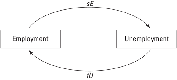
FIGURE 7-7: Flows in and out of employment.
 The interesting thing is, if in a certain month the flows from one state (employment or unemployment) to another are larger than the flows in the opposite direction, this impacts the flows in the following month. Eventually the flows in and out of employment (or unemployment) become equal.
For example, imagine starting in a situation with 400 unemployed and 1,800 employed. The rate of job finding is 0.625, and the rate of job separation is 0.05:
- In the first month, 250 unemployed people find a job, while 90 employed people lose theirs. As a result, employment grows by 160 to 1960 while unemployment falls by 160 to 240.
- In the second month, 150 unemployed people find a job while 98 employed people lose out. This leaves 188 unemployed and 2,012 employed.
This process continues. Notice that the number of unemployed people who find a job is falling every month and the number of employed people who lose their job is increasing every month. This is because the total stock of unemployed people is falling and the total stock of employed people is rising. In equilibrium, the number of people finding work is exactly equal to the number who lose their job:
In our example, this happens (approximately) when U = 163 and E = 2,037, and the unemployment rate of 163/2,200 ≈ 0.074 or 7.4 percent. You can use the above equation along with the fact that L = E + U to solve for this rate algebraically by substituting L + U for E to get the following equation:
With s = 0.05 and f = 0.625, this equation says the natural rate is again 7.4 percent. More generally, it shows that whether the labor force is constant as in our example or growing as in the true long run, the natural rate depends only on the rate of job separation (s) and the rate of job finding (f). Anything that raises (lowers) s or lowers (raises) f will raise (lower) the natural rate.
Thinking about policies to reduce the natural rate
Trying to tame the business cycle — trying to keep cyclical unemployment to a minimum — is a central task of monetary and fiscal policies or macroeconomic policy more generally. The frictional and structural problems that lead to a positive natural rate though are largely microeconomic. So, the best policies to lower it are microeconomic ones that go to the root of the problems.
Sometimes such micro policies are called supply-side policies because unlike the macroeconomic choices of monetary and fiscal policies, they don’t work by changing the overall demand for goods and services. Instead, they target micro aspects of the labor market that make it function inefficiently and that lower the productive capability of the economy. Applied to the labor market, such microeconomic policies attempt to reduce the rate of job separation (s) and increase the rate of job finding (f).
Here are some microeconomic policies that may help reduce the natural rate:
- Make sure jobs are widely advertised to the unemployed, for example, use online sites and job centers to speed up the rate of job finding.
- Ensure that unemployment benefits aren’t so generous that they discourage workers from exerting effort in their job search. Overly generous unemployment benefits can increase unemployment because they reduce the incentive to look for work. But they need to be generous enough that workers take the time to make “good” matches — ones that won’t quickly lead to new separations and more searching.
- Ensure labor market flexibility. Perhaps surprisingly, making it very difficult to fire workers can increase the natural rate. How? If firms know that firing an unproductive worker is difficult, they become reluctant to hire in the first place. This can reduce the rate of job finding and raise the natural rate.
There are many other micro-based policies to reduce the natural rate of unemployment. They’re not always easy to implement, and their impact may not be large. But in places like Spain and Italy, where the natural rate of unemployment is 10 percent or higher, even small reductions are helpful.
Quantifying the costs of unemployment
Macroeconomists study the costs of unemployment for a number of reasons. First, policies to reduce unemployment are only efficient if they impose less cost than the unemployment they eliminate. If reducing the unemployment rate by 1 percent would cut unemployment costs by $50 billion each year but requires a program with an annual cost of $75 billion, it’s not worth it. Better just to spend $50 billion to directly compensate those who bear the costs (which by the way is pretty much what unemployment compensation does). Second, and relatedly, it’s important to know who does incur the costs of unemployment. Is it only the unemployed themselves? Or are there external costs that fall on others?
Costing unemployment at the individual level
So what do we know about the costs of unemployment? Well, we know that the costs are high for those who suffer either a long unemployment spell or who are frequently unemployed for short spells. On average, the unemployed have worse mental and physical health, experience higher divorce and suicide rates, and report lower levels of life satisfaction.
Further, there are additional costs borne not by the individual workers, but by their families and communities. Children of an unemployed parent have worse health outcomes and perform worse in school. This can have repercussions that last a lifetime. The unemployed also participate less in school, church, and other community activities. Both violent crimes and property crimes are also associated with unemployment.
In short, the private and social costs of unemployment are significant. Programs like unemployment compensation that help individuals address some of these costs and social programs such as job counseling and retraining subsidies are likely worthwhile. Many of these policies are similar to those mentioned earlier. They improve matching or address structural issues and thereby lower the natural rate of unemployment.
Computing the costs of cyclical unemployment
As noted earlier, policies aimed at specific inefficiencies in the labor market have a microeconomic flavor. They work by changing the incentives of individuals and firms to promote a more efficient labor market equilibrium.
Policies that address cyclical unemployment aim at moderating the business cycle itself and so are more purely macroeconomic in nature. However, as pointed out in Chapter 3, using monetary and fiscal policies to address cyclical unemployment has important costs. Easier monetary policy may pave the way to more inflation. Short-run fiscal deficits can lead to sizeable amounts of long-run debt. In general, efforts to address short-run problems like cyclical unemployment can undermine the credibility of government commitments to sensible long-run outcomes. Is the reduction of cyclical unemployment worth these potential costs?
Living by the (Okun’s) Law
Over 50 years ago, Arthur Okun, a macroeconomic policy-maker in the Kennedy-Johnson administration, discovered an important empirical relationship between unemployment and real GDP growth. His result has ever since been called Okun’s Law. It’s not a law like gravity or the speed of light. It’s a statistical relationship that can change over time. For the U.S. currently, Okun’s Law can be written like this:
Here, gGDP is actual GDP growth, and gTrend is trend growth, that is, the growth in potential. In other words, if we grow at the trend rate, unemployment doesn’t change. But a one-point rise in the unemployment rate from one year to the next means real GDP growth fell by 2 percentage points. To put it a bit differently, for every 1 percent rise in unemployment above the natural rate, the economy loses 2 percent of real GDP.
For example, in 2009–2010, the U.S. economy was in the worst phase of the recent Great Recession. Unemployment averaged a bit over 3.25 percent above the natural rate in each year. Accordingly, the U.S. real GDP should have been about 6.5 percent below potential in each year for a cumulative loss of 13 percent. Estimates by the Congressional Budget Office (CBO) suggest the cumulative loss was around 12.5 percent. It’s not a perfect fit, you see, but it’s close and it gets closer over longer intervals of time.
The fundamental import of Okun’s Law is that U.S. unemployment is very costly. In 2009-10, 12 percent of GDP amounted to $1.9 trillion of lost production. That’s an enormous amount that far exceeds just the production of those directly unemployed. It’s true waste in that we let resources stand idle and we can never go back and undo that loss. Unless the disadvantages of using monetary and fiscal policies to fight the recession are extremely high, that kind of loss makes such policies worth pursuing under any cost-benefit analysis.
Considering hysteresis
We’ve so far treated cyclical unemployment as largely distinct from frictional and structural unemployment. But it’s not. Matching problems often get worse during a recession. So do structural issues. For example, there is considerable evidence that the longer you’re unemployed, the less likely you are to get reemployed at a good job. Long-term unemployment leads to a loss of skills and perhaps good work habits. It reduces a worker’s marketability.
Some of these changes can be permanent. That is, the cyclical unemployment of a short-run recession may have long-run effects because it raises the natural rate. This is called hysteresis. It means that short-run departures from the long-run equilibrium can change that equilibrium itself. If high cyclical unemployment also raises the natural rate, it then means not just a temporary but permanent reduction in GDP. Of course, this raises the macroeconomic costs of cyclical unemployment further.
Cyclical unemployment is a rise in unemployment above the natural rate due to a recession. Okun’s Law indicates that this has large macro costs. Every 1 percentage point rise in the unemployment rate above the natural rate pushes real GDP 2 percentage points below potential. Also, there is the possibility of unemployment hysteresis such that serious cyclical unemployment can have long-run labor market effects by raising the natural rate. This raises the already large costs of cyclical unemployment.