Losing your faith: Confidence in the economy

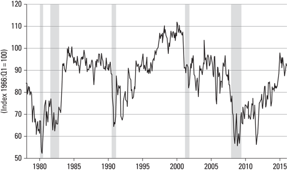
In life, confidence matters. Confidence can help you feel relaxed and perform better whether it’s a job interview or a first date. To an important extent, the same is true for consumers and businesspeople. They act differently when they feel confident about their economic future. For instance, the extent of consumer confidence can affect consumer spending. That’s the major reason that both the private business research group the Conference Board and the University of Michigan’s Institute for Social Research each report a (different) index of consumer confidence. The two move together fairly closely. Changes in either index can signal an upcoming change in households’ consumption decisions.

Figure 12-2 shows the Michigan Index of Consumer Sentiment from the beginning of 1978 to January 2016. Notice the steep slide from January 2008, when the index stood at nearly 100, to its recent bottom in late November 2008, when the index was approximately 55. That drop is undoubtedly connected to the onset of the financial crisis and the subsequent emergence of the Great Recession.

The long-run growth path is the economy’s anchor. While real GDP can wander off that path — occasionally above it, more often below it — the “invisible hand” that Adam Smith somehow saw (think about that when you have the time) is always there guiding real GDP Y back toward potential Y*. Thus, there are always forces pushing the economy back to its long-run trajectory.

This suggests that there is some normal or natural level of confidence as well. In other words, any measure of confidence has to be a relative one — evaluated relative to some norm. That’s what the Michigan and Conference Board measures do. They each survey a large number of consumers about both their personal finances and their expectations for the economy. Based on the number of positive versus negative responses to these questions, they then create a score that is normalized to be 100 in some base year (1966 for the Michigan survey and 1985 for the Conference Board one). The index in any other year will therefore give a measure of how upbeat consumers are feeling relative to a “normal” or base year. A confidence measure near 100 suggests that consumers are feeling their usual (long-run) confidence.

In other words, along the growth path, when consumers are thinking and acting normally, their confidence level will likely also be normal (we could even say natural). It will therefore be measured as 100 by either the Michigan or Conference Board measures. That’s why the Michigan index value of 100 before the financial crisis makes sense. The years leading up to the crisis had been reasonably good, and consumers were feeling reasonably confident.

Events like the financial meltdown can, of course, undermine consumer confidence. However, that confidence can change for non-economic reasons, as well. An outbreak of war, or possibly bad news on oil prices, or maybe climate change can be the catalyst for such shocks. This was a central element in the work of John Maynard Keynes. Much as economists like to use rational models to describe human behavior, Keynes felt that, in the aggregate, society’s behavior often reflected what he called animal spirits. Sometimes people are just more confident about the future than at other times, and it doesn’t have to be for any discernible reason. Keynes felt that this kind of irrationality was especially common among businesspeople. But it was clearly important for consumers, too.

Falling back in the short run

Suppose then that starting from a point with the economy at its full-employment potential Y = Y*, consumer confidence falls from 100 to, say, 90. What will be the impact on the economy?

The fall in confidence means that households are more worried about the future. This leads them to save more so that they’ll have a little something to fall back on should their fears materialize. Of course, the flip side of savings is consumption. The sudden rise in the savings rate also means a sudden drop in C. Remember, though, that C is a component of aggregate demand: AD = C + I + G + NX. So, aggregate demand falls too. At any given price level, fewer goods and services are demanded. We represent this in Figure 12-3 by a shift in the AD curve from AD₁ to AD₂.

As we discuss in Chapter 11, prices are sticky in the short run. Consequently, the inward shift of the AD curve causes the economy to move along the short-run aggregate supply (SRAS₁) curve from point A to point B. Prices do fall a bit, but the bulk of the adjustment falls on real GDP. Firms respond to the lower demand by cutting output and hiring less labor — shorter hours if not fewer workers. Output drops below potential or natural GDP from Y* to Y₂, and the unemployment rate rises above the natural rate. In short, there is a recession.

Returning to the long run

As we’ve stressed many times, the long-run path is the economy’s natural resting place. Sooner or later, the economy will return to its potential Y*. From the situation in Figure 12-3, there are two ways this can happen. One is that the fall in consumer confidence is temporary. Once Y stops falling, at Y₂ in Figure 12-3, consumers may feel that the worst is over or just become more upbeat for other reasons. This will reverse the process. The savings rate will fall, consumption and therefore aggregate demand will rise, and the AD curve will shift back to AD₁ so that full-employment output Y* is restored. This may in fact be the most likely scenario.

The other possibility is that while confidence gradually returns to normal, the experience of the economic downturn or other news is so disturbing that households permanently raise their savings rate. In this case, the path back to Y* is different. Instead of a reversal of the initial shift in the AD curve, the adjustment now comes from aggregate supply, as shown in Figure 12-4. Remember, wages and prices are flexible in the long run. The extra unemployment at Y₂ leads workers and firms to lower their wages and prices, respectively. As a result, the AS curve shifts down from AS₁ to AS₂. The economy now moves along AD₂ until real GDP reaches potential at , higher than the initial potential output . Unemployment returns to the natural rate as well. Why has Y* increased? Because society has adopted a permanently higher savings rate.

The short-run recession that resulted from the rise in the savings rate from s₁ to s₂ might initially lead you to think that increased savings is a bad thing. Certainly, it can be harmful in the short run. However, there is no paradox of thrift in the long run. If the savings rate permanently increases from s₁ to s₂, total savings permanently rises from s₁to s₂. In turn, this means a permanent rise in capital formation and therefore in the amount of capital each generation of worker has available. It will therefore lift the long-run path so that Y* will now be higher in every period. This can mean greater living standards for all in the long run.

So, yes, a temporary rise in the savings rate can hurt the economy, but if it becomes a permanent rise it can eventually help. Whether the permanent rise is good or bad in the long run depends on whether the initial savings rate s₁ was below or above the golden rule savings rate (described in Chapter 8). Most economies are well below the golden rule rate, so raising the savings rate likely helps in the long run.

Feeling confident enough to invest?

Decisions about how much to consume today and how much to save tomorrow obviously depend on how confident a household is about the future. If they get it wrong — if, for instance, they save a little more today than seems warranted — looking back later, they can undo that extra savings with relative ease. They just need to consume a little extra now and they’ll be back on track for their retirement or however far their planning horizon extends.

It’s different for firms. If a firm builds a new plant or adds to an existing one, or even if it buys a lot of inventory to support its new production line, it may have to live with the consequences for a long time. New plant or new equipment tends to be specialized or tied to the firm’s specific product line. If the firm finds that this capital is not profitable, it may not be able to sell it off very easily. Likewise, if a new product turns out to be a dud, it’s going to be hard to sell off the inventory of that product except at a significant loss.

Remember, the firm’s desired capital stock (see Chapters 6 and 8) is determined by the marginal productivity condition:

But if you’re going to have to hold the capital for many periods, you’ll want capital’s marginal product MP_K to cover the real interest rate and depreciation cost for each of those periods, too. That means businesses have to make a prediction of the marginal cash flow a new capital investment will make for a number of periods into the future.

That kind of prediction is fraught with uncertainty. Even a small change in the anticipated business climate may make an investment that once looked profitable now seem unattractive. And changes in the political environment, such as expectations of tax policy, can change the calculus of capital investment, too. Note that we’ve been talking in terms of anticipations and expectations. For business capital investments in particular, what’s important is not so much the cash flow that the project will generate right now, but the typical cash flow that it’s expected to generate in each of the many periods to come.

As noted earlier, Keynes felt that the expectations businesspeople held for future profitability were quite variable — possibly in an irrational way. That of course is exactly the meaning that the term animal spirits is meant to convey. In his view, business confidence or optimism is likely to be even more unstable than consumer confidence. For evidence, Keynes (and others) simply noted the empirical fact that investment spending bounces around a good bit more than does consumer spending.

Overall, the short run effects of a decline in business confidence are qualitatively much the same as a decline in consumer confidence. Feeling less optimistic about the future, businesses cut down on their investment spending for new capital I. Hence, aggregate demand falls as well, since AD = C + I + G + NX. In the short run, price stickiness means that the decline in demand leads to a fall in real GDP, so that Y falls below Y*, and unemployment rises above the natural rate, just as in Figure 12-3.

In the long run, though, the economy will again adjust. Output will return to its potential level Y*, and full-employment will be restored. If the initial savings rate is maintained, the long-run path will be unaffected by this short-run shock. But if the initial shock leads to a permanent rise in the savings rate, the economy will eventually begin to equip each generation of workers with more capital. The long-run growth path and with it Y* will shift up.

Fulfilling expectations and multiplying equilibria

There are a number of points that are important to make about the kind of exogenous shocks to consumer and business confidence that we have been describing. First, confidence levels react to the economy as well as act upon it. Households and consumers feel less upbeat in a downturn than they do in a boom. So, we can’t really claim that consumer and business confidence are totally exogenous.

At the same time, though, it’s clear that “out of the blue” shocks like those in the examples above also happen. For instance, on October 19, 1987, the U.S. stock market fell 22 percent without any real warning and without any sudden revelations of impending economic disaster. There was no report of a collapse in corporate earning or any news of a sudden war or other political upheaval. It was clearly just a case of investors in the U.S. and around the world suddenly losing faith in the economy. It was a truly exogenous event.

Second, it’s the large shocks that we worry about. Small day-to-day gyrations in consumer and business confidence are inevitable. Thankfully, these don’t have much effect. It’s the larger shocks to confidence and to aggregate spending that cause problems.

Third, while the economy eventually gets back to full employment in all cases, that typically takes a long time. Once the economy starts to decline, it usually takes a year and a half or longer to recover fully. And sometimes the process can be very long. It was nearly 12 years before the economy was back on its feet after the crash of 1929. In 2016, the U.S. economy is only just approaching its long-run growth path after sliding into recession in late 2007. During all that time there is a waste of unemployed or underemployed resources and lost production opportunity.

Finally, and perhaps most interestingly, declines in consumer and business confidence can be self-fulfilling. Consumers and/or business leaders begin to worry that the economy is not healthy and, as a result, cut back on their consumption and investment spending. Because prices are sticky, this decline in spending in fact leads to the very economic slowdown and weak business conditions that everyone feared.

This is really a way of saying that the economy may have more than one short-run equilibrium. One comes about when everyone expects full employment and therefore spends at a level that keeps the economy actually at full employment. Another equilibrium can occur, however, in which consumers and business leaders fear a recession and therefore cut spending to levels that make a recession happen.

Economists now know a fair bit about settings with multiple equilibria. Sometimes it doesn’t really matter which equilibrium is selected. For example, everyone driving on the right-hand side of the road or all on the left-hand side is each an equilibrium and there’s little that favors one over the other. The existence of more than one equilibrium in that case is not so worrisome. In some cases, though, and the short-run macroeconomy is one of them, the equilibria can be ranked. Everyone acting with confidence to produce a healthy, fully employed economy is a lot better than everyone acting doubtfully to produce the weak economy that confirms those doubts.

What economists know about multiple equilibria settings is that the outcome can be fairly fragile. In the absence of a central, coordinating device — for example, double yellow lines and a legal authority that says you need to stay on the appropriate side of the road — the equilibrium can easily move, and there is no guarantee that the outcome will be the good one. In other words, Adam Smith’s “invisible hand” is not enough to guarantee a happy economic ending. In the short run — which, remember, can last a while — it might guide us to the “wrong” equilibrium with low output and unemployment above the natural rate.

Impacting demand via fiscal policy

Fiscal policy refers to government budgetary decisions. Ultimately, it has two parts:

• How much to spend on various activities and programs
• How to finance those expenditures

Here the choice is (mainly) whether to fund current expenditures with tax revenues or to borrow. Thus, fiscal policy also includes issues of debt management.

The funds borrowed to finance government expenditures are drawn from the funds households have left after consuming and paying all their taxes. Basically then, government borrowing is funded by private sector savings. Because it diverts those savings away from capital formation (generally), fiscal policy impacts the national savings rate and capital formation.

Yet fiscal policy also impacts aggregate demand. Specifically, changes in fiscal policy also shift the aggregate demand curve in the AD–AS model. We discuss fiscal policy in detail in Chapter 15, but here we offer a quick preview of fiscal policy in the AD–AS model.

Expansionary and contractionary fiscal policy

Expansionary fiscal policy is a rise in government expenditure or a cut in taxation. Either of these policy changes affects the economy by increasing aggregate demand. Contractionary fiscal policy is a decrease in government spending or an increase in taxes. It shifts the AD curve in.

Government expenditure G is a component of aggregate demand: AD = C + I + G + NX. It is for the most part an exogenous component in that how much we spend on public goods and services is the result of a political process. That is, spending is largely determined by a budget set by Congress or other (state or local) legislative body. As a result, it’s easy to run thought experiments about what happens when authorities decide to increase G. And the answer is that it’s qualitatively the same as when consumer or business confidence rise. A rise in G will shift the AD curve outward just like a rise in consumer or business confidence that would raise C or I, respectively.

Tax changes are slightly, but only slightly, different. One difference is that tax changes or, more usually changes in tax rates, are not components of aggregate demand themselves. Instead they work indirectly to influence components of aggregate demand. The other major difference is that tax changes work in the opposite direction of government spending. Thus, while an increase in G is expansionary and will shift the AD curve outward, it will take a decrease in taxes to have this effect. Tax cuts do this by inducing:

• Increased consumption C: Consumption is highly influenced by the amount of disposable or after-tax income people have. This is given by (Y – T), or gross income less tax liabilities. Often we can represent tax liabilities with a linear function such as T = –T₀ + tY. Here, T₀ is the safety net payment you receive if your gross income is 0 (so it’s a negative value), and t is what economists call the marginal tax rate — the fraction of each additional dollar that gets taken away by taxes. So, if T₀ were $5,0000 and t = 0.2, you would receive $5,000 if you had no other income but only keep 80 cents of each dollar that you earned after that. Disposable income is: Y – T = Y – (–T₀ + tY) = T₀ + (1 – t)Y. Cutting taxes amounts either to increasing T₀ or decreasing t. Either one increases disposable income. When people have more disposable income, they consume more.
• Increased investment I: If the return on capital investments is taxed at some rate τ_C, then firms don’t get to keep all the profit on their capital investments. Formally, our condition for firms being at the capital stock they want (see Chapters 6 and 8) now becomes this:

  

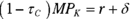
  Thus, as the tax τ_C falls, the net or after-tax marginal product that makes the condition hold falls, too. This means that the amount of capital firms want rises since capital is subject to diminishing marginal returns. Basically, lower taxes mean that firms get to keep more of the profit that capital generates. In turn, this makes firms want more capital and that boosts current investment.

As noted, expansionary fiscal policy will shift the AD curve out, whether it is due to an increase in G or a fall in T (or both). The short-run impact on the economy is to raise AD. Thus in Figure 12-5, aggregate demand has increased from AD₁ to AD₂, which in the short run causes output and the price level to rise. You can see this as a movement from point A to point B — because prices are sticky in the short run, the price level hasn’t risen by much. As time passes and prices become more flexible, short-run aggregate supply (SRAS) shifts up and to the left, raising the price level and reducing output until eventually output is unchanged at point C.

In short, expansionary fiscal policy gives the economy a short-term boost and raises incomes and reduces unemployment. But this boost is short-lived. After prices adjust, output returns to its natural level, and unemployment returns to its natural rate. Contractionary fiscal policy would, of course, work in reverse — reduce GDP in the short run but leave it unchanged in the long run.

Changing demand via monetary policy

Monetary policy reflects the choices made by the Fed (or the central bank in other countries) regarding the money supply, with a view to influencing the economy. (For a detailed look at monetary policy, check out Chapter 14.) As with fiscal policy, these choices are made outside the model and so are exogenous, though of course they may respond to macroeconomic developments. The important thing again is that monetary policy shifts can also shift the AD curve. A policy that shifts the AD curve out or to the right is expansionary. One that shifts it in or to the left is contractionary. Once the AD curve shifts, the price level, real GDP, and unemployment will all change as we move along the aggregate supply curve.

Monopoly money

Someday, somewhere, someone may well ask you, “How much money do you make?” If so, what should your answer be?

You might say, “None of your business.” Or decline to answer more politely. Or, if you are feeling unusually obnoxious, you might report a six- or seven-figure salary and add, “So there!” However, there is in fact a very precise and (hopefully) correct answer that you can always give, namely, “zero.” The fact is, you don’t “make money.” What you legally make is part of GDP and what you earn is income. Only the Federal Reserve, in cooperation with the Treasury, can “make” money. Anyone else who does it is engaged in counterfeiting, and you can go to jail for that. So don’t ever say any positive amount when asked, “How much money do you make?” You never know if you’re talking with an undercover law enforcement official.

That’s why the Fed or any central bank is such a powerful institution. It has a monopoly over the creation of money. It controls the supply of money assets that the economy can use for liquidity purposes. Like any monopolist, that control of supply gives the Fed control over the price or opportunity cost of money … and that’s the nominal interest rate as we’ve just seen.

Figure 12-6 illustrates the money market. The downward-sloping demand curve reflects the fact that as the nominal interest rate rises, so does the opportunity cost of holding money, and therefore there is less demand for it (again, all else equal). The two vertical supply curves show different choices for the given supply of money that the Fed chooses. If it chooses to keep the money supply low at M₁, the nominal interest rate will be high at i₁. But if it chooses to set the money supply at a higher amount M₂, the nominal interest rate will fall to i₂.

Thus, the Fed can use its control of the money supply to set the nominal interest rate. In fact, the process typically works in reverse. The usual case is that the Fed announces the interest rate that it wants, for example either i₁ or i₂, and then supplies the amount of money (M₁ or M₂) to hit that interest rate target. Because the demand for money and other economic conditions isn’t perfectly predictable, the Fed usually sets a range for the target rather than a single precise value.

For example, from December 2008 until December 2015, the target range was an ultra low 0 to 0.25 percent. At the end of 2015, however, the Fed very slightly raised the target range to 0.25 to 0.5 percent. Of course, that range does not refer to the interest rates you and I pay. It instead refers to the interest rates paid on so-called federal funds — the cash banks lend to each other on a very short-term basis. But as Chapter 1 points out, the financial markets are tightly integrated. As the Fed raises the federal funds rate, interest rates in other markets rise as well.

Expansionary and contractionary monetary policy

In order to carry out an expansionary monetary policy, the central bank would choose the money supply to reduce the interest rate in the money market. Returning to Figure 12-6, the central bank will select a high money supply such as M₂ to push the nominal interest rate to the lower value i₂. As noted, this will push the real interest rate down as well. That’s critical because that’s what determines people’s spending. Here’s how it works.

• Increased consumption C: Reduced real interest rates make borrowing cheaper and saving less attractive. Households raise their consumer spending, especially on big-ticket items such as cars and major appliances.
• Increased investment I: Perhaps even more important than the consumer spending effects is the fact that the fall in the real interest rate raises the desired capital stock. So, firms invest in more capital.
• Increased net exports NX: When the Fed decreases interest rates, U.S. investors can do two things. They can (and will) move out of U.S. bonds and into holding more dollars because the opportunity cost of doing so has fallen. But they can also take funds out of U.S. bonds and put them into foreign ones. If domestic and foreign bonds were previously paying the same interest rate, foreign bonds now look more attractive. So, when the Fed increases the money supply, not only will people hold more domestic money balances, they’ll also try to buy some now higher-yielding foreign assets. To buy foreign assets, though, they have to buy foreign exchange. The extra demand for foreign assets (and the decreased demand for U.S. assets) will therefore translate into a now higher demand for foreign money and less international demand for U.S. dollars. As a result, the dollar will depreciate and this will turn into a real depreciation given price stickiness. (Check out the section “Purchasing Power Parity” in Chapter 9). U.S. goods therefore become cheap relative to foreign goods. Consequently, U.S. and foreign residents both find U.S. goods more attractive and foreign goods less attractive. This in turn leads to a rise in net exports NX.

By now, you’ve internalized the fact that consumption, investment, and net exports are each an element of aggregate demand (AD = C + I + G + NX). So, expansionary monetary policy boosts AD. You can model the effect on the economy using the AD–AS model (see Figure 12-7).

In a similar way to expansionary fiscal policy, then, expansionary monetary policy has boosted aggregate demand from AD₁ to AD₂. In the short run, this causes output and the price level to rise (a movement from point A to point B in Figure 12-7). Sticky prices in the short run mean that the price level doesn’t rise by much at first. In the long run, prices become more flexible, and the SRAS curve shifts up and to the left, raising the price level and reducing output until eventually output is unchanged.

It shouldn’t take much to convince you that contractionary monetary policy just runs the foregoing scenario in reverse. In this case, the Fed reduces the money supply from M₂ to M₁ and thereby raises the nominal rate to i₁. In the short run, this turns into a real rate increase that directly induces a fall in consumption C and investment I. It also indirectly induces a fall in net exports NX by leading to a real exchange rate appreciation. All of these developments imply a downward shift in the AD curve. Output will fall and unemployment will rise in the short run. In the longer run, though, as prices more fully adjust, the economy will return to full employment and real GDP will again achieve its potential Y*.

Noting the multiplier effect

All spending shocks, whether generated by a change in consumer and business confidence, fiscal or monetary policy, or other factors have a bigger impact on the economy than you may think. For instance, a drop in business confidence that leads firms to cut investment spending by $200 billion may well reduce aggregate demand and real GDP by $350–$400 billion. Why?

The answer lies in something called the multiplier effect. Remember that consumption itself is a function of disposable income, C(Y – T). If, to continue our example, business confidence declines and investment spending falls by $200 billion, AD and income will straightaway fall by the same amount. But that’s just the start of the story. Because as Y falls, so does disposable income. But because consumer spending depends on disposable income, it will fall again. Of course, this decreases real GDP and income still further.

Suppose that the $200 billion investment decline reflects a cut in new factory construction. Then the initial $200 billion drop in production also implies a $200 billion drop in the income of construction firms and workers. As a result, they cut their spending on, say, household goods and services such as entertainment, clothing, and so on. Imagine that this reduction amounts to half of the drop of the initial $200 billion fall, or about $100 billion. That’s another $100 billion of income that now those in the entertainment and clothing industries don’t have. Hence, they cut their expenditures as well. Again, let’s say this reduction is half of the fall in Y, or another $50 billion decrease. As this process spreads, the cumulative drop in aggregate demand and real GDP (in billions) is:

This is called a geometric series and there’s an easy formula to get where it all ends up. Let b be the fraction by which spending falls each round. In our example, b = 0.5. Then the total, cumulative spending effect is the initial shock divided by 1 – b. In our case, the initial shock is $200 billion and b is 0.5. So, the total change in spending is: $200 / (1 – 0.5 ) = $400.

As you can see, the initial shock induces several additional rounds of spending changes, with each smaller than the previous one and asymptotically approaching zero. Yet although they eventually fade to zero, the sum of all these additional effects greatly magnifies (economists say multiplies) the initial shock. In the example at hand, that original shock of $200 million was multiplied into a total shock of $400 million.

In this case, economists say that the multiplier is 2, because that’s the factor of increase over the original shock. Estimates of the multiplier vary. They depend on whether the initial shock is to spending or to taxes or to some private sector element like consumption or investment spending. The estimates also depend on whether the economy is at full employment or not, and what sort of exchange rate policy it has.

Note that so long as the short-run supply curve is not entirely flat, there is a difference between how much the shock shifts the aggregate demand curve and how much real GDP actually changes. Figure 12-8 illustrates this point. The initial shock to government spending was ΔG. This shifted the AD curve to the right by μ₁ΔG. So, μ₁ is the multiplier in terms of the effect of the shock on aggregate demand. However, because prices rose from P₁ to P₂, real GDP rose only by ΔY = μ₂ΔG. That smaller multiplier μ₂ is the one we can measure. Ultimately, it may be the one that’s more relevant because it incorporates the supply response. But it is a different measure than the spending shock’s impact on aggregate demand alone.

Conventional estimates of the multiplier for government spending G are based on analysis that implicitly incorporates some short-run price rigidity typically yields multiplier estimates ranging from 0.5 to 2, with 1.25 not a bad guess. Again, though, these are not estimates of how far the AD curve shifts but of the ultimate change in real GDP.

Running dry … or on empty

Imagine the economy running smoothly on its long-run growth path. To make things easy, imagine that it’s an agriculture-based economy producing mainly cotton, rice, and wheat. Suddenly, drought strikes — prolonged and severe. Without water, there’s no need for workers who would plant crops or to tend to them. There’s also no need for plowing and reaping equipment. So, as the drought wears on, men and machines stand idle. Unemployment builds.

But the problem is not that the economy is producing less than potential. It’s that the drought has suddenly reduced that potential itself. At least for the present, Y* has fallen. Figure 12-9 illustrates this case. The economy has moved from an initial equilibrium at point A with real GDP equal to potential GDP to a new equilibrium at point B with real GDP now equal to the lower value of potential given by . The economy is at full employment but it might not feel that way because fewer people are working at the lower level of potential output.

Assuming that the drought does not reflect permanent climate change, the process just described will be reversed once normal weather returns. But it may take a while to restore the economy to its long-run path.

The dramatic energy price increases of the 1970s are often regarded as a supply shock similar to a drought. Instead of shortfall of rain, though, it was a shortfall of oil and natural gas. But for a modern economy, energy supply is a lot like rain is for an agricultural one. Some inefficient capital equipment that is usable when energy is cheap simply is not worth using when energy is suddenly very expensive. The machines and the men that operate them become unemployed, and this can spread through the economy via multiplier effects.

Unlike the drought, the sudden shortage of oil and natural gas may be the start of an era of persistently high energy prices that reduce potential GDP both now and into the indefinite future. While the economy would, as always, return to its long-run path, that path will have shifted downward. The short-run pain of unemployment and output below potential will be over, but the loss from lower potential GDP is permanent. If this is the case, then the ultimate cost to the economy from this negative supply shock is larger than from any demand shock, which is always temporary in nature. Fortunately, painful as they were, the energy shocks of the 1970s do not appear to have been permanent. Adjusted for inflation, the price per barrel of oil today is not much higher than it was in 1976.

Supply shocks are important because they are not always easy to separate from demand shocks. Looking back over the past century of data, it now seems clear that at least some of the short-term movement in real GDP has been due to supply-sided changes in potential rather than demand-driven movements in output away from potential.

Indeed, part of the 1930s disaster (but not the whole story by any means) was in fact a horrible drought that cut through the entire Midwest from Minnesota to Oklahoma. Coupled with the fact that farmers in those days had poor soil and water management, the land literally dried up, giving rise to horrible dust storms and the nickname the Dust Bowl for much of the region. It was not a lack of demand that led to the migration of “Okies” and others. It was the impossibility of producing any supply.

Unfortunately, policy-makers will not always know at the time whether it’s a demand shock or a supply shock that’s driving the economy. So, designing the right policy response is difficult.