
Chapter 3
The Short Run and the Long Run
IN THIS CHAPTER
Understanding actual and potential GDP
Examining the short-run long-run distinction
Recognizing the benefits of a unified model
Considering long-run policy commitments and short-run policy flexibility
A modern economy produces and distributes a vast array of goods and services: cars, appliances, education, health services, sports equipment, and much more. In many if not most economies, the bulk of this activity is organized through a market mechanism, which is surprising really because you can’t see it or touch it.
As Adam Smith noted over 200 years ago, the market works like “an invisible hand” to guide a multitude of economic endeavors that result in consumers getting the goods they want at a reasonably low cost. For example, no one is directing all the people involved in getting bread to consumers (the flour producer, the baker, the delivery driver, the shopkeeper, and so on). No one needs to tell them what to make or when and where to trade — they just do it. Each producer is trying to do the best for herself, of course. Yet amazingly, their efforts end up doing well for everyone — all the bread-lovers get the fresh, tasty loaves they want while all the farmers, millers, and bakers get paid. Contrast that with the command-and-control bread production of the old Soviet Union where bread shelves were empty half of the time.
Similarly, it’s a safe bet that very few individuals have the knowledge and ability to create many of the things we buy, from soap to laptops to legal services. Even making a single pencil from scratch would be difficult. Yet you can easily go into a shop and buy a pack (or order them online). Again, the market economy succeeds in coordinating the activities of many different individuals to a productive end.
So, economists love markets where individuals meet to trade for their mutual benefit and so many different goods and services are exchanged. But however much you love something, you have to admit that occasionally it can misfire. Even the most ardent Star Wars fan has to concede that The Phantom Menace was a mistake. Similarly, even economists realize that market economies can sometimes get sick. Fortunately, both movie franchises and the economy can also heal and recover.
In this chapter, you’ll learn about the economy’s health in the short run, when it can get sick, and in the long run, when it can recover from a temporary (if prolonged) illness and get back on its normally healthy track. You’ll also get a sense of the different approaches macroeconomists take when thinking about the short run and the long. The difference between these time frames also raises complications for policy-makers. Following surgery, a doctor may prescribe strong pain medication for a short period of time, but you don’t want this to become a long-term need. Similarly, the best practice for dealing with short-run difficulties may be very different from what makes for a good long-run macroeconomic policy.
Separating Trend and Cycle
A good physical examination typically includes a temperature, pulse, and blood pressure reading. Blood work to check cholesterol and glucose levels is also common. And if you’re lucky enough to have reached 50 or so and be male, you’re also likely to get your prostate probed. None of these procedures would be very informative, though, without some measure of what’s healthy or normal. And the standard of good health can change over time.
For example, in the U.S., a passenger car with a fuel mileage rating of 20 MPG would have been a standout in 1975, when the average across all cars was 13.5 MPG. But that 20 MPG rating today would look positively sick given that average MPG has since climbed to over 31. Likewise, in olden days, even a glimpse of stocking was enough to shock people. Now? Well, now the Vermont Teddy Bear Company will not only ship you a fuzzy stuffed bedtime companion but a collection of intimate toys from Fifty Shades of Grey to go with it.
Over time, the real GDP that’s consistent with a healthy economy changes too. For one thing, the workforce grows. So does the capital machinery available to them. On top of that, both the workers and the machines become more productive due to education and technical progress. So, what we’re capable of producing when operating at top form rises with each year. Economically speaking, 1965 may have been a good year for the U.S. But if we were still producing today the level of GDP that we produced then, we’d have to conclude that the last 50 years have not turned out very well. In short, we need an evolving standard of economic health if we are to identify at any point in time how well or how sick the economy is.
Rising potential GDP over time
As noted in Chapter 2, the U.S. real GDP has grown by about 2.8 percent on average each year since 1965. Where does that trend come from? Remember that GDP is production — that is, output. In turn, GDP can be expressed as the total labor force times the amount each worker produces [Q = L × (Q / L)]. It follows that underlying that trend, GDP growth is some combination of a) growth in the labor input, and b) growth in the productivity of that labor. As for the first of these, the labor force can change for a number of reasons. The main one of course is population growth. More people generally means more workers. Obviously, this relationship does not hold strictly at all times. Changes in the average age of the population or net immigration can also affect the growth of the labor force at a given time.
 Over the long run though, the labor force and the population overall grow at pretty much the same rate.
Output growth that emanates just from more input growth is not very sexy. That’s because it doesn’t indicate any increase in the general well-being or most people’s standard of living. For that to rise, we need to have gains in output per worker, or productivity growth. Fortunately, that tends to happen as well over time for two reasons. One is that businesses invest in new capital, and workers are more productive as they have more machines to work with. The other is technical progress — both workers and machines get smarter with each generation, though among people there are some notable individual exceptions, to be sure.
Over the last 50 years or so, the workforce has increased by a bit over 1 percent each year, while worker productivity has grown on average a bit less than 2 percent (though recently it seems to be slowing). Together, these two factors account for the roughly 2.8 percent growth in real GDP that the U.S. economy has averaged for some time. Because an aging population means a smaller fraction in the labor force, and as the economy turns from manufacturing to services, we may expect some further slowing down in the growth of potential GDP. The Congressional Budget Office (CBO) estimates that it has been more recently growing at 2.25 percent.
Cycling through the short run: Minding the gap
Whether the number is 2.8 or 2.25 percent, it is important to remember that it is just an average. In case you hadn’t noticed, the actual change in real GDP is often quite different from that average value. In some years, real GDP not only fails to grow at 2.8 percent but actually declines a fair bit, and so does employment. For example, real GDP fell by nearly 2 percent in 1982 and by over 3 percent in the first quarter of 2009. Those numbers may not seem very large, but a move from growing positively at close to 3 percent to declining at a rate of more than 3 percent implies an overall swing of about 6 percent. In 2009, the normal or trend rate of real GDP was over $15.5 trillion. So, the swing that year meant a loss of over $1 trillion of production — which would be a lot even in Canadian dollars.
Note that if the long-run average growth rate is 2.8 percent, then periods in which growth is below that level must be balanced by periods in which it is above it. A bust must ultimately lead to a boom and recovery, and vice versa. From this viewpoint, it’s sensible to categorize the average 2.8 percent growth path as the long-run trend, while the actual path that includes the significant falls from and rises back to that trend show the result of the business cycle. The natural question then is: What’s happening over the short-run cycle that is different from what’s driving the long-run trend?
In many ways, the long-run trend is a supply-side concept. It is a measure of the output the economy can produce given normal growth in the amount of labor supplied and normal productivity gains. Trying to produce more than that for very long would ultimately require digging much deeper into the population to find more willing and suitably skilled workers, along with getting more raw materials and other inputs. Even then, finding a place to put the extra workers could be difficult as plant capacities would be strained. Shortages would ensue, and inflation would start to rise. Similarly, producing less than the trend supply would leave excess capacity, redundant or unemployed workers, and downward price pressures. For this reason, the trend path is somewhat equivalently referred to as potential GDP. It designates, at any point of time, the level of GDP that the economy can produce without putting any extra demands that exceed normal growth but also without leaving any resources seriously unemployed.
Figure 3-1 graphs these two different measures of real GDP from 1990 through the third quarter of 2015, both taken from the Federal Reserve Bank of St. Louis. The straighter line is an estimate of trend or potential GDP. The more jagged line shows the path of real GDP as it actually has transpired, complete with the ups and downs of observed business cycles. The difference between the two — expressed as a percentage of potential — is known as the GDP gap. As already noted, the GDP gap was a little over 6 percent in early 2009. The U.S. economy was producing less than 94 percent of what it would have produced in the absence of the 2008 financial shocks.
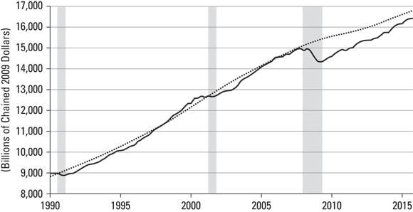
Image source: Federal Reserve Bank of St. Louis
FIGURE 3-1: Potential GDP is represented by the straighter (dotted) line, and actual GDP by the more jagged (solid) line.
Waiting for GDP: Why is the short run so long?
As Figure 3-1 suggests, and as the underlying data confirms, the GDP economy deviates from the potential trend with some frequency, usually in the downward direction. Busts or using the slightly more technical term, recessions, happen. From time to time, GDP falls (or grows very slowly), and the economy slips below potential, but eventually, the economy rebounds and returns to the trend.
Sometimes we even produce more than the potential GDP. The late 1990s is such a case. But such negative GDP gaps are rare, short lived, and small. That’s why the average GDP gap is a shortfall of roughly 2 percent. In the typical case, the recovery that follows the initial downturn takes a fair bit of time to bring the economy back to its trend path.
Thanks to the National Bureau of Economic Research (NBER), we can actually put some numbers to this. The NBER is not a government agency. It is a private, non-partisan research institute funded largely by corporate and foundation donations. Much of the NBER’s early work focused on business cycles, and, with time, it has become the nation’s quasi-official arbiter of recessions and recoveries. When an economist says that the recent U.S. Great Recession began in December 2007 and ended in June 2009, she is relying on dates identified by the NBER.
If you look again at Figure 3-1, you might wonder about this. Even in 2015, the economy is still producing 3 percent less than potential. How was the recession officially over in 2009?
The answer is that a recession refers to a fall in real GDP, not simply being below it. Once real GDP stops falling, the recession is over, and the recovery or expansion, which is a rise in GDP, begins. During this period, economic activity or GDP increases until it hits its next peak. That happens when the next recession begins and GDP starts falling again. The NBER business cycle-dating committee determines the precise dates of each — looking backward. No mortal, except maybe Leonard Cohen, can see the economic future.
Say a recession happens. GDP starts to fall as it did in late 2007 and continues to do so for some time, perhaps for 18 months into June of 2009, again as with the most recent case. All that time, potential GDP is growing. So, the gap is widening. Even if actual GDP begins to grow at a 2.8 percent clip in 2009, it will merely stop the gap from getting bigger. To close the gap, actual GDP has to rise faster than potential.
In the U.S., the average recession length in the eight downturns since 1960 is about 11 months. Fortunately, recoveries last a good bit longer—close to five-and-a-half years on average. The bad news is that actual GDP growth, though faster than trend, is still sufficiently slow that it takes about all of this time to get the economy back to producing its potential GDP.
Suppose for example that real and potential GDP are both $15 trillion at the end of 2007 but that by early 2009, the GDP we could potentially produce if we employed all those seeking work and utilized all our plant and equipment to capacity had grown to $15.41 trillion (about 2.2 percent growth annually). Meanwhile, owing to the recession, actual GDP has declined to $14.45 trillion. The GDP gap in early 2009 will then be 6.2 percent. Now suppose that potential GDP continues to rise at 2.2 percent (to be conservative) while a recovery begins in which actual GDP rises at 3 percent. If these relative growth rates continue, it will take about eight years for the economy to get back to potential.
That’s a long time — especially for those who lose their jobs, which is of course what happens in a recession. When fewer goods and services are being produced, firms no longer need as many workers as before. Unemployment rises. People want work but can’t find jobs. Some of those who do find work, though not unemployed, are still underemployed relative to their skill levels, as when former applications designers or business executives find themselves flipping burgers or driving for Uber. And it’s not just people either. Factories and plants are also underutilized and in some cases shut down. In short, a lot of productive resources go to waste, and a lot of valuable goods and services go unproduced.
The big question is why. Why do recessions happen? And why do recoveries take as long as they do to return the economy to its full potential? Why doesn’t the miracle of the “invisible hand” work to avoid the waste of a recession?
We’re going to talk a lot about these issues and what the government can do to improve matters in the chapters to come. We can preview the main forces here though. First and foremost, most recessions start with a drop in the amount of goods — consumer goods and new capital goods — that households and businesses want to buy. That is, most recessions start with a fall in aggregate demand.
Note that a fall in demand doesn’t have to lead to a fall in production. If workers take sufficiently deep wage cuts and firms make correspondingly large price cuts, the smaller amount of consumer and business spending will still buy a lot of output. This is in fact the automatic adjustment mechanism relied on by classical macroeconomists to keep the economy at its potential. For reasons not completely understood, though, this automatic adjustment doesn’t seem to be strong enough in the short run. Wage and price reductions, or at least slower rates of wage and price increases, do not happen easily. Instead, the fall in demand translates into a fall in GDP and employment. And it is only after that rise in unemployment that the needed wage and price reductions seem to happen. Unfortunately, even then these adjustments happen slowly enough that the time from initial downturn to a full recovery can be long.
It is also worth noting that sometimes the decline in GDP reflects a supply and not a demand shock. Think of an agricultural economy that produces just one good, say, sugar or tobacco. If there is a serious drought, production will fall; so will the employment of machines and workers. There is no reason to employ harvesting machinery and laborers if there is no crop to harvest. Output will be down, unemployment will be up, and we will have recessionary conditions. But it’s a supply-induced decline. No matter how much consumers and businesses want to spend, output cannot be increased. What it really amounts to is not a fall below potential GDP but a temporary (we hope) reduction in that potential output itself. The OPEC price shocks of the 1970s that made energy-intensive capital no longer useable may have had a similar effect.
For the most part, we focus on demand shocks. Those likely reflect the bulk of the unusual movements we observe in the path of actual GDP. They are also the kind of shocks that macroeconomic policies can best address.
Unifying the Field (or Not)
Economists often are accused of suffering from “physics envy.” (Except when it comes to academic salaries.) This is because economists want to develop theories that have the same widespread explanations of economic events that physics can provide for natural phenomena. To put it mildly, economics is a long way from that point.
But physics is not yet quite where it wants to be either. Notwithstanding the claims of some string theorists, physics is still looking for Einstein’s unified field theory that will put quantum mechanics and general relativity together in one grand “theory of everything.”
To some extent, macroeconomics has been plagued with the same problem. In particular, it has been bifurcated between a long-run analysis that can explain the features of the economy along its trend path, and models of the short-run that capture the disequilibria associated with recessions and unemployment. Like physicists, however, economists have recognized the attraction of building one model that is capable of explaining both the short run and the long in one unified theory.
Going both short and long in macroeconomics
As noted earlier, it is somewhat natural to envisage the potential or trend GDP path — based as it is on supply-side considerations — as reflecting the long-run equilibrium in which all variables can adjust to equate demand fully with that supply. Likewise, it is easy to think of recessions and slow recoveries as reflecting a short run in which various constraints make it impossible for consumers and businesses to make such adjustments. Excess supply — in particular, unemployed labor and capital — are the result. The question then is what are those constraints and where do they come from?
Because macroeconomics really came of age in the wake of the Great Depression — essentially a ten-year departure from trend in which real GDP was for a time more than a third below its potential and unemployment reached 25 percent — it is natural that much early macroeconomic analysis focused on the short run: How could the economy get into such a fix, and how could policy help it get out? This was certainly the perspective taken in John Maynard Keynes’s path-breaking volume The General Theory of Employment, Interest, and Money, the book that in many ways started macroeconomics as an important subdiscipline of economics overall.
In focusing on the short run, though, the underlying anchor of the long-run analysis was often left out. In other words, less attention was paid to making the short-run analysis consistent with the long-run model. A somewhat bifurcated approach to macro then emerged. For some purposes, economists focused on understanding the growth in potential GDP and what policies would best foster this growth. For other purposes, the focus was on behavior in the short run where disequilibrium might rule, especially a disequilibrium in the labor market with excess supply of (unemployed) workers.
As a practical matter, modeling the short-run as a disequilibrium meant developing relations (equations) that did not fully embody the rational, optimizing behavior that underlies the long-run model. Instead, it often meant deriving relations that captured the broad behavioral regularities of aggregate variables. For example, macroeconomists developed models of total household consumer spending or business investment spending based on simple historical relationships rather than trying to model the optimizing rational behavior of individuals in each group and then working out any equilibrium they might imply. The justification in part is that those aggregates result from the interactions of millions of individual agents, each of whom may be very different in terms of objectives and constraints. Trying to work out optimal behavior for each and put it all together to describe the macro economy is not possible. In some ways, it smacks more of microeconomics than macroeconomics.
The weakness of this approach is that, as physicists recognize, having two models can be a drag. In macro, it runs the risk that the story we tell about short-run analysis is inconsistent with the one we tell for the long run. To be sure, a fetish for consistency is the hobgoblin of small minds. But the problem is bigger than that. Policies adopted based on the short-run analysis may have very different effects in the long run. And model predictions of short-run outcomes may themselves go wrong if the model doesn’t allow consumers and businesses to optimize rationally over a reasonably long horizon. This is especially important with respect to expectations because rational agents are forward-looking. Their actions today reflect their expectations of what the future will bring. For example, we might think that a tax cut will lead consumers to spend more today. But it might not if those consumers anticipate that the government will later have to raise taxes to offset a current tax cut. In that case, they may just save today’s tax cut so as to have the money to pay those higher taxes down the line.
Generalizing equilibrium in a dynamic way
In recent years, an alternative macroeconomics approach has developed. It is generally referred to as the (deep breath) dynamic stochastic general equilibrium (DSGE) view. Here, the long- and the short-run outcomes are generated from a common model that emphasizes forward-looking agents who make rational choices to best achieve their objectives. In the absence of any shocks, these choices then lead to the trend or long-run path along which resources are fully employed, and real GDP achieves its potential.
Random (stochastic) short-run shocks lead to deviations from this path not because of any irrational or myopic behavior, but because of the more or less optimal rules agents choose for responding to shocks subject to the constraints they face. Often this is the result of recognizing market imperfections. For example, if it is common for firms to have market power, then firms have to have rules for setting prices. Likewise, imperfect competition in the labor market will lead to the adoption of rules for wage setting. In both cases these rules should be consistent with the long-run equilibrium so long as there are no shocks. At the same time, though, these same rules may lead to slow adjustment of wages and prices if there is a shock.
This more recent approach is thus more general in that it incorporates the long and the short run into a common framework. The DSGE approach is also more logically consistent in that its predictions are rooted in rationality. Again, this is particularly clear in the way DSGE analysts handle expectations, because rational agents can only make sensible choices if they also (rationally) forecast the consequences of those decisions.
One drawback of the DSGE approach is that it can only be made tractable by ruling out important differences across individuals and firms. That is, to talk about rational consumer spending choices or rational price setting by firms typically requires that there be just a single “representative” consumer or a single representative type of firm for whom optimizing behavior is well defined. Ruling out unique types makes it a lot easier to talk about general effects. Unfortunately, if that variety in types is important, this approach will miss important features of the macro economy. It’s fair to say that many DSGE models don’t do a great job of describing labor market outcomes, and virtually all of them leave the role of money and the financial markets largely out of the picture. That doesn’t look very good in the wake of the recent recession that was generated by the financial panic of 2007–2008.
Staying with the short-run long-run distinction
For the most part, this book adopts the more traditional approach of analyzing the long run and the short run somewhat separately. There are a number of reasons for this. First and foremost, with some updating, this is the approach that underlies most current textbooks and virtually all actual policy discussions.
Second, the updating is important. In many ways, the traditional analysis of the short-run now does reflect optimizing behavior. In a rough way, it is also consistent with the long-run equilibrium behavior. The match is not perfect but it works reasonably well.
Thus, the distinction between the two approaches is less than it may at first seem. Indeed, some of the constraints that the DSGE model assumes about firms’ optimizing behavior are themselves not derived from the model but imposed by arbitrary assumption. Because these constraints are only really binding in the short run, this means that the DSGE approach suffers from some of the same weaknesses as the more traditional analysis, in setting up a short run that is different from the long run. To put it somewhat differently, the updated traditional view can deliver many of the same insights of the DSGE approach. And by the way, it’s a good deal easier, too.
Policy-Making: The Long and Short of It
Macroeconomists are a brave bunch. Trying to understand and forecast a multitrillion-dollar economy is a daunting task. Full disclosure, though: Doing that hard work and risking looking foolish doesn’t generate big bucks. No bitterness there. But if you’re reading this book to help you get rich, you’re likely to be disappointed.
However, knowing some macroeconomics can enrich your life in other ways. Most notably, it can make you an informed consumer of political debate. Surprisingly perhaps, even a little macro knowledge may make you better informed than a number of policy officials and political office holders. When former Texas Governor Rick Perry called then Fed Chairman Ben Bernanke’s monetary policy “almost treasonous,” just about every sound macroeconomist agreed with NYU’s Mark Gertler that the politician’s “ignorance about monetary policy is stunning.”
That said, it’s easy to be confused about macro policy. For instance, it’s commonly thought that too much spending stemming from too-easily available credit led to the financial crisis and recession. If so why did many macroeconomists recommend that the government try to get households and consumers to spend more after the recession hit? And why did monetary policy keep the price of credit (interest rates) low?
There are answers to those questions. But it takes knowing some macroeconomics to understand them. A central policy issue is the difference between those policies that work to keep the economy on its long-run trend and those policies that are needed to get it back to its potential when it falls off that long-run path.
Keeping an eye on growth
The Rule of 70 is compelling. Compound growth implies large gains over relatively short periods for even small growth rates. Thus, annual GDP growth of even 2.5 percent per year will mean a quadrupling of production in just 56 years. If the population increases at 1 percent per year, living standards will have more than doubled. The implication is clear: A good macroeconomic policy for the long run must be one that fosters or at least does not impede long-run growth. What might such a policy look like?
On the fiscal side of government, that is, taxes and spending, it probably means first and foremost running a sustainable budget. This does not mean that the budget has to be balanced every month, or every week. Very few households and businesses run balanced accounts over such short intervals, and there is no reason that the government should either. Even a requirement that the budget be balanced each year would be arbitrary.
Debt is a stock. Deficits are the flow of new debt that adds to the stock.
What a long-run sustainable budgetary policy really requires is that the ratio of the government debt held by the public not rise to unlimited amounts relative to GDP. Why? Because whether it repays the principal or not, the government has to collect at least enough taxes to service the debt interest. Otherwise, it will default, as in be bankrupt. As the debt-to-GDP ratio grows very large, the ability to collect enough taxes to avoid default becomes questionable because it’s the GDP that serves as the tax base. At a 5 percent interest rate, for example, a debt/GDP value of 1 means that taxes equal to 5 percent of GDP must be collected just to pay the debt interest. That leaves very little for all the other things — defense, education, transportation, and safety net programs — that governments typically do.
Often economists look at the primary deficit. This is the deficit in spending over tax revenues not counting spending on debt interest. As long as nominal GDP growth — real growth plus the inflation rate — exceeds the debt interest rate, a regular primary deficit can exist without destroying sustainability. But as the debt-to-GDP ratio climbs higher, credit market pressures drive the interest rate higher, and sustainability becomes more suspect. When that happens, primary deficits must turn to surpluses to ensure sustainability. These debt dynamics help explain why the Stability and Growth Pact of the European Union specified that each member country’s debt-to-GDP ratio approach 60 percent as a maximum, and why the U.K. government’s “golden rule” for fiscal policy specified that the debt-to-GDP ratio be the same at the end of a business cycle as at the beginning (though it can rise in between).
 By the way, the current U.S. debt-to-GDP ratio is about 74 percent.
Why is debt sustainability so important? For a few reasons:
- It shrinks available capital. When government borrows to fund income transfers such as pensions and safety net programs, the funds support household consumer expenditures. Because that borrowing comes out of savings that would have otherwise supported capital investments, the borrowing reduces capital formation and thereby hinders economic growth.
- It increases taxes. High debt requires high taxes to service the debt interest, and high taxes discourage work effort and capital formation, too — further weakening growth.
- It causes instability. If sustainability becomes questionable and default becomes a real possibility, those financial institutions that bought the debt become suspect as well. Turmoil can spread through the financial markets much the way it has in the recent sovereign debt crises for Iceland, Ireland, Spain, and most notably, Greece.
- It causes inflation. With high debt and high interest payments, governments may be tempted to pay off the debt by printing lots of money. This causes inflation or even hyperinflation, and that damages the economy as well.
Committing to low inflation
As just noted, governments may be tempted from time to time to run the printing presses and flood the economy with extra money. This causes inflation, which just happens to let the government pay back its debt with cheaper dollars. In addition, because prices are “sticky,” the first effect of the extra money may be to encourage more spending and more employment, which could help a government if it happens right before an election. The inflationary consequences will come after the campaign is won.
In short, there are a number of reasons that the government’s commitment to keeping inflation low may be questioned. Why is that important? Again, this takes us back to the issue of expectations. If households and businesses begin to suspect that the government wants to increase inflation from, say, 2 percent to 5 percent, they will begin to work that into their financial calculations. As a result, workers will demand higher wage increases, and firms will want to raise their prices. The expectation of more inflation thus leads to more inflation by itself. If that happens, the government may be forced to print the extra money that supports those price pressures. The expectation of inflation can thus generate inflationary pressures.
Such possibilities are why virtually every developed country’s central bank has adopted some form of inflation targeting as part of its official monetary policy. In the U.S., the target rate is 2 percent. Most other countries have adopted a similar target. The idea is to establish a commitment to low inflation that prevents the self-fulfilling inflation cycle from emerging. If everyone knows that the government is committed to low (2 percent) inflation, that knowledge acts as a check on people’s expectations. Like the commitment to a sustainable budgetary policy, this too fosters growth. With rapid inflation, and especially with hyperinflation, economic activity can falter sharply.
Responding to short-run shocks
Now comes the hard part: What to do when the economy slips below potential and into a recession? As noted earlier, if the fall reflects a supply shock, there is little that conventional macroeconomic policy can do. Conventional policy works through raising demand. If supply is truly limiting GDP, no amount of extra demand will help. Microeconomic policies that address the supply shortage — for example, improved labor market matching — may be helpful, but conventional macro policies that raise demand will not.
But if the recession is generated by a fall in demand, as is typical, then conventional macroeconomic policy can help speed up the recovery. We discuss these policies in more detail in Chapters 14–15, but here we give a quick introduction to the basic ideas. Basically, there are two tools that policy-makers can use to rekindle the demand for goods and services:
- Expansionary fiscal policy means increasing government spending on goods and services and/or reducing taxes. Both actions increase the aggregate demand for goods and services, the former directly and the latter indirectly. Households have greater disposable income to use to increase consumption, and investment looks attractive to firms because they get to keep more of the profits.
- Expansionary monetary policy means cutting the official interest rate — the rate at which commercial banks borrow from each other. The hope is that this action reduces interest rates throughout the economy and encourages consumers to spend and firms to invest.
Here’s a small catch, though: When the official interest rate is at (or close to) zero, not much more can be achieved by conventional monetary policy. This has been the case in the U.S. for some time. It’s commonly referred to as a liquidity trap. To the extent that monetary policy works by lowering interest rates and making credit cheaper, it has nothing left in its bag of tricks when the interest rate is at or very near zero. Central banks can still increase the money supply, though. Even if that doesn’t lower the interest rate, it may be that such extra liquidity still encourages more spending. Such a policy is called quantitative easing (QE). It appears to be the adoption of a QE policy that truly riled up former Texas Governor Rick Perry to the point of saying that Texans would treat former Fed Chairman Bernanke “pretty ugly” if he visited the state.
Monetary policy has two advantages over fiscal policy as a demand-management tool. One is that it is more easily changed. As a politically independent institution, the Fed can move quickly to raise or lower the money supply and alter interest rates as it sees fit. But fiscal policy can only be changed by congressional action and presidential accord. That’s a slow process in the best of circumstances. In addition, excessive use of fiscal policy can lead over time to a buildup of public debt. As noted earlier, debt can lead to sustainability questions and fears of default that can impede growth and lead to inflation.
More generally, a key difficulty for policy-making in the short run is how the fiscal and monetary policies available for combating the problem of recession are in opposition to the policies needed for the long run. It’s nice to have the flexibility to respond to economic events as they happen. Such flexibility allows policy to be responsive and can help the economy avoid serious trouble. But the flexibility to run deficits also undermines savings and undercuts the government’s commitment to sustainable budgets. Likewise, the flexibility to print a lot of money can undermine the commitment to low inflation. How can the government convince everyone of its commitments if it can break them every cycle?
There is also a secondary and related difficulty: It’s not always easy to recognize the beginnings of a serious recession. Especially in light of the problem of maintaining credible long-term policy commitments, policy-makers have to be careful about responding to each and every little economic hiccup. The economy’s self-righting mechanisms may not be perfect, but they will correct minor disturbances. And what may initially look like the onset of cholera can turn out to be just a little indigestion. It may well be prudent to wait and see whether a minor economic blip turns out to be major upset that requires policy intervention.
Yet waiting to be sure that a serious recession is underway can increase the severity of a real contraction substantially. Perhaps even worse, it can mean that by the time the fiscal and monetary authorities react and the policy response begins to have impact, the economy may already be recovering on its own. In that case, the expansionary policies may just overheat the economy into the next boom-and-bust cycle.
Booms associated with financial bubbles create especially difficult problems because bubbles are notoriously fragile. In a bubble, asset prices are high today because they’re expected to be higher tomorrow. Efforts by the Fed to rein in the “irrational exuberance” then can act as a signal that the bubble will not survive far into the future. But if everyone thinks the bubble will pop and asset prices will stop rising on Friday, prices won’t be high on Thursday. And if they can’t be high on Thursday, then the price on Wednesday has to be lower, and so on. Thus, a financial bubble can collapse as soon as the central bank takes publicly visible steps to rein it in. Of course, the collapse will be worse the longer the bubble goes on, as the financial crisis of 2007–2008 amply demonstrates. But it’s a tough call to say that the Fed should have acted sooner. Like recessions, bubbles are not always easy to recognize especially in their early days.
Recessions are very costly. A lot of potential output goes unproduced when the economy falls off its long-run trend because of sluggish wage and price adjustments. But using short-run fiscal and monetary policies to speed up the recovery and minimize the lost production is tricky, too. It’s hard to be right about the timing and magnitude of the policy intervention, and the intervention itself may compromise the government’s commitments to sustainable debt and low inflation in the long run. That loss of credibility can impede long-term growth, and even small changes in the growth rate can have large implications in a relatively short time.
For major traumas like the recent Great Recession, the margin for error is large. The Obama stimulus and the Fed’s low interest rate plus quantitative easing monetary policy were probably helpful in facilitating economic recovery with minimal long-run damage. That may well not be the case, though, for the more common smaller shocks. In short, if someone asks whether it’s difficult to choose the right macroeconomic policy consistently, the right answer is, “Yes … and no.”