
Chapter 4
Distributed Logical Switch
If you're new to NSX, but coming from the networking world, you know what a physical switch is and does. In case you're not entirely sure, a switch is a device that dynamically learns the MAC addresses of endpoints like servers, routers, printers, and hosts. It records which port is used when traffic sourced from these endpoints enters the switch and then uses that information to directly forward traffic out the correct port.
For example, PC A connected to port 3 with the MAC address 1C-1B-0D-11-11-11 sends traffic to its default gateway (see Figure 4.1). The switch records the MAC address and the associated port number in its MAC table. With this stored information, any future traffic destined for this PC will be directly switched to port 3 without having to bother any other device connected to the switch. This intelligent switching of traffic from one port to another is why it's called a switch.
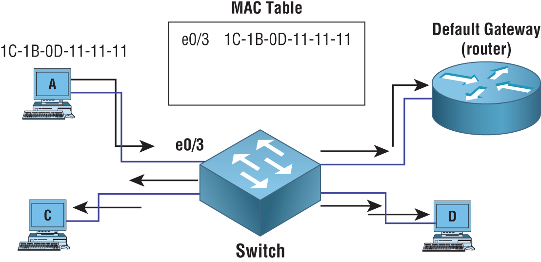
FIGURE 4.1 Switch dynamically learning MAC addresses and ports
Here’s a quick overview of switch operations:
- Initially, the MAC table is empty.
- PC A on port 3 sends traffic to the default gateway.
- The switch caches the MAC address of PC A and its source port.
- Since the switch has not yet learned the default gateway's MAC and port, the frame is flooded out all ports except port 3.
- When the default gateway responds, its MAC and port will be recorded in the MAC table and all traffic between the two going forward will be directly switched.
In the days before switches (and their predecessors, bridges), we used hubs, which had no intelligence. They simply repeated the traffic out all ports, with the exception of the ingress port, taking up bandwidth and CPU of every connected device. If the switch shown in Figure 4.1 were to be replaced with a hub, there would be no MAC table construct since hubs do not have the ability to store MAC addresses. All traffic would be flooded to every device with every transmission.
However, a switch quickly learns the MAC addresses of the devices along with the ports to reach them. If PC A sent a 20GB .MP4 file to PC D, no other device connected to the switch would have their resources affected.
vSphere Standard Switch (vSS)
VMware has three types of virtual switches: the vSphere Standard Switch (vSS), the virtual Distributed Switch (vDS), and the Logical Switch. This can be confusing at first, so we will examine each to get a better understanding.
The vSS works much like a physical switch (see Figure 4.2). Virtual machines connected to it can communicate with one another, and it will forward traffic based on learned MAC addresses. What sets this apart from the other two types of VMware virtualized switches is that it functions on a single ESXi host.

FIGURE 4.2 A vSS can only span a single ESXi host.
A vSS is automatically created by default when ESXi is installed, and each vSS is managed independently on each ESXi host. Like a physical switch, it can also be optimized with traffic shaping, configurable security features, and NIC teaming.
Traffic Shaping
Traffic shaping helps to avoid congestion by effectively managing available bandwidth. As an administrator, you can configure average rate, peak bandwidth, and burst size for a port group. Any VM belonging to that port group will have its traffic shaped according to the limits you define (see Figure 4.3).
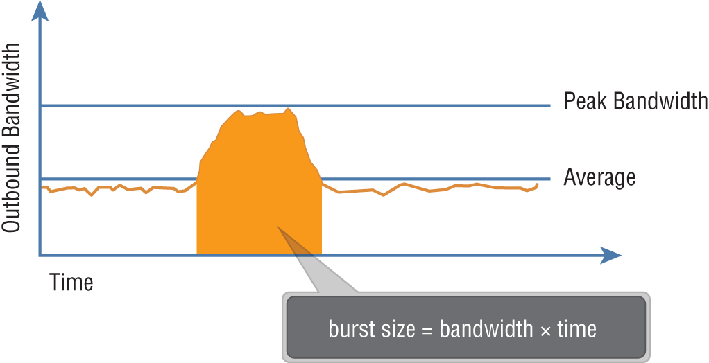
FIGURE 4.3 Traffic shaping is a mechanism for controlling a VM's network bandwidth.
Understanding Port Groups
To understand the function of a port group, begin by imagining ports on a virtual switch. A physical switch in comparison has a fixed number of physical ports; but with a virtual switch, you could have 100 or even 1000 virtual ports. Port groups are essentially templates that allow us to create virtual ports that share a policy. The policy can, for example, enforce rules regarding security and traffic shaping. The most common use is to create a port group for each VLAN. VMs that are connected to the same port group would then belong to the same subnet.
To enable a virtual machine to communicate with the network, you are essentially connecting the VM's virtual adapters to one or more port groups (see Figure 4.4).
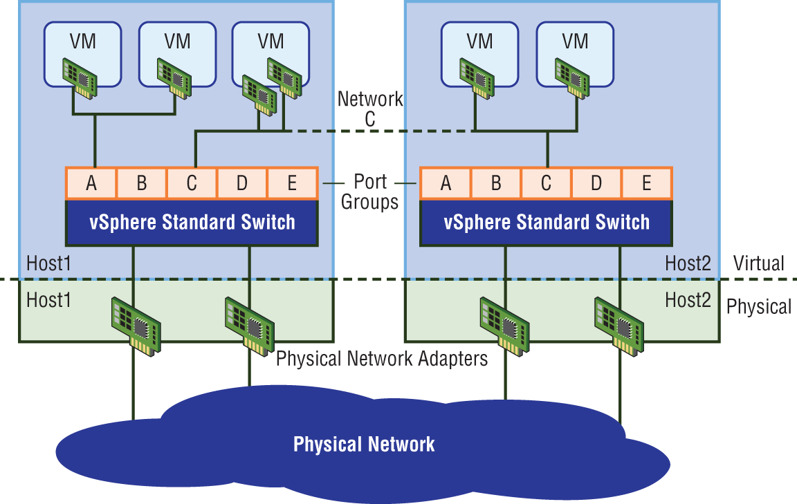
FIGURE 4.4 Port group C has been created on a separate vSS for each ESXi host. All VMs connected to port group C will be in the same subnet.
Each port group is identified by a network label. Whether or not to assign a VLAN ID is optional. You can even assign the same VLAN ID to multiple port groups. For example, let's say you had a set of VMs all on the same subnet, but you wanted the first half of the VMs to use one set of physical adapters to exit the ESXi host in an active/standby configuration, while the second half uses the same physical adapters, but with active and standby reversed. By varying the active/standby status across the two groups, you've improved link aggregation and failover.
Port groups are particularly beneficial to vMotion (see Figure 4.5). When migrating a VM from one host to another, the associated port group contains all the settings for the switch port, making the VM portable. This allows the VM to have the same type of connectivity regardless of which host it is running on.
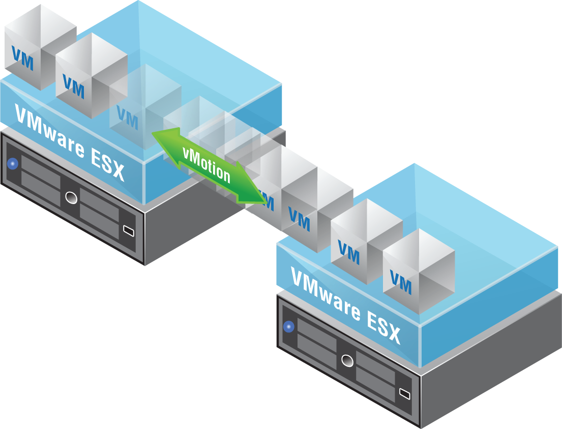
FIGURE 4.5 vMotion not only migrates the virtual machine, but the VM's port group settings such as the IP subnet it belongs to as well.
NIC Teaming
NIC teaming is a feature that allows you to connect a virtual switch to multiple physical network adapters on the ESXi host so that together as a team, they can share the load of traffic between physical and virtual networks (see Figure 4.6). Load balancing increases throughput, and there are several ways to optimize exactly how the load balancing decisions are made and traffic is distributed.
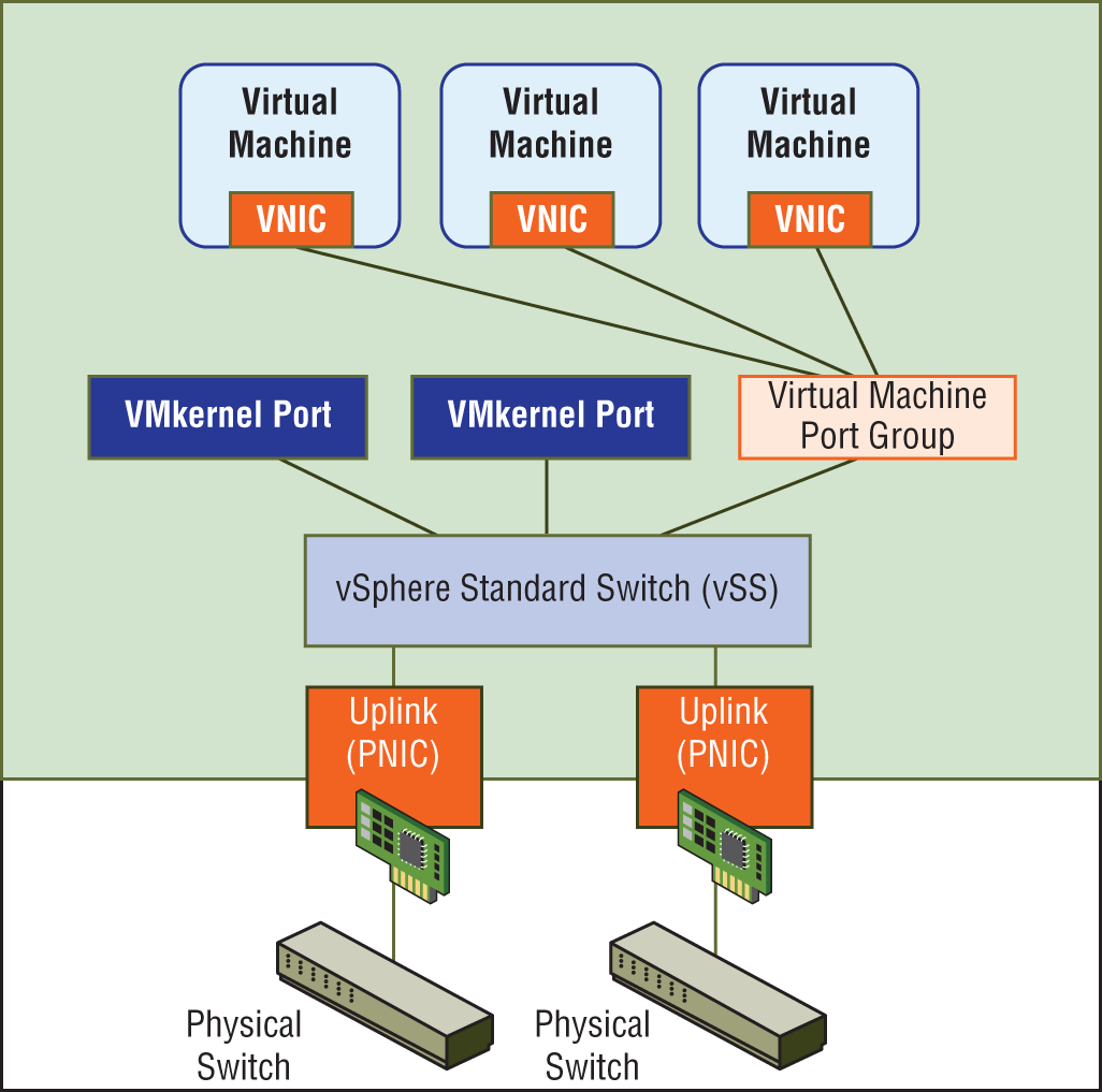
FIGURE 4.6 Connecting the virtual switch to two physical NICs on the ESXi host provides the ability to enable NIC teaming to share the traffic load or provide passive failover.
In addition to increased network capacity, NIC teaming also provides failover. If one of the adapters in the NIC team goes down, Network Failover Detection kicks in to let the ESXi host know that traffic should be moved to the other link.
The NIC teams can be configured as active/active or active/standby. An adapter in standby is only used if one of the active physical adapters is down.
The physical network adapters on an ESXi host are known as uplinks (again, see Figure 4.6). Their job is to connect the physical and virtual networks. On the physical side, they connect to ports on an external physical switch. On the virtual side, they connect to virtual uplink ports on the virtual switch. The virtual switch doesn't use the uplinks when forwarding traffic locally on the same ESXi host. Physical network adapters also go by a couple of other names: vmNIC or pNIC, a real physical interface on an ESXi host.
pNIC is easy to remember since it simply stands for physical NIC. The term vmNIC is often confused at first with other terms we haven't yet introduced: vNIC (virtual NIC), vmkNIC (VM kernel NIC), and vPort (virtual Port). For now, we'll just focus on the physical network adapter found on the ESXi host. It goes by three names: uplink, vmNIC, or pNIC. Also keep in mind that the terms “uplink” and “uplink port” are different. Uplink is the physical network adapter, and uplink port is the virtual port it connects to in the virtual environment.
Ensuring Security
To mitigate Layer 2 attacks such as MAC spoofing and traffic sniffing, several security options are available for the vSphere Standard Switch. One policy option is called MAC Address Changes. When enabled, it allows the guest OS of a virtual machine to define what MAC address it will use for inbound traffic. The initial address of the VM is defined in the
.vmx configuration file (a VMX file is the primary configuration file for the virtual machine) and acts as the Burned In Address (BIA).
When the VM is powered on, the OS of the VM assigns what is called the effective address to the virtual NIC of the VM. Typically, it just copies the initial address and makes it the effective address. However, with a VM powered off, it's possible to change the MAC address. If MAC Address Changes is set to Accept (which is the default), you're allowed to edit it. If it's set to Reject, the OS compares the initial address with the effective address, sees that they are different, and blocks the port. To prevent MAC spoofing (both malicious and otherwise), set the MAC Address Changes option to Reject.
However, there are some cases where you want two VMs to share the same MAC address; for example, with Microsoft Network Load Balancing in Unicast Mode. To allow the MAC address to be modified, you would want the policy to Accept the differing address.
MAC Address Changes are as follows:
- Reject If you set the MAC Address Changes to Reject and the guest operating system changes the MAC address of the adapter to anything other than what is in the
.vmxconfiguration file, all inbound frames are dropped.- If the Guest OS changes the MAC address back to match the MAC address in the
.vmxconfiguration file, inbound frames are passed again.
- If the Guest OS changes the MAC address back to match the MAC address in the
- Accept Changing the MAC address from the Guest OS has the intended effect. Frames to the new MAC address are received.
Another available policy option is Forged Transmits. It is similar to MAC Address Changes in that it also compares the initial address to the effective address and can be configured to Accept or Reject if they are not identical. The difference is the direction of the traffic. The MAC Address Changes policy examines incoming traffic. The Forged Transmits policy examines outgoing traffic.
Forged Transmits are as follows:
- Reject Any outbound frames with a source MAC address that is different from the one currently set on the adapter are dropped.
- Accept No filtering is performed, and all outbound frames are passed.
A third policy option to combat Layer 2 attacks is Promiscuous Mode. Typically, a virtual network adapter for a guest OS can only receive frames that it's meant to see. This includes unicasts, broadcasts, and multicasts. But say, for instance, that you wanted to monitor traffic between two VMs. The switch will do its job and directly switch traffic only between the two VMs. Your sniffer wouldn't be able to capture that traffic. However, if the guest adapter used by the sniffer is in Promiscuous Mode, it can view all frames passed on the virtual switch, allowing you to monitor traffic between the VMs. Unlike the other two security policies mentioned, Promiscuous Mode is disabled by default.
Promiscuous Mode works as follows:
- Reject Placing a guest adapter in Promiscuous Mode has no effect on which frames are received by the adapter.
- Accept Placing a guest adapter in Promiscuous Mode causes it to detect all frames passed on the vSphere standard switch that are allowed under the VLAN policy for the port group that the adapter is connected to.
Virtual Distributed Switch (vDS)
Recall that vSphere Standard Switches are configured individually per host and only work within that host. By comparison, a virtual Distributed Switch (vDS) is configured in vCenter and then distributed to each ESXi host (see Figure 4.7). One of the most salient benefits is centralization. The vDS provides a centralized interface that you can use to configure, monitor, and manage switching for your virtual machines across the entire data center instead of requiring you to configure each switch individually.
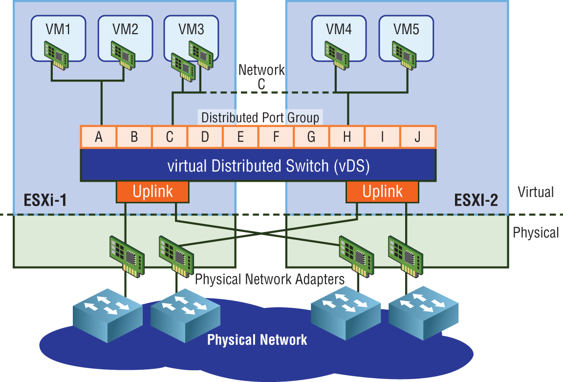
FIGURE 4.7 The vDS is created and managed centrally but spans across multiple hosts.
The key difference between the vSS and the vDS is the architecture. A vSphere Standard Switch Standard Switch contains both the data plane and management plane. You may recall from an earlier chapter that the data plane is responsible for switching traffic to the correct port, whereas the management plane is all about providing instructions for the data plane to carry out. Since both planes are housed together in a vSS, each switch has to be maintained individually.
The architecture of a vDS is different. Each individual switch forwards data via the data plane, but here the management plane is not bundled in. It's centralized, separate from the vDS. This architecture means that instead of having independent switches per host, the vDS abstracts all of the host-level switches into one giant vDS that can potentially span across every ESXi host in the data center.
Centralized configuration also means that it's simpler to maintain and less prone to configuration mistakes. Imagine doing something as simple as adding a port group label to 50 vSphere Standard Switches on 50 ESXi hosts. The chances that you may accidentally misspell the port group label on a few are fairly good, not to mention the time it will take to complete. With a centralized configuration, you define the port group only once and it gets pushed to every host. In addition, centralization also makes troubleshooting easier and less time-consuming.
Simplified management is not the only benefit with vDS. Virtual Distributed Switches also provide features that go beyond the capabilities of a vSphere Standard Switch including:
- Health checks of all uplink connections to detect misconfigurations between the physical switch and the port groups
- vSphere Network I/O Control (NIOC) for categorizing traffic into network resource pools with each pool configured with policies to control bandwidth for the different types of traffic
- Port mirroring to send a copy of traffic from one port to another
- Private VLANs, which are essentially VLANs within VLANs, that can filter traffic between devices on the same subnet, despite not involving a router
- Link Aggregation Control Protocol (LACP) to bundle vmNICs together for load balancing
Virtual eXtensible LANs (VXLANs)
Looking at NSX from a high-level, it's basically an overlay of software that sits on top of your existing physical network (the underlay), abstracting network functions traditionally provided by independently operating devices. This gives enormous flexibility to control and manage what's going on in the overlay, far beyond what was previously possible. The physical network then only needs to provide the plumbing, acting as a simple pipe that physically carries traffic from host to host.
Using the NSX overlay removes a lot of the complexities we see in traditional underlay (physical) environments. Configurations on core data center devices go from hundreds of pages down to 20 or less in many cases.
It also allows us to have, for example, VM1 on ESXi host 1 to be on the same segment, same subnet as VM5 on ESXi host 2. If all your hosts were interconnected with physical switches, the extension of a single subnet across hosts is easy to imagine since switches allow you to extend a subnet. But what if a host had to send traffic through a physical router to reach another host? (See Figure 4.8.)
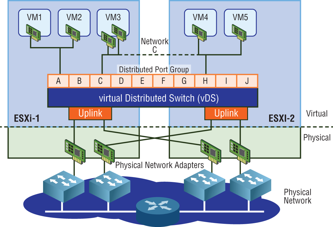
FIGURE 4.8 Traffic from ESXi-1 to ESXi-2 in this topology must now traverse a Layer 3 boundary: a router.
Switches can extend a network segment, but routers terminate segments. Routers create Layer 2 boundaries. Therefore, every interface on a router belongs to a different subnet/segment. For example, you could not have the IP 10.1.1.1 /24 configured on one interface and 10.1.1.2 /24 on another interface of the same router. A router's job is to connect different segments (different subnets) and to determine the best path to reach remote segments.
NSX doesn't care if the physical network is made up of routers or switches interconnecting the ESXi hosts. Instead, the way host-to-host connectivity works is through tunneling. Recall the subway analogy from Chapter 2. The physical network is treated like a subway that NSX uses to get from building to building (host to host). Each ESXi host has a subway stop, which is simply a tunnel endpoint. These are referred to as a Virtual Tunnel Endpoints (VTEPs). See Figure 4.9.
Tunneling is simply taking the traffic we want to send, breaking it into pieces, and encapsulating it inside an Ethernet frame by adding an additional header containing the “subway stop” information. Once the traffic is received at the destination tunnel endpoint, the header is stripped off and the packet decapsulated. What's left is the original frame that was sent from the source. The VXLAN header adds an additional 50 bytes of overhead to the Ethernet frame (see Figure 4.10). The default Maximum Transmission Unit (MTU) size for an Ethernet header is 1500 bytes. To accommodate the larger frames used for VXLAN traffic, the MTU size should be configured to support 1600 bytes at a minimum.
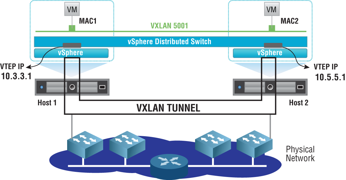
FIGURE 4.9 Two VMs on the same subnet but located on different hosts communicate directly regardless of the complexity of the underlying physical network by tunneling to the VTEP of the remote ESXi host.
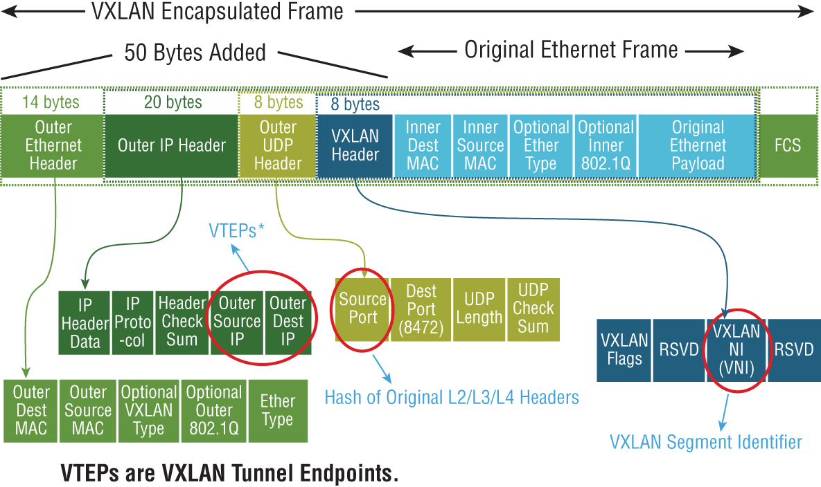
FIGURE 4.10 The original frame generated from the source VM is encapsulated inside a VXLAN frame by adding a 50-byte header containing the information required to tunnel the traffic to the destination VTEP.
Jumbo frames are simply Ethernet frames that carry more than a 1500-byte payload. When using jumbo frames on the virtual side, the underlay also needs to account for this. For this reason, it is recommended to use an MTU 9214 or 9216 byte size, depending on vendor support for your underlying physical devices. Also be aware that some devices require a reboot for the new MTU size to take effect (Cisco switches, Palo Alto firewalls, etc.). Therefore, some planning is required.
Each network physical adapter on an ESXi host gets a VTEP assigned to it. It is the VTEP that is responsible for both encapsulating traffic as it exits an ESXi host and for decapsulating traffic that is received. The VTEP is a special VM kernel interface that has its own IP address (see Figure 4.11).

FIGURE 4.11 Using the analogy of a subway stop, for VM1 to send traffic to VM3, the traffic is tunneled to stop 10.2.2.1, the IP of the VTEP on the third ESXi host.
The host has a table indicating which VTEP address (which “subway stop”) should be used when sending traffic to a remote VM. That IP information is included in the VXLAN header. VXLAN traffic is identified with UDP port 8472 for any NSX installation starting with version 6.2.3.
If you are familiar with VLAN tagging, the idea is very similar. VLAN tagging is another example of encapsulation. Its job is to encapsulate frames and add a VLAN ID so that when a remote switch receives a tagged frame, it knows to send the frame out ports that belong to the same VLAN. Once the destination VLAN has been determined, the packet is decapsulated, discarding the header, and the destination device receives the unaltered frame sent by the source.
VXLAN is an encapsulation technique that was originally developed by VMware, Cisco, and Arista and was eventually documented in RFC 7348 to standardize an overlay encapsulation protocol. It allows you to extend a Layer 2 domain through Layer 3 boundaries (routers).
Employing Logical Switches
With NSX, you can spin up a Layer 2 network just as easily as a virtual machine. Because the physical network infrastructure is decoupled from the logical VXLAN overlay network, the endpoints connecting to the L2 segment can be anywhere in your data center when using a Logical Switch in NSX
From the perspective of the ESXi host, a Logical Switch is a port group on a vDS. Without a vDS, you can't create a Logical Switch. The term itself can be confusing, especially if you are trying to contrast it with a physical switch. A physical switch can carry many VLANs. The traffic from each VLAN is a different subnet. A Logical Switch instead is more like a single subnet (a single VLAN.) It makes more sense that a Logical Switch would only represent a single VLAN rather than attempting to emulate a single physical switch supporting thousands of VLANs because it is virtual. In the physical world, you wouldn't necessarily purchase a dedicated switch for every VLAN. There is often some consolidation to lower cost. Since the Logical Switches are entirely virtual, cost is not a factor, so it's simpler to create one for each workload. In terms of function, the Logical Switch is much more flexible than a physical switch because it lives on a virtual Distributed Switch. This means that it can potentially extend to all ESXi hosts. Therefore, VM 10.1.1.1 can communicate directly with VM 10.1.1.2 regardless of where their respective hosts are located within the data center and regardless of how many routers separate them.
Virtual machines attached to a Logical Switch are connected by VXLAN virtual wires. These appear on the virtual Distributed Switch. When you deploy a new Logical Switch in NSX, a port group is automatically created on the vDS and its name will contain the word virtualwire along with a number between 5000 and 16,777,215 (see Figure 4.12).
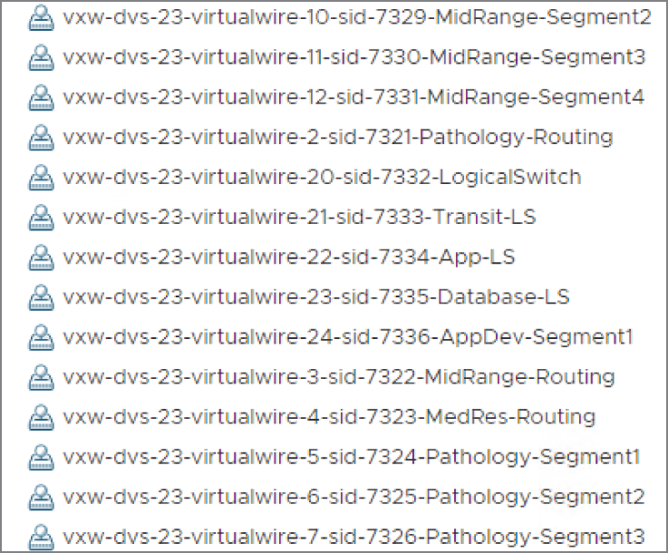
FIGURE 4.12 Each Logical Switch created receives an ID from the segment pool and a virtual wire. The virtual wire is a port group created on the vDS.
These segment IDs are defined in a pool with a range defined. A typical pool might be set with a range from 5000 to 6000. For example: vxw-dvs-311-virtualwire-sid-5001-app. In the virtual environment, instead of referring to this number as a VLAN ID, it's called a VXLAN Network Identifier (VNI) Network Identifier (VNI). Keep in mind that the Logical Switch is like a single VLAN that only exists in the virtual environment and is labeled with a VNI number. If you have a background in networking, you already are aware that a VLAN is a single subnet. The same idea applies here. Each VNI represents a different subnet.
If the term Logical Switch is still a point of confusion, substitute the word “Overlay” for “Logical” here. It is an Overlay Switch. It only exists in the NSX overlay and it represents a single L2 segment, but with the added ability to extend across the entire data center. Physical switches not only lack that extensibility, they also must play by the rules of VLANs. For example, in a VLAN header, the VLAN ID field is 12 bits, which gives a maximum of 4096 combinations (see Figure 4.13).
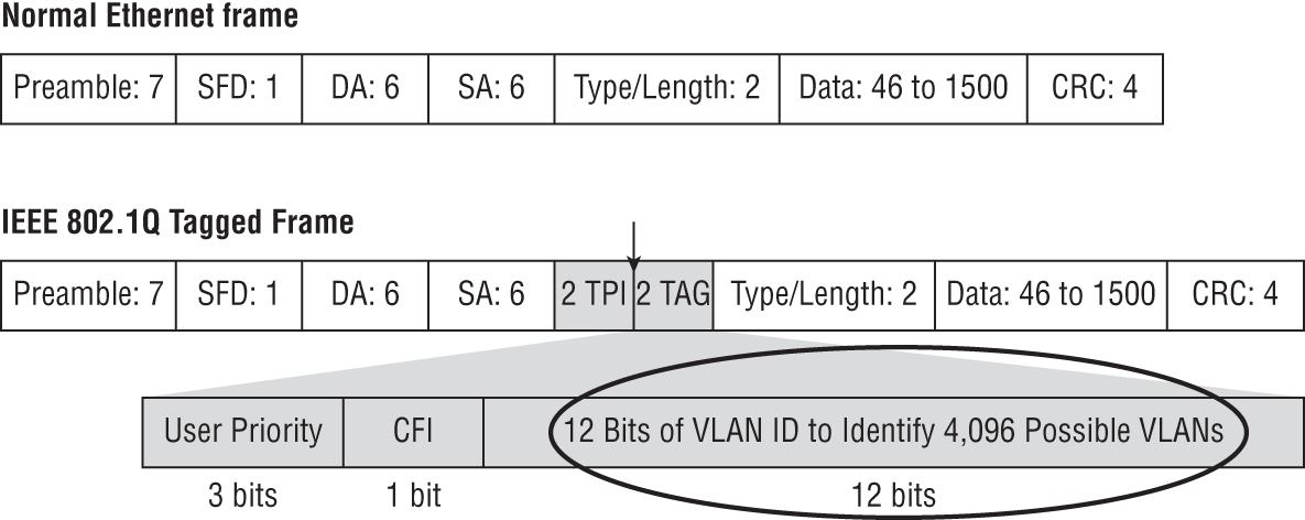
FIGURE 4.13 The VLAN ID field is 12 bits long, which indicates that over 4000 VLAN IDs can be created from the 12-digit combinations of ones and zeros.
The Overlay Switch uses VNIs, which gives us over 16 million numbers to choose from, meaning that theoretically, you could have over 16 million subnets. For almost all enterprise networks, they will never even come close to the 4000+ VLAN limitation. However, for service providers with thousands of customers, it's a different story. VLAN IDs and VNIs are close cousins, but VNIs are much more scalable.
Consider another benefit of a Logical Switch over its physical counterparts. If you have 100 physical switches and want to add a new Layer 2 domain, all 100 must be configured individually to support it. With NSX, adding that new Layer 2 domain only requires creating a new Logical Switch, and it only needs to be done once. It is just as simple to delete a Layer 2 domain. As an administrator, if you needed any two VMs in your data center to communicate directly ad hoc, a Logical Switch can be quickly and easily created to provide that connectivity and can, just as quickly and easily, be torn down when the job is complete.
After a Logical Switch is created, all members of the same Transport Zone have access to it. A Transport Zone is simply a collection of VTEPs that can share VNI information. The VTEP knows which VMs are located on each ESXi host and what segments the VMs are attached to. The information is shared with every VTEP in the same Transport Zone (see Figure 4.14).

FIGURE 4.14 Each VTEP, indicated here with an IP address starting with 192.168.X.X, can be viewed as a door to an ESXi host.
Transport Zones were originally created to support different overlay encapsulation types. Each encapsulation type would use a different zone. With NSX-V, a decision was made to only use one encapsulation type: VXLAN. Most implementations will use a single transport zone. The exception is when using a Universal Transport Zone that only comes into play with Cross-vCenter, which allows us to tie multiple vCenter Servers together.
Three Tables That Store VNI Information
To communicate at Layer 2, a Layer 2 address (a MAC address) is needed. Not only do your VMs have MAC and IP addresses, but the VTEPs do as well. On a physical switch, an attached server sends its first frame, and the switch records the MAC address, its associated port, and the VLAN it belongs to in its MAC table. This information is maintained in the table for 300 seconds (5 minutes). During that time, if the switch receives any traffic destined for the server's MAC address, it knows exactly which switch port the server is plugged into. Armed with this information, the switch can forward the traffic directly to the server and only the server. MAC tables on physical switches map learned MAC addresses to physical ports. With a Logical Switch, there are no physical ports, so the MAC table in NSX behaves a bit differently.
Collecting
VNI Information
In NSX, three tables hold Virtual Network Information: the VTEP table, the MAC table, and the Address Resolution Protocol (ARP) table. The function and behavior of each is easier to understand with an example (see Figure 4.15).

FIGURE 4.15 VM-A is attached to VXLAN 5001. When it is powered on, information about VNI 5001 is then populated in three tables: the MAC table, the VTEP table, and the ARP table.
In this scenario, there are two VXLANs: VNI 5001 and VNI 5002. If you take a closer look at the virtual machines attached to these segments, you'll see that VNI 5001 is on subnet 10.1.1.X and VNI 5002 is on subnet 192.168.1.X. If we want information about VNI 5001, we can use these three CLI commands to look at the MAC, VTEP, and ARP tables:
show logical-switch controller master vni 5001 macshow logical-switch controller master vni 5001 vtepshow logical-switch controller master vni 5001 arp
Assuming all the VMs were powered off, the tables would be empty.
We then power on VM-A. VTEP-1 takes note and populates its local MAC table with the MAC address of VM-A (00:50:56:AA:AA:AA) and the VNI segment it is attached to (VNI 5001) along with the VTEP's own IP (172.16.1.1). The VTEP is like a door to the host, and it's aware of all VMs that live behind that door. The mapping here of VM-MAC to VTEP-IP is so that other VMs know which door to go to in order to get to VM-A. We can view the MAC table with the following command:
show logical-switch controller master vni 5001 macTraffic coming from another VM on a different host would need to know the IP of the door (VTEP) to go through to reach VM-A. The answer is 172.16.1.1, the VTEP IP. However, the IP address isn't enough. We would also need to know the Layer 2 (MAC) address of the VTEP. That information isn't stored in the MAC table; it's stored in the VTEP table. An example is shown in the middle column of Figure 4.15.
There, you will see for VNI 5001 the mapping of the VTEP IP to the VTEP MAC address. We can view the VTEP table for VNI 5001 with the following command:
show logical-switch controller master vni 5001 vtepIn the last column of Figure 4.15, you see the IP address of VM-A and that it is associated with VNI 5001. Just like it was necessary to know the Layer 2 address associated with the VTEP's IP address, the same applies to the IP address of the VM itself. The mapping here is built by Address Resolution Protocol (ARP). We'll get into the details of that process coming up, but for now, just be aware that for a packet to be sent to VM-A, we need to know both its Layer 3 (IP) and Layer 2 (MAC) addresses. The ARP table can be viewed with the following command:
show logical-switch controller master vni 5001 arpCentralized MAC Table
The VNI information collected by the VTEP is sent to the NSX Controller cluster. The Controller cluster then shares the information with every VTEP on each ESXi host within the same Transport Zone. Since every VTEP is doing the same, the Controller cluster is able to collect and disperse all of the VNI information for the entire Transport Zone, ultimately meaning that if every VTEP in the data center falls within the same Transport Zone, each has all the information it needs to know exactly where every VM is located and how to get there (see Figure 4.16).

FIGURE 4.16 VTEPs send their local VNI information to the Controller cluster, where it is distributed to the other VTEPs in the same Transport Zone.
With the tables populated, let's walk through the process again. We want to send a packet to VM-A. We know that VM-A's IP address is 10.1.1.1. Looking at the ARP table (see Figure 4.17), we see that the MAC address associated with 10.1.1.1 is 00:50:56:AA:AA:AA. This MAC address can be found behind one of the VTEPs. The MAC table is checked, and we find that the MAC of VM-A (00:50:56:AA:AA:AA) is behind VTEP 172.16.1.1. We want to send the packet to the correct VTEP, but all we have is the IP address so far. To find its associated MAC address, we examine the VTEP table. There we find that the MAC address associated with VTEP 172.16.1.1 is 11:11:11:11:11:11.
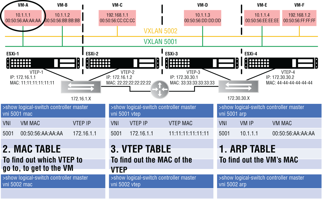
FIGURE 4.17 Walkthrough to find the VNI information needed to send traffic to VM-A
Now that you know the purpose of each table, let's power on another VM and see what changes.
VTEP Table
VM-B is located on ESXi-1 (see Figure 4.18). As long as it is powered down, we have no related information in any of the three tables. Let's examine how each table changes once the virtual machine comes online.

FIGURE 4.18 VNI information added when VM-B is powered up
Looking at the MAC table (first column), we see that the VTEP recorded VM-B's MAC address and entered its own VTEP IP (172.16.1.1).
Looking at the ARP table (third column), we see that the VTEP recorded the IP and MAC of VM-B.
But, why isn't there any new information added for the VTEP table (second column)? The reason is that both VM-A and VM-B sit behind the same door, VTEP-1 (172.16.1.1). This table simply records the IP-to-MAC mapping of the VTEP. Since this mapping (172.16.1.1=11:11:11:11:11) was recorded previously, there's nothing new to add to the table.
Now, let's power on VM-D and check the tables again (see Figure 4.19).
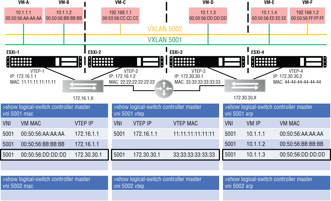
FIGURE 4.19 VNI information added when VM-D is powered up
The MAC table (first column) records which VTEP (172.30.30.1) is the door to VM-D (00:50:56:DD:DD:DD).
This time, the VTEP table (second column) has new information. The reason is that VM-D isn't located on ESXi-1 like the previous two VMs. It is on ESXi-3, behind VTEP-3 (172.30.30.1). The previously recorded VTEP entries were for ESXi-1's VTEP-1 (172.16.1.1).
The VTEP table records the associated VTEP-3 MAC address (33:33:33:33:33:33). If VM-A (10.1.1.1) were to communicate with VM-D (10.1.1.3), it's on the same segment/subnet from VM-A's perspective. VTEP-1 must send the traffic through the physical router shown in the middle to reach VTEP-3. Even though we are crossing a Layer 3 boundary, this is the magic of having an overlay. The network as seen from the virtual side is simpler. VM-D is just another VM on the same segment; but in reality, the traffic is being tunneled through the physical network, exiting one tunnel endpoint (VTEP-1) to leave the virtual environment and re-entering the virtual environment on a different host using another tunnel endpoint (VTEP-3).
The ARP table has VM-D's IP-to-MAC mapping.
Now that you have a better understanding of the process, let's power on one more VM and see what changes.
We power on VM-F (see Figure 4.20).
Examine the first column, showing the MAC table. A key thing to note here is that this new information is not stored in the VNI 5001 MAC table, it's stored in the VNI 5002 MAC table. Why not just have one big MAC table like we see in physical switches? It's all about dividing the work and distributing it among the nodes. Remember that the information gathered locally is then sent to the Controller cluster. These three nodes have the same job description, but they divide the work into slices, each taking a slice that corresponds to a different VNI. One slice is all the information gathered for VNI 5001; another slice is the information for VNI 5002. In the example shown in Figure 4.21, Controller 2 is responsible for the tables of VNI 5001, 5004, and 5007. This includes the tables for ARP, MAC, and VTEP.

FIGURE 4.20 Powering on VM-F adds VNI information to a new table.

FIGURE 4.21 The three Controller nodes divide the workload of tracking VNI information.
Ultimately, it all gets propagated to every ESXi host, but the task of collecting and distributing the VNI information is made more efficient by defining which controller keeps track of what information. Additionally, if one of the nodes in the Controller cluster were to fail, the slices for the failed node would be reassigned to the remaining nodes.
We Might as Well Talk about ARP Now
Address Resolution Protocol is used to discover the MAC address (Layer 2) of an endpoint when you already know the IP address (Layer 3). That information is then stored in the previously mentioned ARP table. But how does ARP work to make the discovery?
First, let's look at how a packet travels from point A to B in a physical network and see where ARP fits into the mix; then we'll look at how it works within NSX.
When a PC wants to send a packet, there's not a lot of decision-making going on. It simply needs to figure out whether the destination is local or remote (see Figure 4.22).

FIGURE 4.22 The PC, 10.1.1.3/24, wants to send packets to the server, 30.1.1.9/24.
This is where the subnet mask comes in. If the PC's IP address is 10.1.1.3 with a mask of /24 (255.255.255.0), the mask indicates a match on the first three octets, the first 24 bits. Any destination that starts with 10.1.1.X is local. Everything else is remote.
For example, from the perspective of PC 10.1.1.3, a server with the address 30.1.1.9 would be remote. Since the destination is remote, the PC needs to forward the packet to its default gateway. Gateway is simply an older term for router. Your default “router” is your gateway out of the local subnet. For the PC's traffic to reach the server, it must leave the local subnet. In this example, R1 is the PC's default gateway, 10.1.1.4.
Before your PC sends the frame to the gateway, all source and destination fields for both Layer 2 and Layer 3 headers need to be filled in. You can't send a packet with partially filled in headers. For Layer 3, that's easy to determine for the PC. The source IP belongs to the PC itself, 10.1.1.3. The destination IP is the server receiving the data, 30.1.1.9. The source MAC address is immediately known because it also belongs to the PC. The only piece missing is the destination MAC address, but this is not the MAC address of the server, your final destination. It is the MAC address to get across the local link. It is the MAC address of your default gateway.
LAYER 2 HEADER LAYER 3 HEADER_______________ 0000.0000.1111 10.1.1.3 30.1.1.9dest mac source mac source IP dest IP
Filling In the L2 and L3 Headers
We may have to traverse several data links (local links) to get to the destination. In the Figure 4.22 diagram, we have three links to cross: the link from the PC to R1, the link from R1 to R2, and the final link from R2 to the server.
This is where ARP comes in to help. The PC knows the IP address of its default gateway on the local link but has no clue what MAC address that router is using (see Figure 4.23). To send the packet across the local link, it must also learn the default gateway's MAC address.
It essentially broadcasts the message, “Whoever has the IP address 10.1.1.4, please tell me your MAC address.” Being a broadcast, it is picked up by every device on that subnet. However, only the device with that IP, which in this case is R1, responds with a unicast. “Yes, I'm 10.1.1.4 and my MAC address is 0000.0000.aaaa.”
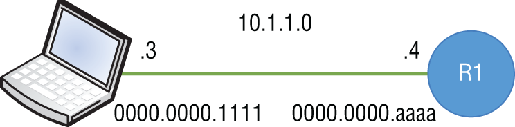
FIGURE 4.23 The PC knows the default gateway IP address 10.1.1.4 through DHCP or manual configuration.
The PC keeps this information in ARP cache for 4 hours (14400 seconds).
Now the final field (the destination MAC) can be filled in and the packet is sent to R1:
LAYER 2 HEADER LAYER 3 HEADER0000.0000.aaaa 0000.0000.1111 10.1.1.3 30.1.1.9dest mac source mac source IP dest IP
R1 knows to pick it up from the wire because it sees its own MAC address as the destination MAC. After doing a Frame Check Sequence (FCS) calculation to make sure the packet has not been changed or corrupted, the router breaks off the Layer 2 header altogether and sends the remainder up to Layer 3, the network layer:
LAYER 3 HEADER10.1.1.3 30.1.1.9source IP dest IP
What remains is the Layer 3 header. The router looks at the destination IP to determine if the destination network is a known route in its routing table. In this example, say we have a routing protocol running on both routers, allowing them to learn all the routes, including network 30.1.1.0. Look back to Figure 4.22 to see the end-to-end network.
The routing table on R1 would show that the next hop toward network 30.1.1.0 is 20.1.1.2 (R2). In the example shown in Figure 4.24, assume that there is an entry and that the next hop to get there is R2: 20.1.1.2.
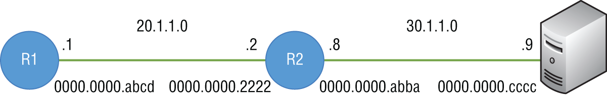
FIGURE 4.24 Once R1 (the PC's default gateway) receives the packet, it checks its routing table to see if there is an entry to know how to get to the destination network, 30.1.1.0.
To get across this data link, though, we need to rebuild a new Layer 2 header with the source being R1's MAC address and the destination being R2's MAC address. The Layer 3 header remains unchanged, with the PC as the source and the server as the destination.
LAYER 2 HEADER LAYER 3 HEADER_____________ 0000.0000.abcd 10.1.1.3 30.1.1.9dest mac source mac source IP dest IP
We have the same issue as before. R1 knows that the next hop IP address is 20.1.1.2, but it has no idea what R2's associated MAC address is. So again, it ARPs. “Whoever has the IP address 20.1.1.2, please tell me your MAC address.” R2 responds with, “Yes, I'm 20.1.1.2 and my MAC address is 0000.0000.2222.”
R1 fills out the remaining field (destination MAC) in the Layer 2 header, which allows it to cross the local link:
LAYER 2 HEADER LAYER 3 HEADER0000.0000.2222 0000.0000.abcd 10.1.1.3 30.1.1.9dest mac source mac source IP dest IP
R2 receives the frame and picks it up from the wire since it sees its own MAC address as the destination at Layer 2.
The same process is repeated for the final link to the server. R2 checks its routing table to see if it can reach network 30.1.1.0 and finds that it is directly connected. It then goes through the same ARP process as in previous steps to determine the MAC address of the server, 30.1.1.9 (see Figure 4.25).
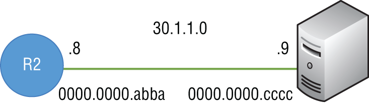
FIGURE 4.25 The destination network, 30.1.1.0, is directly attached.
The Layer 2 header is stripped off, the routing table is checked to see if it has a route to 30.1.1.0, and then seeing that 30.1.1.0 is directly connected, R2 rebuilds a new Layer 2 header with the server's MAC address, 0000.0000.cccc, as the destination and R2's MAC address, 0000.0000.abba, as the source.
The server receives the frame and sends the data all the way up the stack to Layer 7.
That's how it works in the physical networking world. Now let's see how NSX improves on the idea.
Switch Security Module
ARP broadcast traffic can consume a lot of resources. It's not only bandwidth; CPU resources are consumed when sending requests and also when recording the information received. To lessen the impact, NSX Logical Switches can suppress ARP flooding between VMs that are connected to the same Logical Switch. This feature can be disabled per Logical Switch. If you wanted VNI 5001 to have ARP suppression functionality and 5002 to not have it, as an administrator, that option is provided by the Switch Security module of the Logical Switch. Although it can be disabled, the ability to suppress ARP broadcasts is a key feature in NSX that helps to scale in large domains.
Using a previous topology, let's say that VM-A (10.1.1.1) needs to send traffic to VM-E (10.1.1.4). They both are connected to the same Logical Switch: VNI 5001. Examining the diagram in Figure 4.26, you'll see that they are both on VXLAN 5001, subnet 10.1.1.X, the same local link.
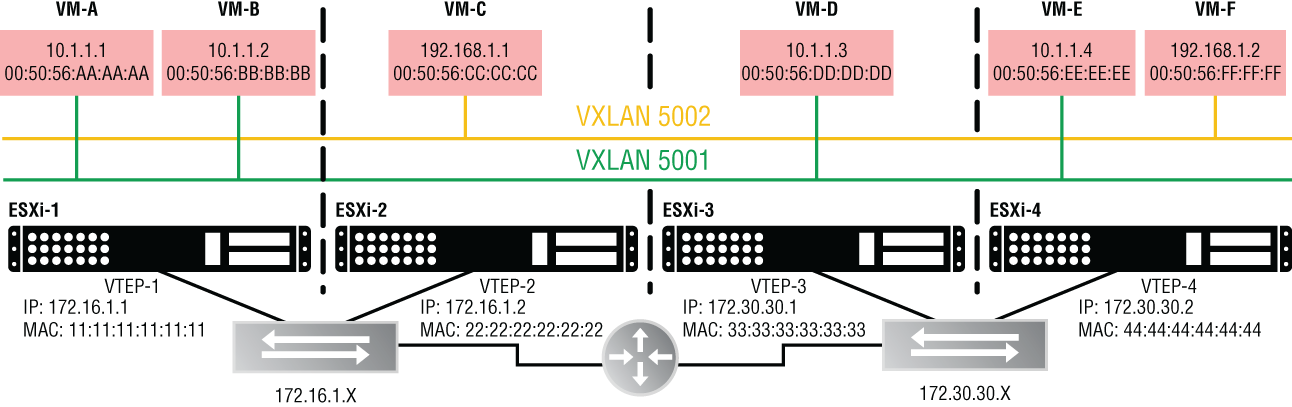
FIGURE 4.26 VM-A needs to send packets to VM-E.
VM-A has no idea it's a virtual machine. It behaves the same as a physical PC. From VM-A's perspective if we are assuming it has a subnet mask of 255.255.255.0, it's on the 10.1.1.X network. It is attempting to send traffic to 10.1.1.4 and by applying the mask, it sees that there's a match. Both the source and destination are on the same 10.1.1.X network. Although it knows the destination IP of VM-E, 10.1.1.4, it has no clue what VM-E's MAC address is, so it sends an ARP request as a broadcast.
The Switch Security module of the Logical Switch intercepts the broadcast and checks to see if it has cached the requested ARP information. If it already has an ARP entry for the destination, it immediately sends that information to VM-A as a unicast and the broadcast is suppressed, not taking up bandwidth or CPU of any other VM. If the ARP information for the target is not found, the Logical Switch sends a direct ARP query to the Controller cluster. If the Controller cluster has the VM IP-to-MAC binding, it replies to the Logical Switch with the ARP information, which then forwards that response to VM-A.
Initially, there would be no ARP information stored on the Controller cluster about VM-E. When the Controller cluster doesn't have the ARP entry, the ARP request is rebroadcast by the Logical Switch. At this point, all of the VMs on the 10.1.1.X subnet would receive the ARP request, but only VM-E would respond since the message specifies that it is intended for 10.1.1.4. The response is then noted by the Switch Security module, since one of its jobs is to specifically listen in on all ARP conversations. It's equally nosey when it comes to DHCP conversations. Once the Switch Security module has the ARP mapping for VM-E, it notifies the Controller cluster.
At this point, both the Controller cluster and the Switch Security module have the ARP information for VM-E, but what about VM-A? When the initial ARP request was generated from VM-A, included in that request was VM-A's own information regarding its IP address and its MAC address. This information is passed from the Switch Security module to the Controller cluster as well. This means that the Controller cluster and Switch Security module at this point have all the ARP mapping information needed for both VM-A and VM-E, triggered from a single ARP request generated by VM-A.
Understanding Broadcast, Unknown Unicast, and Multicast
When a physical switch receives a unicast, say to 00-00-0C-11-22-33, it checks its MAC table to see if an entry exists for that MAC address, and if so, it indicates which exiting port it should use to forward the frame. With NSX, instead of an exiting port, it would indicate which VTEP to send it to. However, when a physical switch receives a broadcast, there is no mapped port in the MAC table. Instead, it floods the broadcast out all ports in the same VLAN, except for the port it came in on. Remember that a broadcast is essentially addressed to all nodes in that L2 domain. Multicasts are just a subset of broadcasts and are also flooded.
But what if you have an unknown unicast? Let's say that the traffic is destined for 00-00-11-22-33-44, but there isn't an entry for that MAC address in the table yet. The switch doesn't drop the traffic; it floods it the same as it does with broadcasts and multicasts. When other devices in that L2 domain see the frame cross their wire, they won't pick it up because the destination MAC address isn't theirs. The mail isn't addressed to them, so to speak, and therefore they don't touch it. Only the device with a matching MAC address will pull it from the wire and process the frame.
Layer 2 Flooding
All three of these frame types—Broadcast, Unknown unicast, and Multicast (BUM traffic for short)—are treated the same way by the switch. The traffic is flooded. Flooding is another way to say that the traffic is replicated. When two VMs on different hosts communicate directly, the traffic is exchanged between the two tunnel-endpoint VTEP IP addresses without any need for flooding. But when traffic needs to be sent to all other VMs that are connected to the same Logical Switch, this is BUM traffic. It is still considered BUM traffic and is subject to flooding if the VMs are connected to the same Logical Switch but are found on different ESXi hosts. Any BUM traffic that is originated from a VM on one host needs to be replicated to all remote hosts that are connected to the same Logical Switch.
Replication Modes
How this traffic is replicated depends on what we discussed at the end of Chapter 2, “NSX Architecture and Requirements,” regarding replication modes. We pointed out that there are three options: Multicast Mode, Unicast Mode, and Hybrid Mode (see Figure 4.27).
We're bringing it up again since this chapter is all about switching, and the different replication modes affect how the Logical Switch will handle replicating broadcasts, unknown unicasts, and multicasts instead of simply flooding like physical switches do. Now that we've gone into more depth regarding switching behavior, you might want to peek back at those paragraphs covering replication modes in Chapter 2. They should be easier to digest now that you have a broader understanding of how the modes fit in NSX operation.
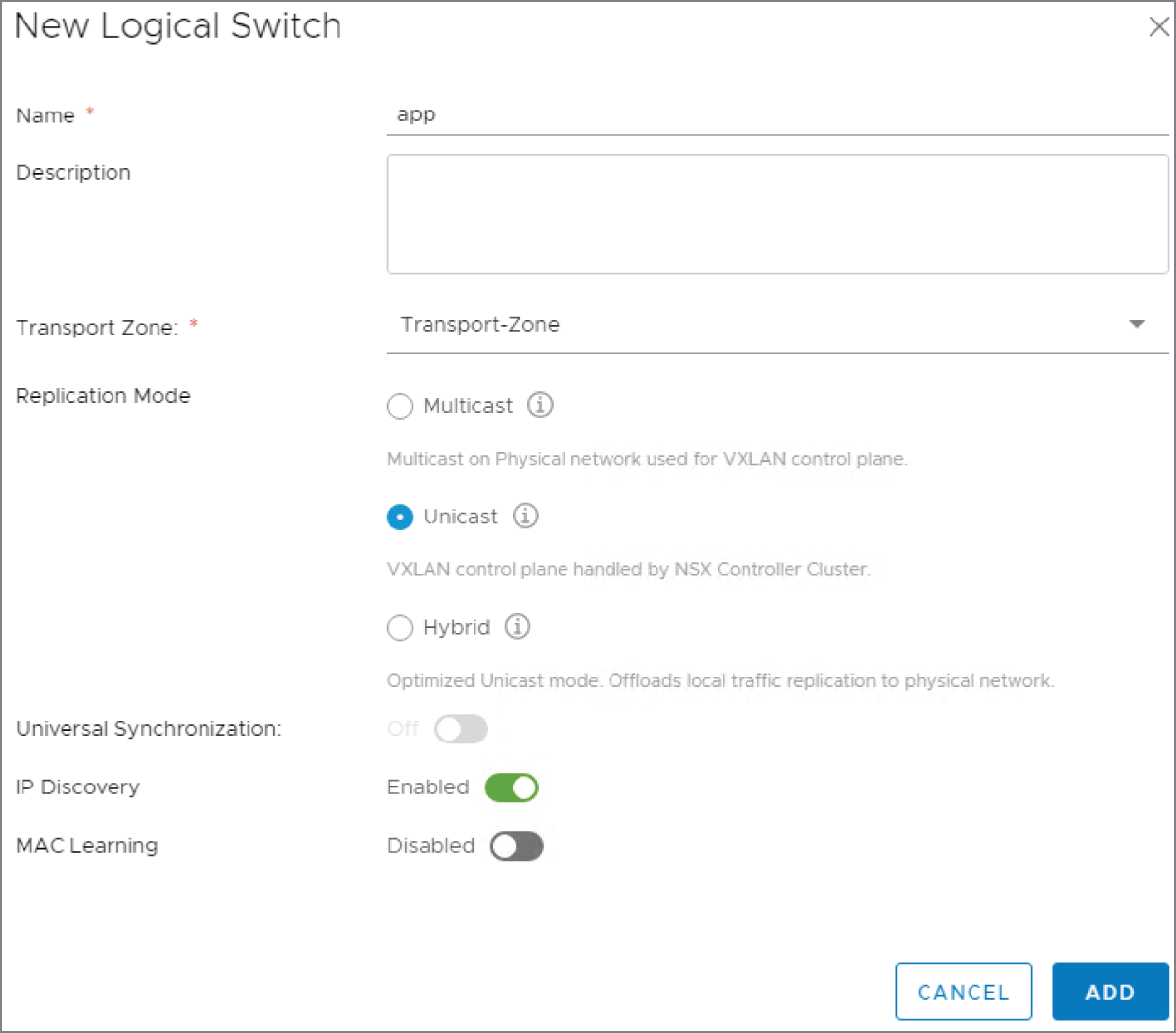
FIGURE 4.27 Selecting a Replication Mode (Multicast, Unicast, Hybrid) when creating a new Logical Switch
Deploying Logical Switches
Earlier in the chapter, we said that Logical Switches are similar to VLANs in the physical environment. You can think of them as Overlay Switches that live in the virtual environment or as switches that only carry one VLAN. Stick with the description that makes the most sense to you. Although Logical Switches can span multiple hosts, they are local to a single vCenter Server NSX deployment. If you want a Logical Switch to span all vCenters in a cross-vCenter deployment, you can create universal Logical Switches. Whether a newly created switch is a Logical Switch or a universal Logical Switch depends on the Transport Zone type you choose when creating it. In the field for Transport Zone, shown in Figure 4.27, when you click Change, you will see the available Transport Zones. Selecting a non-universal Transport Zone will create a regular Logical Switch.
You can also see from Figure 4.27 that in order to create a Logical Switch, you'll need to choose a replication mode and optionally enable IP discovery and MAC learning. By default, IP discovery will minimize traffic caused by ARP flooding when ARP is used to discover the MAC address information between two VMs on the same Logical Switch. MAC learning is an option that creates a table on each virtual NIC to learn what VLAN is associated with what MAC address. This is helpful when working with vMotion. When a virtual machine is moved to a different location, these tables are transported with the VM. The Logical Switch then would issue a Reverse ARP (RARP) for all the entries in the tables.
Creating a Logical Switch
To create a Logical Switch, perform the following steps:
- Open your vSphere client and go to Home ➢ Networking & Security ➢ Logical Switches.
- Select the NSX Manager that will be associated with the Logical Switch.
Remember that the Logical Switch is local to a single vCenter NSX deployment. For a cross-vCenter deployment, create the Logical Switch on the primary NSX Manager.
- Click the green plus sign: New Logical Switch.
- Enter a name for the Logical Switch. The description is optional.
- Select the Transport Zone.
If you select a universal Transport Zone, you will create a universal Logical Switch.
You can select a replication mode (Unicast, Multicast, or Hybrid), but by default the Logical Switch will simply inherit whichever replication mode was previously selected when the Transport Zone was configured.
- To enable ARP suppression, click Enable IP Discovery.
As mentioned previously, you also have the option here to Enable MAC Learning.
Once deployed, you are ready to connect VMs to the Logical Switch.
The Bottom Line
- Address Resolution Protocol Address Resolution Protocol (ARP) is used to discover the MAC address of the next hop along the path.
- Master It You are troubleshooting a connectivity issue (see Figure 4.28). In one of your tests, you ping the server on the right from the PC on the left. Using a packet sniffer, you examine the packet received on the server. If everything is working as it should, what source MAC address do you expect to see in the Layer 2 header?
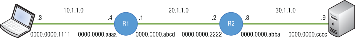
FIGURE 4.28 Troubleshooting connectivity
- Master It You are troubleshooting a connectivity issue (see Figure 4.28). In one of your tests, you ping the server on the right from the PC on the left. Using a packet sniffer, you examine the packet received on the server. If everything is working as it should, what source MAC address do you expect to see in the Layer 2 header?
- VTEP Table The Virtual Tunnel Endpoint can be thought of as a door or subway stop on the ESXi host to the VMs behind it. The VTEPs store the information for every VNI and VM that is local to the host. This information is then sent to the Controllers, which are responsible for distributing the information to all of the other ESXi hosts.
- Master It You are troubleshooting an issue and need to verify that the mappings are correct. You issue the following command:
show logical-switch controller master vni 5001 vtepWhat do you expect to see?
- VNI 5001, the VTEP IP, and the VTEP MAC
- VNI 5001, the VTEP IP, and the VM MAC
- VNI 5001, the VM IP, and the VM MAC
- VNI 5001, the VTEP IP, and the VM IP
- Master It You are troubleshooting an issue and need to verify that the mappings are correct. You issue the following command:
- VXLAN Encapsulation NSX is a virtual overlay that exists on top of your physical network, the underlay. Once implemented, it's possible to greatly simplify your data center L2 design and quickly deploy a VM to attach to any segment regardless of its location within the data center. This is possible due to VXLAN encapsulation, which allows the traffic from the NSX virtual environment to be tunneled through the physical environment. Doing so adds an additional 50 bytes to your Ethernet headers.
- Master It In order to accommodate VXLAN encapsulation, what might you need to change in your physical environment?
- Enable trunking on the physical switches
- Install hardware VTEPs
- Change the MTU size
- Suppress ARP broadcasts
- Master It In order to accommodate VXLAN encapsulation, what might you need to change in your physical environment?