Chapter 3: Linguistic Features

This chapter is a deep dive into the full power of spaCy. You will discover the linguistic features, including spaCy's most commonly used features such as the part-of-speech (POS) tagger, the dependency parser, the named entity recognizer, and merging/splitting features.

First, you'll learn the POS tag concept, how the spaCy POS tagger functions, and how to place POS tags into your natural-language understanding (NLU) applications. Next, you'll learn a structured way to represent the sentence syntax through the dependency parser. You'll learn about the dependency labels of spaCy and how to interpret the spaCy dependency labeler results with revealing examples. Then, you'll learn a very important NLU concept that lies at the heart of many natural language processing (NLP) applications—named entity recognition (NER). We'll go over examples of how to extract information from the text using NER. Finally, you'll learn how to merge/split the entities you extracted.

In this chapter, we're going to cover the following main topics:

• What is POS tagging?
• Introduction to dependency parsing
• Introducing NER
• Merging and splitting tokens

Technical requirements

The chapter code can be found at the book's GitHub repository: https://github.com/PacktPublishing/Mastering-spaCy/tree/main/Chapter03

What is POS tagging?

We saw the terms POS tag and POS tagging briefly in the previous chapter, while discussing the spaCy Token class features. As is obvious from the name, they refer to the process of tagging tokens with POS tags. One question remains here: What is a POS tag? In this section, we'll discover in detail the concept of POS and how to make the most of it in our NLP applications.

The POS tagging acronym expands as part-of-speech tagging. A part of speech is a syntactic category in which every word falls into a category according to its function in a sentence. For example, English has nine main categories: verb, noun, pronoun, determiner, adjective, adverb, preposition, conjunction, and interjection. We can describe the functions of each category as follows:

• Verb: Expresses an action or a state of being
• Noun: Identifies a person, a place, or a thing, or names a particular of one of these (a proper noun)
• Pronoun: Can replace a noun or noun phrase
• Determiner: Is placed in front of a noun to express a quantity or clarify what the noun refers to—briefly, a noun introducer
• Adjective: Modifies a noun or a pronoun
• Adverb: Modifies a verb, an adjective, or another adverb
• Preposition: Connects a noun/pronoun to other parts of the sentence
• Conjunction: Glues words, clauses, and sentences together
• Interjection: Expresses emotion in a sudden and exclamatory way

This core set of categories, without any language-specific morphological or syntactic features, are called universal tags. spaCy captures universal tags via the pos_ feature and describes them with examples, as follows:

Figure 3.1 – spaCy universal tags explained with examples

Throughout the book, we are providing examples with the English language and, in this section, we'll therefore focus on English. Different languages offer different tagsets, and spaCy supports different tagsets via tag_map.py under each language submodule. For example, the current English tagset lies under lang/en/tag_map.py and the German tagset lies under lang/de/tag_map.py. Also, the same language can support different tagsets; for this reason, spaCy and other NLP libraries always specify which tagset they use. The spaCy English POS tagger uses the Ontonotes 5 tagset, and the German POS tagger uses the TIGER Treebank tagset.

Each supported language of spaCy admits its own fine-grained tagset and tagging scheme, a specific tagging scheme that usually covers morphological features, tenses and aspects of verbs, number of nouns (singular/plural), person and number information of pronouns (first-, second-, third-person singular/plural), pronoun type (personal, demonstrative, interrogative), adjective type (comparative or superlative), and so on.

spaCy supports fine-grained POS tags to answer language-specific needs, and the tag_ feature corresponds to the fine-grained tags. The following screenshot shows us a part of these fine-grained POS tags and their mappings to more universal POS tags for English:

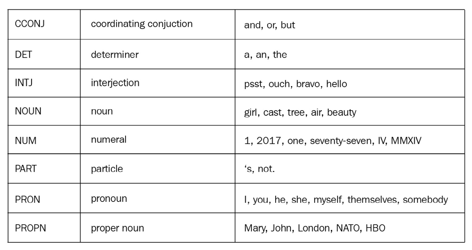
Figure 3.2 – Fine-grained English tags and universal tag mappings

Don't worry if you haven't worked with POS tags before, as you'll become familiar by practicing with the help of our examples. We'll always include explanations of the tags that we use. You can also call spacy.explain() on the tags. We usually call spacy.explain() in two ways, either directly on the tag name string or with token.tag_, as illustrated in the following code snippet:

spacy.explain("NNS)

'noun, plural'

doc = nlp("I saw flowers.")

token = doc[2]

token.text, token.tag_, spacy.explain(token.tag_)

('flowers', 'NNS', 'noun, plural')

If you want to know more about POS, you can read more about it at two excellent resources: Part of Speech at http://partofspeech.org/, and the Eight Parts of Speech at http://www.butte.edu/departments/cas/tipsheets/grammar/parts_of_speech.html.

As you can see, POS tagging offers a very basic syntactic understanding of the sentence. POS tags are used in NLU extensively; we frequently want to find the verbs and the nouns in a sentence and better disambiguate some words for their meanings (more on this subject soon).

Each word is tagged by a POS tag depending on its context—the other surrounding words and their POS tags. POS taggers are sequential statistical models, which means that a tag of a word depends on the word-neighbor tokens, their tags, and the word itself. POS tagging has always been done in different forms. Sequence-to-sequence learning (Seq2seq) started with Hidden Markov Models (HMMs) in the early days and evolved to neural network models—typically, long short-term memory (LSTM) variations (spaCy also uses an LSTM variation). You can witness the evolution of state-of-art POS tagging on the ACL website (https://aclweb.org/aclwiki/POS_Tagging_(State_of_the_art)).

It's time for some code now. Again, spaCy offers universal POS tags via the token.pos (int) and token.pos_ (unicode) features. The fine-grained POS tags are available via the token.tag (int) and token.tag_ (unicode) features. Let's learn more about tags that you'll come across most, through some examples. The following example includes examples of noun, proper noun, pronoun, and verb tags:

import spacy

nlp = spacy.load("en_core_web_md")

doc = nlp("Alicia and me went to the school by bus.")

for token in doc:

    token.text, token.pos_, token.tag_,

    spacy.explain(token.pos_), spacy.explain(token.tag_)

...

('Alicia', 'PROPN', 'NNP', 'proper noun', 'noun, proper singular')

('and', 'CCONJ', 'CC', 'coordinating conjunction', 'conjunction, coordinating')

('me', 'PRON', 'PRP', 'pronoun', 'pronoun, personal')

('went', 'VERB', 'VBD', 'verb', 'verb, past tense')

('to', 'ADP', 'IN', 'adposition', 'conjunction, subordinating or preposition')

('school', 'NOUN', 'NN', 'noun', 'noun, singular or mass')

('with', 'ADP', 'IN', 'adposition', 'conjunction, subordinating or preposition')

('bus', 'NOUN', 'NN', 'noun', 'noun, singular or mass')

('.', 'PUNCT', '.', 'punctuation', 'punctuation mark, sentence closer')

We iterated over the tokens and printed the tokens' text, universal tag, and fine-grained tag, together with the explanations, which are outlined here:

• Alicia is a proper noun, as expected, and NNP is a tag for proper nouns.
• me is a pronoun and bus is a noun. NN is a tag for singular nouns and PRP is a personal pronoun tag.
• Verb tags start with V. Here, VBD is a tag for went, which is a past-tense verb.

Now, consider the following sentence:

doc = nlp("My friend will fly to New York fast and she is staying there for 3 days.")

for token in doc:

    token.text, token.pos_, token.tag_,

    spacy.explain(token.pos_), spacy.explain(token.tag_)

…

('My', 'DET', 'PRP$', 'determiner', 'pronoun, possessive')

('friend', 'NOUN', 'NN', 'noun', 'noun, singular or mass')

('will', 'VERB', 'MD', 'verb', 'verb, modal auxiliary')

('fly', 'VERB', 'VB', 'verb', 'verb, base form')

('to', 'ADP', 'IN', 'adposition', 'conjunction, subordinating or preposition')

('New', 'PROPN', 'NNP', 'proper noun', 'noun, proper singular')

('York', 'PROPN', 'NNP', 'proper noun', 'noun, proper singular')

('fast', 'ADV', 'RB', 'adverb', 'adverb')

('and', 'CCONJ', 'CC', 'coordinating conjunction', 'conjunction, coordinating')

('she', 'PRON', 'PRP', 'pronoun', 'pronoun, personal')

('is', 'AUX', 'VBZ', 'auxiliary', 'verb, 3rd person singular present')

('staying', 'VERB', 'VBG', 'verb', 'verb, gerund or present participle')

('there', 'ADV', 'RB', 'adverb', 'adverb')

('for', 'ADP', 'IN', 'adposition', 'conjunction, subordinating or preposition')

('3', 'NUM', 'CD', 'numeral', 'cardinal number')

('days', 'NOUN', 'NNS', 'noun', 'noun, plural')

('.', 'PUNCT', '.', 'punctuation', 'punctuation mark, sentence closer')

Let's start with the verbs. As we pointed out in the first example, verb tags start with V. Here, there are three verbs, as follows:

• fly: a base form
• staying: an -ing form
• is: an auxiliary verb

The corresponding tags are VB, VBG, and VBZ.

Another detail is both New and York are tagged as proper nouns. If a proper noun consists of multiple tokens, then all the tokens admit the tag NNP. My is a possessive pronoun and is tagged as PRP$, in contrast to the preceding personal pronoun me and its tag PRP.

Let's continue with a word that can be a verb or noun, depending on the context: ship. In the following sentence, ship is used as a verb:

doc = nlp("I will ship the package tomorrow.")

for token in doc:

    token.text, token.tag_, spacy.explain(token.tag_)

...

('I', 'PRP', 'pronoun, personal')

('will', 'MD', 'verb, modal auxiliary')

('ship', 'VB', 'verb, base form')

('the', 'DT', 'determiner')

('package', 'NN', 'noun, singular or mass')

('tomorrow', 'NN', 'noun, singular or mass')

('.', '.', 'punctuation mark, sentence closer')

Here, ship is tagged as a verb, as we expected. Our next sentence also contains the word ship, but as a noun. Now, can the spaCy tagger tag it correctly? Have a look at the following code snippet to find out:

doc = nlp("I saw a red ship.")

for token in doc:

...  token.text, token.tag_, spacy.explain(token.tag_)

...

('I', 'PRP', 'pronoun, personal')

('saw', 'VBD', 'verb, past tense')

('a', 'DT', 'determiner')

('red', 'JJ', 'adjective')

('ship', 'NN', 'noun, singular or mass')

('.', '.', 'punctuation mark, sentence closer')

Et voilà! This time, the word ship is now tagged as a noun, as we wanted to see. The tagger looked at the surrounding words; here, ship is used with a determiner and an adjective, and spaCy deduced that it should be a noun.

How about this tricky sentence:

doc = nlp("My cat will fish for a fish tomorrow in a fishy way.")

for token in doc:

    token.text, token.pos_, token.tag_,

    spacy.explain(token.pos_), spacy.explain(token.tag_)

…

('My', 'DET', 'PRP$', 'determiner', 'pronoun, possessive')

('cat', 'NOUN', 'NN', 'noun', 'noun, singular or mass')

('will', 'VERB', 'MD', 'verb', 'verb, modal auxiliary')

('fish', 'VERB', 'VB', 'verb', 'verb, base form')

('for', 'ADP', 'IN', 'adposition', 'conjunction, subordinating or preposition')

('a', 'DET', 'DT', 'determiner', 'determiner')

('fish', 'NOUN', 'NN', 'noun', 'noun, singular or mass')

('tomorrow', 'NOUN', 'NN', 'noun', 'noun, singular or mass')

('in', 'ADP', 'IN', 'adposition', 'conjunction, subordinating or preposition')

('a', 'DET', 'DT', 'determiner', 'determiner')

('fishy', 'ADJ', 'JJ', 'adjective', 'adjective')

('way', 'NOUN', 'NN', 'noun', 'noun, singular or mass')

('.', 'PUNCT', '.', 'punctuation', 'punctuation mark, sentence closer')

We wanted to fool the tagger with the different usages of the word fish, but the tagger is intelligent enough to distinguish the verb fish, the noun fish, and the adjective fishy. Here's how it did it:

• Firstly, fish comes right after the modal verb will, so the tagger recognized it as a verb.
• Secondly, fish serves as the object of the sentence and is qualified by a determiner; the tag is most probably a noun.
• Finally, fishy ends in y and comes before a noun in the sentence, so it's clearly an adjective.

The spaCy tagger made a very smooth job here of predicting a tricky sentence. After examples of very accurate tagging, only one question is left in our minds: Why do we need the POS tags?

What is the importance of POS tags in NLU, and why do we need to distinguish the class of the words anyway? The answer is simple: many applications need to know the word type for better accuracy. Consider machine translation systems for an example of this: the words for fish (V) and fish (N) correspond to different words in Spanish, as illustrated in the following code snippet:

I will fish/VB tomorrow.  ->  Pescaré/V mañana.

I eat fish/NN.  -> Como pescado/N.

Syntactic information can be used in many NLU tasks, and playing some POS tricks can help your NLU code a lot. Let's continue with a traditional problem: word-sense disambiguation (WSD), and how to tackle it with the help of the spaCy tagger.

WSD

WSD is a classical NLU problem of deciding in which sense a particular word is used in a sentence. A word can have many senses—for instance, consider the word bass. Here are some senses we can think of:

• Bass—seabass, fish (noun (N))
• Bass—lowest male voice (N)
• Bass—male singer with lowest voice range (N)

Determining the sense of the word can be crucial in search engines, machine translation, and question-answering systems. For the preceding example, bass, a POS tagger is unfortunately not much of help as the tagger labels all senses with a noun tag. We need more than a POS tagger. How about the word beat? Let's have a look at this here:

• Beat—to strike violently (verb (V))
• Beat—to defeat someone else in a game or a competition (V)
• Beat—rhythm in music or poetry (N)
• Beat—bird wing movement (N)
• Beat—completely exhausted (adjective (ADJ))

Here, POS tagging can help a lot indeed. The ADJ tag determines the word sense definitely; if the word beat is tagged as ADJ, it identifies the sense completely exhausted. This is not true for the V and N tags here; if the word beat is labeled with a V tag, its sense can be to strike violently or to defeat someone else. WSD is an open problem, and many complicated statistical models are proposed. However, if you need a quick prototype, you can tackle this problem in some cases (such as in the preceding example) with the help of the spaCy tagger.

Verb tense and aspect in NLU applications

In the previous chapter, we used the example of the travel agency application where we got the base forms (which are freed from verb tense and aspect) of the verbs by using lemmatization. In this subsection, we'll focus on how to use the verb tense and aspect information that we lost during the lemmatization process.

Verb tense and aspect are maybe the most interesting information that verbs provide us, telling us when the action happened in time and if the action of the verb is finished or ongoing. Tense and aspect together indicate a verb's reference to the current time. English has three basic tenses: past, present, and future. A tense is accompanied by either simple, progressive/continuous, or perfect aspects. For instance, in the sentence I'm eating, the action eat happens in the present and is ongoing, hence we describe this verb as present progressive/continuous.

So far, so good. So, how do we use this information in our travel agency NLU, then? Consider the following customer sentences that can be directed to our NLU application:

I flew to Rome.

I have flown to Rome.

I'm flying to Rome.

I need to fly to Rome.

I will fly to Rome.

In all the sentences, the action is to fly: however, only some sentences state intent to make a ticket booking. Let's imagine these sentences with a surrounding context, as follows:

I flew to Rome 3 days ago. I still didn't get the bill, please send it ASAP.

I have flown to Rome this morning and forgot my laptop on the airplane. Can you please connect me to lost and found?

I'm flying to Rome next week. Can you check flight availability?

I need to fly to Rome. Can you check flights on next Tuesday?

I will fly to Rome next week. Can you check the flights?   

At a quick glance, past and perfect forms of the verb fly don't indicate a booking intent at all. Rather, they direct to either a customer complaint or customer service issues. The infinitive and present progressive forms, on the other hand, point to booking intent. Let's tag and lemmatize the verbs with the following code segment:

sent1 = "I flew to Rome".

sent2 = "I'm flying to Rome."

sent3 = "I will fly to Rome."

doc1 = nlp(sent1)

doc2 = nlp(sent2)

doc3 = nlp(sent3)

for doc in [doc1, doc2, doc3]

    print([(w.text, w.lemma_) for w in doc if w.tag_== 'VBG' or w.tag_== 'VB'])

...

[]

[('flying', 'fly')]

[('fly', 'fly')]

We iterated three doc objects one by one, and for each sentence we checked if the fine-grained tag of the token is VBG (a verb in present progressive form) or VB (a verb in base/infinitive form). Basically, we filtered out the present progressive and infinitive verbs. You can think of this process as a semantic representation of the verb in the form of (word form, lemma, tag) as illustrated in the following code snippet:

flying: (fly, VBG)

We have covered one semantic and one morphological task—WSD and tense/aspect of verbs. We'll continue with a tricky subject: how to make the best of some special tags—namely, number, symbol, and punctuation tags.

Understanding number, symbol, and punctuation tags

If you look at the English POS, you will notice the NUM, SYM, and PUNCT tags. These are the tags for numbers, symbols, and punctuation, respectively. These categories are divided into fine-grained categories: $, SYM, '', -LRB-, and -RRB-. These are shown in the following screenshot:

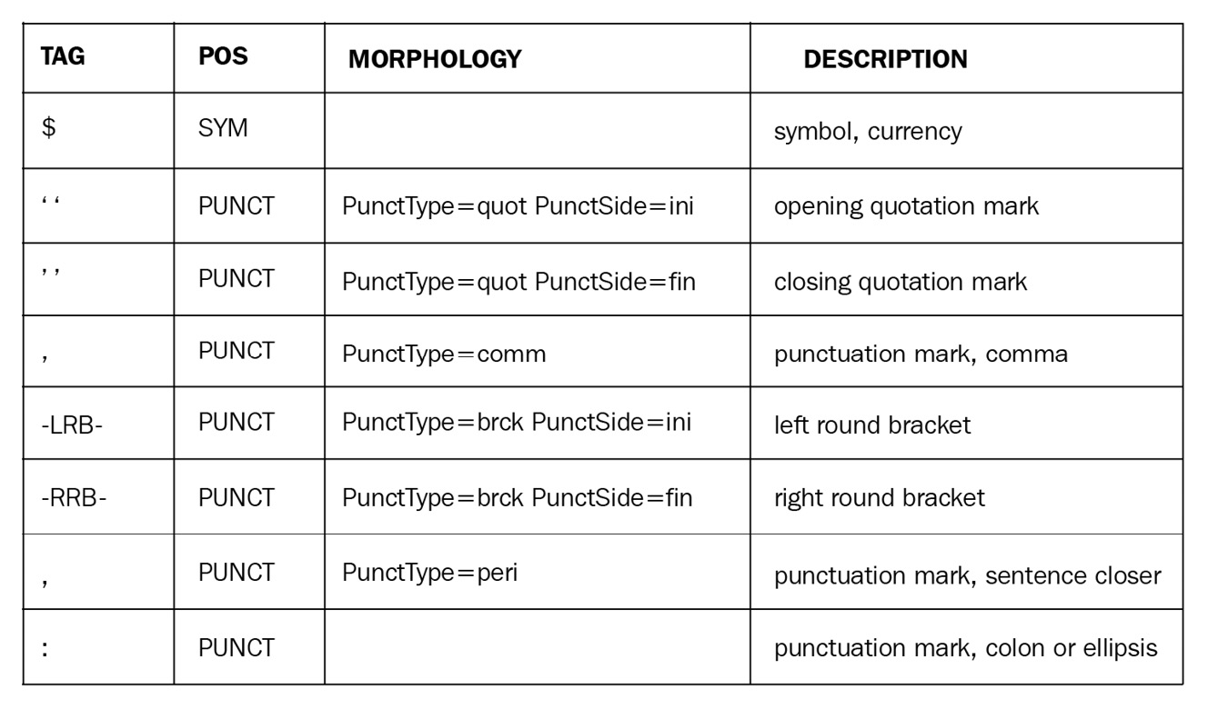
Figure 3.3 – spaCy punctuation tags, general and fine-grained

Let's tag some example sentences that contain numbers and symbols, as follows:

doc = nlp("He earned $5.5 million in 2020 and paid %35 tax.")

for token in doc:

    token.text, token.tag_, spacy.explain(token.tag_)

...

('He', 'PRP', 'pronoun, personal')

('earned', 'VBD', 'verb, past tense')

('$', '$', 'symbol, currency')

('5.5', 'CD', 'cardinal number')

('million', 'CD', 'cardinal number')

('in', 'IN', 'conjunction, subordinating or preposition')

('2020', 'CD', 'cardinal number')

('and', 'CC', 'conjunction, coordinating')

('paid', 'VBD', 'verb, past tense')

('35', 'CD', 'cardinal number')

('percent', 'NN', 'noun, singular or mass')

('tax', 'NN', 'noun, singular or mass')

('.', '.', 'punctuation mark, sentence closer')

We again iterated over the tokens and printed the fine-grained tags. The tagger was able to distinguish symbols, punctuation marks, and numbers. Even the word million is recognized as a number too!

Now, what to do with symbol tags? Currency symbols and numbers offer a way to systematically extract descriptions of money and are very handy in financial text such as financial reports. We'll see how to extract money entities in Chapter 4, Rule-Based Matching.

That's it—you made it to the end of this exhaustive section! There's a lot to unpack and digest, but we assure you that you made a great investment for your industrial NLP work. We'll now continue with another syntactic concept—dependency parsing.

Introduction to dependency parsing

If you are already familiar with spaCy, you must have come across the spaCy dependency parser. Though many developers see dependency parser on the spaCy documentation, they're shy about using it or don't know how to use this feature to the fullest. In this part, you'll explore a systematic way of representing a sentence syntactically. Let's start with what dependency parsing actually is.

What is dependency parsing?

In the previous section, we focused on POS tags—syntactic categories of words. Though POS tags provide information about neighbor words' tags as well, they do not give away any relations between words that are not neighbors in the given sentence.

In this section, we'll focus on dependency parsing—a more structured way of exploring the sentence syntax. As the name suggests, dependency parsing is related to analyzing sentence structures via dependencies between the tokens. A dependency parser tags syntactic relations between tokens of the sentence and connects syntactically related pairs of tokens. A dependency or a dependency relation is a directed link between two tokens.

The result of the dependency parsing is always a tree, as illustrated in the following screenshot:

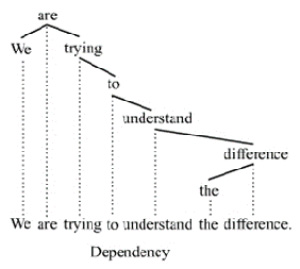
Figure 3.4 – An example of a dependency tree (taken from Wikipedia)

If you're not familiar with a tree data structure, you can learn more about it at this excellent Computer Science resource:

https://www.cs.cmu.edu/~clo/www/CMU/DataStructures/Lessons/lesson4_1.htm

Dependency relations

What is the use of dependency relations, then? Quite a number of statistical methods in NLP revolve around vector representations of words and treat a sentence as a sequence of words. As you can see in Figure 3.4, a sentence is more than a sequence of tokens—it has a structure; every word in a sentence has a well-defined role, such as verb, subject, object, and so on; hence, sentences definitely have a structure. This structure is used extensively in chatbots, question answering, and machine translation.

The most useful application that first comes to mind is determining the sentence object and subject. Again, let's go back to our travel agency application. Imagine a customer is complaining about the service. Compare the two sentences, I forwarded you the email and You forwarded me the email; if we eliminate the stopwords I, you, me, and the, this is what remains:

I forwarded you the email. -> forwarded email

You forwarded me the email. -> forwarded email

Though the remaining parts of the sentences are identical, sentences have very different meanings and require different answers. In the first sentence, the sentence subject is I (then, the answer most probably will start with you) and the second sentence's subject is you (which will end up in an I answer).

Obviously, the dependency parser helps us to go deeper into the sentence syntax and semantics. Let's explore more, starting from the dependency relations.

Syntactic relations

spaCy assigns each token a dependency label, just as with other linguistic features such as a lemma or a POS tag. spaCy shows dependency relations with directed arcs. The following screenshot shows an example of a dependency relation between a noun and the adjective that qualifies the noun:

Figure 3.5 – Dependency relation between a noun and its adjective

A dependency label describes the type of syntactic relation between two tokens as follows: one of the tokens is the syntactic parent (called the HEAD) and the other is its dependent (called the CHILD). In the preceding example, flower is the head and blue is its dependent/child.

The dependency label is assigned to the child. Token objects have dep (int) and dep_ (unicode) properties that hold the dependency label, as illustrated in the following code snippet:

doc = nlp("blue flower")

for token in doc:

    token.text, token.dep_

…

('blue', 'amod')

('flower', 'ROOT')

In this example, we iterated over the tokens and printed their text and dependency label. Let's go over what happened bit by bit, as follows:

• blue admitted the amod label. amod is the dependency label for an adjective-noun relation. For more examples of the amod relation, please refer to Figure 3.7.
• flower is the ROOT. ROOT is a special label in the dependency tree; it is assigned to the main verb of a sentence. If we're processing a phrase (not a full sentence), the ROOT label is assigned to the root of the phrase, which is the head noun of the phrase. In the blue flower phrase, the head noun, flower, is the root of the phrase.
• Each sentence/phrase has exactly one root, and it's the root of the parse tree (remember, the dependency parsing result is a tree).
• Tree nodes can have more than one child, but each node can only have one parent (due to tree restrictions, and trees containing no cycles). In other words, every token has exactly one head, but a parent can have several children. This is the reason why the dependency label is assigned to the dependent node.

Here is a full list of spaCy's English dependency labels:

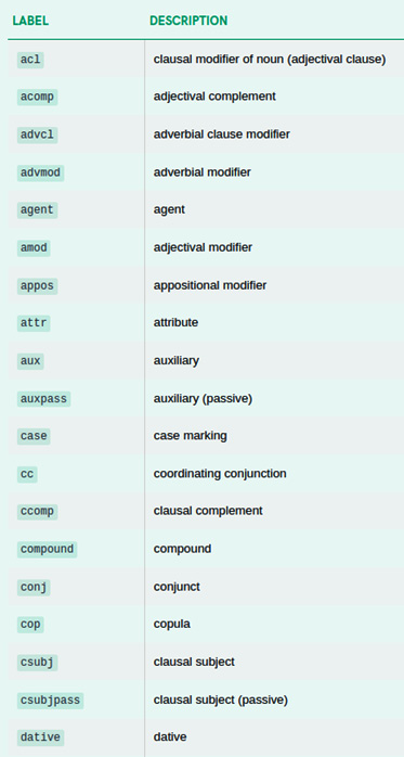
Figure 3.6 – List of spaCy English dependency labels

That's a long list! No worries—you don't need to memorize every list item. Let's first see a list of the most common and useful labels, then we'll see how exactly they link tokens to each other. Here's the list first:

• amod: Adjectival modifier
• aux: Auxiliary
• compound: Compound
• dative: Dative object
• det: Determiner
• dobj: Direct object
• nsubj: Nominal subject
• nsubjpass: Nominal subject, passive
• nummod: Numeric modifier
• poss: Possessive modifier
• root: The root

Let's see examples of how the aforementioned labels are used and what relation they express. amod is adjectival modifier. As understood from the name, this relation modifies the noun (or pronoun). In the following screenshot, we see white modifies sheep:

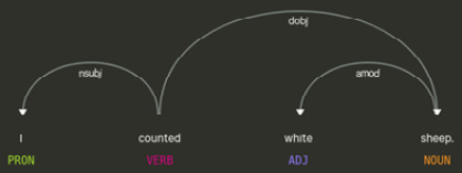
Figure 3.7 – amod relation

aux is what you might guess: it's the dependency relation between an auxiliary verb and its main verb; the dependent is an auxiliary verb, and the head is the main verb. In the following screenshot, we see that has is the auxiliary verb of the main verb gone:

Figure 3.8 – aux relation

compound is used for the noun compounds; the second noun is modified by the first noun. In the following screenshot, phone book is a noun compound and the phone noun modifies the book noun:

Figure 3.9 – Compound relation between phone and book

The det relation links a determiner (the dependent) to the noun it qualifies (its head). In the following screenshot, the is the determiner of the noun girl in this sentence:

Figure 3.10 – det relation

Next, we look into two object relations, dative and dobj. The dobj relation is between the verb and its direct object. A sentence can have more than one object (such as in the following example); a direct object is the object that the verb acts upon, and the others are called indirect objects.

A direct object is generally marked with accusative case. A dative relation points to a dative object, which receives an indirect action from the verb. In the sentence shown in the following screenshot, the indirect object is me and the direct object is book:

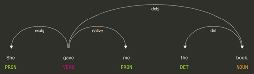
Figure 3.11 – The direct and indirect objects of the sentence

nsubj and nsubjposs are two relations that are related to the nominal sentence subject. The subject of the sentence is the one that committed the action. A passive subject is still the subject, but we mark it with nsubjposs. In the following screenshot, Mary is the nominal subject of the first sentence:

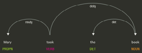
Figure 3.12 – nsubj relation

you is the passive nominal subject of the sentence in the following screenshot:

Figure 3.13 – nsubjpass relation

We have now covered sentence subject and object relations. Now, we'll discover two modifier relations; one is the nummod numeric modifier and the other is the poss possessive modifier. A numeric modifier modifies the meaning of the head noun by a number/quantity. In the sentence shown in the following screenshot, nummod is easy to spot; it's between 3 and books:

Figure 3.14 – nummod relation

A possessive modifier happens either between a possessive pronoun and a noun or a possessive 's and a noun. In the sentence shown in the following screenshot, my is a possessive marker on the noun book:

Figure 3.15 – poss relation between "my" and "book"

Last, but not least, is the root label, which is not a real relation but is a marker for the sentence verb. A root word has no real parent in the syntactic tree; the root is the main verb of the sentence. In the preceding sentences, took and given are the corresponding roots. The main verbs of both sentences are the auxiliary verbs is and are. Notice that the root node has no incoming arc—that is, no parent.

These are the most useful labels for our NLU purposes. You definitely don't need to memorize all the labels, as you'll become familiar as you practice in the next pages. Also, you can ask spaCy about a label any time you need, via spacy.explain(). The code to do this is shown in the following snippet:

spacy.explain("nsubj")

'nominal subject'

doc = nlp("I own a ginger cat.")

token = doc[4]

token.text, token.dep_, spacy.explain(token.dep_)

('cat', 'dobj', 'direct object')

Take a deep breath, since there is a lot to digest! Let's practice how we can make use of dependency labels.

Again, token.dep_ includes the dependency label of the dependent token. The token.head property points to the head/parent token. Only the root token does not have a parent; spaCy points to the token itself in this case. Let's bisect the example sentence from Figure 3.7, as follows:

doc = nlp("I counted white sheep.")

for token in doc:

    token.text, token.pos_, token.dep_

...

('I', 'PRP', 'nsubj')

('counted', 'VBD', 'ROOT')

('white', 'JJ', 'amod')

('sheep', 'NNS', 'dobj')

('.', '.', 'punct')

We iterated over the tokens and printed the fine-grained POS tag and the dependency label. counted is the main verb of the sentence and is labeled by the label ROOT. Now, I is the subject of the sentence, and sheep is the direct object. white is an adjective and modifies the noun sheep, hence its label is amod. We go one level deeper and print the token heads this time, as follows:

doc = nlp(“I counted white sheep.”)

for token in doc:

      token.text, token.tag_, token.dep_, token.head

...

('I', 'PRP', 'nsubj', counted)

('counted', 'VBD', 'ROOT', counted)

('white', 'JJ', 'amod', sheep)

('sheep', 'NNS', 'dobj', counted)

('.', '.', 'punct', counted)

The visualization is as follows:

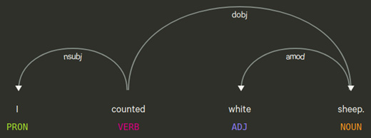
Figure 3.16 – An example parse of a simple sentence

When the token.head property is also involved, it's a good idea to follow the code and the visual at the same time. Let's go step by step in order to understand how the visual and the code match:

1. We start reading the parse tree from the root. It's the main verb: counted.
2. Next, we follow its arc on the left toward the pronoun I, which is the nominal subject of the sentence and is labeled by the label nsubj.
3. Now, return back to the root, counted. This time, we navigate to the right. Follow the dobj arc to reach the noun sheep. sheep is modified by the adjective white with an amod relation, hence the direct object of this sentence is white sheep.

Even such a simple, flat sentence has a dependency parse tree that's fancy to read, right? Don't rush—you'll get used to it by practicing. Let's examine the dependency tree of a longer and more complicated sentence, as follows:

doc = nlp("We are trying to understand the difference.")

for token in doc:

    token.text, token.tag_, token.dep_, token.head

...

('We', 'PRP', 'nsubj', trying)

('are', 'VBP', 'aux', trying)

('trying', 'VBG', 'ROOT', trying)

('to', 'TO', 'aux', understand)

('understand', 'VB', 'xcomp', trying)

('the', 'DT', 'det', difference)

('difference', 'NN', 'dobj', understand)

('.', '.', 'punct', trying)

Now, this time things look a bit different, as we'll see in Figure 3.17. We locate the main verb and the root trying (it has no incoming arcs). The left side of the word trying looks manageable, but the right side has a chain of arcs. Let's start with the left side. The pronoun we is labeled by nsubj, hence this is the nominal subject of the sentence. The other left arc, labeled aux, points to the trying dependent are, which is the auxiliary verb of the main verb trying.

So far, so good. Now, what is happening on the right side? trying is attached to the second verb understand via an xcomp relation. The xcomp (or open complement) relation of a verb is a clause without its own subject. Here, the to understand the difference clause has no subject, so it's an open complement. We follow the dobj arc from the second verb, understand, and land on the noun, difference, which is the direct object of the to understand the difference clause, and this is the result:

Figure 3.17 – A complicated parsing example

This was an in-depth analysis for this example sentence, which indeed does not look that complicated. Next, we process a sentence with a subsentence that owns its own nominal subject, as follows:

doc = nlp("Queen Katherine, who was the mother of Mary Tudor, died at 1536.")

for token in doc:

    token.text, token.tag_, token.dep_, token.head

...

('Queen', 'NNP', 'compound', Katherine)

('Katherine', 'NNP', 'nsubj', died)

(',', ',', 'punct', Katherine)

('who', 'WP', 'nsubj', was)

('was', 'VBD', 'relcl', Katherine)

('the', 'DT', 'det', mother)

('mother', 'NN', 'attr', was)

('of', 'IN', 'prep', mother)

('Mary', 'NNP', 'compound', Tudor)

('Tudor', 'NNP', 'pobj', of)

(',', ',', 'punct', Katherine)

('died', 'VBD', 'ROOT', died)

('at', 'IN', 'prep', died)

('1536', 'CD', 'pobj', at)

In order to make the visuals big enough, I have split the visualization into two parts. First, let's find the root. The root lies in the right part. died is the main sentence of the verb and the root (again, it has no incoming arcs). The rest of the right side contains nothing tricky.

On the other hand, the left side has some interesting stuff—actually, a relative clause. Let's bisect the relative clause structure:

• We start with the proper noun Katherine, which is attached to died with a nsubj relation, hence the subject of the sentence.
• We see a compound arc leaving Katherine toward the proper noun, Queen. Here, Queen is a title, so the relationship with Katherine is compound. The same relationship exists between Mary and Tudor on the right side, and the last names and first names are also tied with the compound relation.

It's time to bisect the relative clause, who was the mother of Mary Tudor, as follows:

• First of all, it is Katherine who is mentioned in the relative clause, so we see a relcl (relative clause) arc from Katherine to was of the relative clause.
• who is the nominal subject of the clause and is linked to was via an nsubj relation. As you see in the following screenshot, the dependency tree is different from the previous example sentence, whose clause didn't own a nominal subject:

Figure 3.18 – A dependency tree with a relative clause, the left part

Figure 3.19 – Same sentence, the right part

It's perfectly normal if you feel that you won't be able to keep all the relations in your mind. No worries—always find the root/main verb of the sentence, then follow the arcs from the root and go deeper, just as we did previously. You can always have a look at the spaCy documentation (https://spacy.io/api/annotation#dependency-parsing) to see what the relation type means. Take your time until you warm up to the concept and the details.

That was exhaustive! Dear reader—as we said before, please take your time to digest and practice on example sentences. The displaCy online demo is a great tool, so don't be shy to try your own example sentences and see the parsing results. It's perfectly normal for you to find this section heavy. However, this section is a solid foundation for general linguistics, and also for the information extraction and pattern-matching exercises in Chapter 4, Rule-Based Matching. You will become even more comfortable after going through a case study in Chapter 6, Putting Everything Together: Semantic Parsing with spaCy. Give yourself time to digest dependency parsing with examples throughout the book.

What comes after the dependency parser? Without any doubt, you must have heard NER frequently mentioned in the NLU world. Let's look into this very important NLU concept.

Introducing NER

We opened this chapter with a tagger, and we'll see another very handy tagger—the NER tagger of spaCy. As NER's name suggests, we are interested in finding named entities.

What is a named entity? A named entity is a real-world object that we can refer to by a proper name or a quantity of interest. It can be a person, a place (city, country, landmark, famous building), an organization, a company, a product, dates, times, percentages, monetary amounts, a drug, or a disease name. Some examples are Alicia Keys, Paris, France, Brandenburg Gate, WHO, Google, Porsche Cayenne, and so on.

A named entity always points to a specific object, and that object is distinguishable via the corresponding named entity. For instance, if we tag the sentence Paris is the capital of France, we parse Paris and France as named entities, but not the word capital. The reason is that capital does not point to a specific object; it's a general name for many objects.

NER categorization is a bit different from POS categorization. Here, the number of categories is as high as we want. The most common categories are person, location, and organization and are supported by almost every usable NER tagger. In the following screenshot, we see the corresponding tags:

Figure 3.20 – Most common entity types

spaCy supports a wide range of entity types. Which ones you use depends on your corpus. If you process financial text, you most probably use MONEY and PERCENTAGE more often than WORK_OF_ART.

Here is a list of the entity types supported by spaCy:

Figure 3.21 – Full list of entity types supported by spaCy

Just as with the POS tagger statistical models, NER models are also sequential models. The very first modern NER tagger model is a conditional random field (CRF). CRFs are sequence classifiers used for structured prediction problems such as labeling and parsing. If you want to learn more about the CRF implementation details, you can read more at this resource: https://homepages.inf.ed.ac.uk/csutton/publications/crftutv2.pdf. The current state-of-the-art NER tagging is achieved by neural network models, usually LSTM or LSTM+CRF architectures.

Named entities in a doc are available via the doc.ents property. doc.ents is a list of Span objects, as illustrated in the following code snippet:

doc = nlp("The president Donald Trump visited France.")

doc.ents

(Donald Trump, France)

type(doc.ents[1])

<class 'spacy.tokens.span.Span'>

spaCy also tags each token with the entity type. The type of the named entity is available via token.ent_type (int) and token.ent_type_ (unicode). If the token is not a named entity, then token.ent_type_ is just an empty string.

Just as for POS tags and dependency labels, we can call spacy.explain() on the tag string or on the token.ent_type_, as follows:

spacy.explain("ORG")

'Companies, agencies, institutions, etc.

doc = nlp("He worked for NASA.")

token = doc[3]

token.ent_type_, spacy.explain(token.ent_type_)

('ORG', 'Companies, agencies, institutions, etc.')

Let's go over some examples to see the spaCy NER tagger in action, as follows:

doc = nlp("Albert Einstein was born in Ulm on 1879. He studied electronical engineering at ETH Zurich.")

doc.ents

(Albert Einstein, Ulm, 1879, ETH Zurich)

for token in doc:

    token.text, token.ent_type_,

    spacy.explain(token.ent_type_)

...

('Albert', 'PERSON', 'People, including fictional')

('Einstein', 'PERSON', 'People, including fictional')

('was', '', None)

('born', '', None)

('in', '', None)

('Ulm', 'GPE', 'Countries, cities, states')

('on', '', None)

('1879', 'DATE', 'Absolute or relative dates or periods')

('.', '', None)

('He', '', None)

('studied', '', None)

('electronical', '', None)

('engineering', '', None)

('at', '', None)

('ETH', 'ORG', 'Companies, agencies, institutions, etc.')

('Zurich', 'ORG', 'Companies, agencies, institutions, etc.')

('.', '', None)

We iterated over the tokens one by one and printed the token and its entity type. If the token is not tagged as an entity, then token.ent_type_ is just an empty string, hence there is no explanation from spacy.explain(). For the tokens that are part of a NE, an appropriate tag is returned. In the preceding sentences, Albert Einstein, Ulm, 1879, and ETH Zurich are correctly tagged as PERSON, GPE, DATE, and ORG, respectively.

Let's see a longer and more complicated sentence with a non-English entity and look at how spaCy tagged it, as follows:

doc = nlp("Jean-Michel Basquiat was an American artist of Haitian and Puerto Rican descent who gained fame with his graffiti and street art work")

doc.ents

(Jean-Michel Basquiat, American, Haitian, Puerto Rican)

for ent in doc.ents:

    ent, ent.label_, spacy.explain(ent.label_)

...

(Jean-Michel Basquiat, 'PERSON', 'People, including fictional')

(American, 'NORP', 'Nationalities or religious or political groups')

(Haitian, 'NORP', 'Nationalities or religious or political groups')

(Puerto Rican, 'NORP', 'Nationalities or religious or political groups')

Looks good! The spaCy tagger picked up a person entity with a - smoothly. Overall, the tagger works quite well for different entity types, as we saw throughout the examples.

After tagging tokens with different syntactical features, we sometimes want to merge/split entities into fewer/more tokens. In the next section, we will see how merging and splitting is done. Before that, we will see a real-world application of NER tagging.

A real-world example

NER is a popular and frequently used pipeline component of spaCy. NER is one of the key components of understanding the text topic, as named entities usually belong to a semantic category. For instance, President Trump invokes the politics subject in our minds, whereas Leonardo DiCaprio is more about movies. If you want to go deeper into resolving the text meaning and understanding who made what, you also need named entities.

This real-world example includes processing a New York Times article. Let's go ahead and download the article first by running the following code:

from bs4 import BeautifulSoup

import requests

import spacy

def url_text(url_string):

    res = requests.get(url)

    html = res.text

    soup = BeautifulSoup(html, 'html5lib')

    for script in soup(["script", "style", 'aside']):

        script.extract()

    text = soup.get_text()

    return " ".join(text.split())

ny_art = url_text("https://www.nytimes.com/2021/01/12/opinion/trump-america-allies.html")

nlp = spacy.load("en_core_web_md")

doc = nlp(ny_art)

We downloaded the article Uniform Resource Locator (URL), and then we stripped the article text from the HyperText Markup Language (HTML). BeautifulSoup is a popular Python package for extracting text from HTML and Extensible Markup Language (XML) documents. Then, we created a nlp object, passed the article body to the nlp object, and created a Doc object.

Let's start our analysis of the article by the entity type count, as follows:

len(doc.ents)

136

That's a totally normal number for a news article that includes many entities. Let's go a bit further and group the entity types, as follows:

from collections import Counter

labels = [ent.label_ for ent in doc.ents]

Counter(labels)

Counter({'GPE': 37, 'PERSON': 30, 'NORP': 24, 'ORG': 22, 'DATE': 13, 'CARDINAL': 3, 'FAC': 2, 'LOC': 2, 'EVENT': 1, 'TIME': 1, 'WORK_OF_ART': 1})

The most frequent entity type is GPE, which means a country, city, or state. The second one is PERSON, whereas the third most frequent entity label is NORP, which means a nationality/religious-political group. The next ones are organization, date, and cardinal number-type entities.

Can we summarize the text by looking at the entities or understanding the text topic? To answer this question, let's start by counting the most frequent tokens that occur in the entities, as follows:

items = [ent.text for ent in doc.ents]

Counter(items).most_common(10)

[('America', 12), ('American', 8), ('Biden', 8), ('China', 6), ('Trump', 5), ('Capitol', 4), ('the United States', 3), ('Washington', 3), ('Europeans', 3), ('Americans', 3)]

Looks like a semantic group! Obviously, this article is about American politics, and possibly how America interacts with the rest of the world in politics. If we print all the entities of the article, we can see here that this guess is true:

print(doc.ents)

(The New York Times SectionsSEARCHSkip, indexLog inToday, storyOpinionSupported byContinue, LaughingstockLast week's, U.S., U.S., Ivan KrastevMr, Krastev, Jan., 2021 A, Rome, Donald Tramp, Thursday, Andrew Medichini, Associated PressDonald Trump, America, America, Russian, Chinese, Iranian, Jan. 6, Capitol, Ukraine, Georgia, American, American, the United States, Trump, American, Congress, Civil War, 19th-century, German, Otto von Bismarck, the United States of America, America, Capitol, Trump, last hours, American, American, Washington, Washington, Capitol, America, America, Russia, at least 10, Four years, Trump, Joe Biden, two, American, China, Biden, America, Trump, Recep Tayyip Erdogan, Turkey, Jair Bolsonaro, Brazil, Washington, Russia, China, Biden, Gianpaolo Baiocchi, H. Jacob Carlson, Social Housing Development Authority, Ezra Klein, Biden, Mark Bittman, Biden, Gail Collins, Joe Biden, Jake Sullivan, Biden, trans-Atlantic, China, Just a week ago, European, Sullivan, Europe, America, China, Biden, Europeans, China, German, Chinese, the European Union's, America, Christophe Ena, the European Council on Foreign Relations, the weeks, American, the day, Biden, Europeans, America, the next 10 years, China, the United States, Germans, Trump, Americans, Congress, America, Bill Clinton, Americans, Biden, the White House, the United States, Americans, Europeans, the past century, America, the days, Capitol, democratic, Europe, American, America, Ivan Krastev, the Center for Liberal Strategies, the Institute for Human Sciences, Vienna, Is It Tomorrow Yet?:, The New York Times Opinion, Facebook, Twitter (@NYTopinion, Instagram, AdvertisementContinue, IndexSite Information Navigation© 2021, The New York Times, GTM, tfAzqo1rYDLgYhmTnSjPqw&gtm_preview)

We made a visualization of the whole article by pasting the text into displaCy Named Entity Visualizer (https://explosion.ai/demos/displacy-ent/). The following screenshot is taken from the demo page that captured a part of the visual:

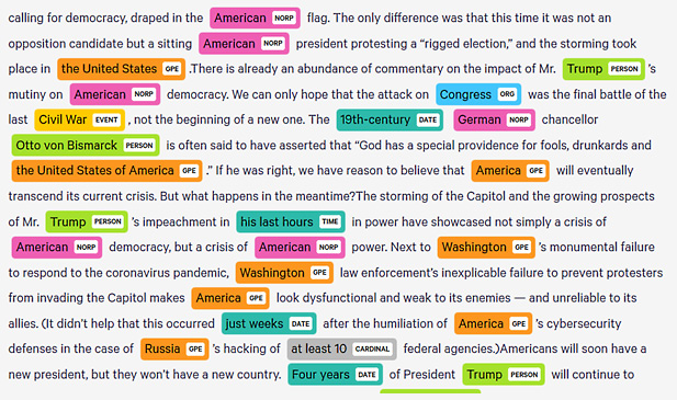
Figure 3.22 – The New York Times article's entities visualized by displaCy

spaCy's NER offers great capabilities for understanding text, as well as presenting good-looking visuals to ourselves, colleagues, and stakeholders.

Merging and splitting tokens

We extracted the name entities in the previous section, but how about if we want to unite or split multiword named entities? And what if the tokenizer performed this not so well on some exotic tokens and you want to split them by hand? In this subsection, we'll cover a very practical remedy for our multiword expressions, multiword named entities, and typos.

doc.retokenize is the correct tool for merging and splitting the spans. Let's see an example of retokenization by merging a multiword named entity, as follows:

doc = nlp("She lived in New Hampshire.")

doc.ents

(New Hampshire,)

[(token.text, token.i) for token in doc]

[('She', 0), ('lived', 1), ('in', 2), ('New', 3), ('Hampshire', 4), ('.', 5)]

len(doc)

6

with doc.retokenize() as retokenizer:

    retokenizer.merge(doc[3:5],

    attrs={"LEMMA": "new hampshire"})

...

[(token.text, token.i) for token in doc]

[('She', 0), ('lived', 1), ('in', 2), ('New Hampshire', 3), ('.', 4)]

len(doc)

5

doc.ents

(New Hampshire,)

[(token.lemma_) for token in doc]

['-PRON-', 'live', 'in', 'new hampshire', '.']

This is what we did in the preceding code:

1. First, we created a doc object from the sample sentence.
2. Then, we printed its entities with doc.ents, and the result was New Hampshire, as expected.
3. In the next line, for each token, we printed token.text with token indices in the sentence (token.i).
4. Also, we examined length of the doc object by calling len on it, and the result was 6 ("." is a token too).

Now, we wanted to merge the tokens of position 3 until 5 (3 is included; 5 is not), so we did the following:

1. First, we called the retokenizer method merge(indices, attrs). attrs is a dictionary of token attributes we want to assign to the new token, such as lemma, pos, tag, ent_type, and so on.
2. In the preceding example, we set the lemma of the new token; otherwise, the lemma would be New only (the starting token's lemma of the span we want to merge).
3. Then, we printed the tokens to see if the operation worked as we wished. When we print the new tokens, we see that the new doc[3] is the New Hampshire token.
4. Also, the doc object is of length 5 now, so we shrank the doc one less token. doc.ents remain the same and the new token's lemma is new hampshire because we set it with attrs.

Looks good, so how about splitting a multiword token into several tokens? In this setting, either there's a typo in the text you want to fix or the custom tokenization is not satisfactory for your specific sentence.

Splitting a span is a bit more complicated than merging a span because of the following reasons:

• We are changing the dependency tree.
• We need to assign new POS tags, dependency labels, and necessary token attributes to the new tokens.
• Basically, we need to think about how to assign linguistic features to the new tokens we created.

Let's see how to deal with the new tokens with an example of how to fix a typo, as follows:

doc = nlp("She lived in NewHampshire")

len(doc)

5

[(token.text, token.lemma_, token.i) for token in doc]

[('She', '-PRON-', 0), ('lived', 'live', 1), ('in', 'in', 2), ('NewHampshire', 'NewHampshire', 3), ('.', '.', 4)]

for token in doc:

    token.text, token.pos_, token.tag_, token.dep_

...

('She', 'PRON', 'PRP', 'nsubj')

('lived', 'VERB', 'VBD', 'ROOT')

('in', 'ADP', 'IN', 'prep')

('NewHampshire', 'PROPN', 'NNP', 'pobj')

('.', 'PUNCT', '.', 'punct')

Here's what the dependency tree looks like before the splitting operation:

Figure 3.23 – Sample sentence's dependency tree before retokenization

Now, we will split the doc[3], NewHampshire, into two tokens: New and Hampshire. We will give fine-grained POS tags and dependency labels to the new tokens via the attrs dictionary. We will also rearrange the dependency tree by passing the new tokens' parents via the heads parameter. While arranging the heads, there are two things to consider, as outlined here:

• Firstly, if you give a relative position (such as (doc[3], 1)) in the following code segment, this means that head of doc[3] will be the +1th position token—that is, doc[4] in the new setup (please see the following visualization ).
• Secondly, if you give an absolute position, it means the position in the original Doc object. In the following code snippet, the second item in the heads list means that the Hampshire token's head is the second token in the original Doc, which is the in token (please refer to Figure 3.23).

After the splitting, we printed the list of new tokens and the linguistic attributes. Also, we examined the new length of the doc object, which is 6 now. You can see the result here:

with doc.retokenize() as retokenizer:

    heads = [(doc[3], 1), doc[2]]

    attrs = {"TAG":["NNP", "NNP"],

              "DEP": ["compound", "pobj"]}

    retokenizer.split(doc[3], ["New", "Hampshire"],

                       heads=heads, attrs=attrs)

...

[(token.text, token.lemma_, token.i) for token in doc]

[('She', '-PRON-', 0), ('lived', 'live', 1), ('in', 'in', 2), ('New', 'New', 3), ('Hampshire', 'Hampshire', 4), ('.', '.', 5)]

for token in doc:

    token.text, token.pos_, token.tag_, token.dep_

...

('She', 'PRON', 'PRP', 'nsubj')

('lived', 'VERB', 'VBD', 'ROOT')

('in', 'ADP', 'IN', 'prep')

('New', 'PROPN', 'NNP', 'pobj')

('Hampshire', 'PROPN', 'NNP', 'compound')

('.', 'PUNCT', '.', 'punct')

len(doc)

6

Here's what the dependency tree looks like after the splitting operation (please compare this with Figure 3.22):

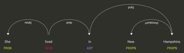
Figure 3.24 – Dependency tree after the splitting operation

You can apply merging and splitting onto any span, not only the named entity spans. The most important part here is to correctly arrange the new dependency tree and the linguistic attributes.

Summary

That was it—you made it to the end of this chapter! It was an exhaustive and long journey for sure, but we have unveiled the real linguistic power of spaCy to the fullest. This chapter gave you details of spaCy's linguistic features and how to use them.

You learned about POS tagging and applications, with many examples. You also learned about an important yet not so well-known and well-used feature of spaCy—the dependency labels. Then, we discovered a famous NLU tool and concept, NER. We saw how to do named entity extraction, again via examples. We finalized this chapter with a very handy tool for merging and splitting the spans that we calculated in the previous sections.

What's next, then? In the next chapter, we will again be discovering a spaCy feature that you'll be using every day in your NLP application code—spaCy's Matcher class. We don't want to give a spoiler on this beautiful subject, so let's go onto our journey together!