
The Coil of Life
12.1 Background
Although the human genome has now been decoded, the focus of investigations on the molecular form and biochemical functions of the gene continues unabated. One question of interest has been the manner in which the long strands of DNA are packed into the tiny confines of a cell. This is a complicated topic, but we can obtain a brief glimpse into some of the mathematical issues it raises.
In terms of the math, this chapter is an exercise in the differential geometry of space curves. The core idea is the linking of two such curves, and in Section 12.4 we sketch a proof, due to Carl Friedrich Gauss, that shows how many times the curves are entwined. This result is not only of interest in itself (and a good use of multivariate calculus), but it also provides some of the background material needed for the introductory and somewhat-intuitive discussion of DNA in Section 12.3. What we do there is to study the possible deformations of this molecule within a cell. The relevant concepts about the link, twist, and writhe of curves is provided in Section 12.2.
12.2 Link, Twist, and Writhe
Without getting into unneeded details, DNA consists of four bases, labeled A, C, G, and T, in which A pairs with T and C with G, each of these hooked together by a weak chemical bond. The pairs form nearly flat molecules that are stacked up like steps on a helical ladder. The edges of the bases are joined to two sugar-phosphate molecular strands that wind around the outside to form a double helix (Figure 12.1a). A simple model of the double helix represents the outer strands as two space curves C1 and C2 that form the bounding edges of a fictional ribbon that makes up a continuous spiral “ladder” (Figure 12.1b).
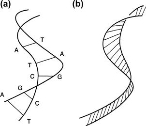
FIGURE 12.1 Schematic of DNA of two sugar-phosphate strands winding about a central backbone of bases (a) and a ribbon model of the DNA in which the edges can, depending on context, represent either two sugar-phosphate strands or one strand connected to the central backbone of bases (b).
The central axis of the ribbon can writhe in space, the two strands forming the boundary of the ribbon can coil about each other, and the whole ribbon can twist about its axis. In Section 12.4 we present an essentially complete proof of a theorem showing that the number of times two closed curves C1 and C2 are linked together is given by the formula
![]() (12.1)
(12.1)
where v is a vector directed from a generic point on C1 to some other position on C2 and T1, T2 are the unit tangent vectors to C1, C2 at these points. The double integral of the triple scalar product is with respect to arc-length parameters s and τ along the two curves.
Some DNA occurs in nature as closed loops, which is the configuration that will be considered here. The two strands defined by curves C1 and C2 link each other as they coil in and above. We now want to discuss twisting and writhing, beginning with the first.
Twisting is essentially a measure of the extent to which C2 spins about C1. It is probably more appropriate in the following to think of C1 as the central backbone of bases in DNA rather than as the other sugar-phosphate strand, at least when talking about twist. But this distinction is sometimes blurred to simplify the discussion.
To be mathematically correct, assume that surfaces defined by the ribbon and its bounding curves are sufficiently smooth that all derivatives exist and are continuous. Let T denote the unit tangent vector to C1 at any point s along this curve, and let V be a unit vector orthogonal to T and directed toward C2, tangent to the ribbon-like surface that stretches between the curves. Then T and V span the tangent plane to the ribbon at s and the cross product T × V is a unit vector orthogonal to the ribbon (Figure 12.2).
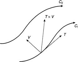
The vectors T, V, and T × V form an orthogonal frame that moves with s along C1. The derivative dV/ds is the rate of change of V along C1, and its component in the direction T × V is the scalar product (T × V) · dV/ds.
We now define the twist Tw(C2, C1) of C2 about C1 as the total change in V in the direction T × V as the curve C1 is traversed:
 (12.2)
where L is the length of C1. The factor 2π is included in order to express twist in number of turns rather than in angular change.
Note that twist is not in general an integer, and its value depends on how the curves are deformed in space, as we show later. Also, the twist of C2 about C1 is not necessarily the same as the twist of C1 about C2, although we do not show that here. Unlike the linking number, therefore, twist is not a topological invariant.
If C1 is allowed to wriggle about in space, a new quantity is introduced, called writhe, that measures how much wriggle there is. This can be done in a formal manner, as was done for link and twist. But instead it is easier to invoke a fairly deep theorem that shows how all these terms are related:
![]() (12.3)
(12.3)
The writhe of C1, Wr(C1), is defined by this relation. It can be shown to be zero for curves confined to a plane, which explains why link and twist were the same in the foregoing example.
Writhe is again dependent on how the curve is deformed and is not a topological invariant. Relation (12.3) is an intriguing mix of topological and geometrical notions that constrains how DNA can coil up.
12.3 Loopy DNA
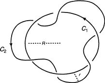
Let’s compute link, twist, and writhe in a specific case. Choose C1 to be a circle of radius R and length L = 2πR. Construct a torus (inner tube, if you wish) of radius r smaller than R having C1 as its central axis. Let C2 be a helical curve that lies on the surface of the tube so that it winds about C1 n times. Figure 12.3 illustrates the configuration of the two curves in the case of n = 3.
Assume, more generally, that C1 is a smooth closed curve lying in a plane that does not cross itself and defined, in terms of arc-length s, by the vector function x(s). Moreover, let y(s) define a helical curve C2 that wraps around C1 on a tube of radius r centered at x(s). Then
![]()
where V(s) is a unit vector, to be defined momentarily, that is directed from a point on C1 to a corresponding point on C2.
Take a cross-sectional slice of the torus by passing a plane through x(s), orthogonal to the unit tangent vector T to C1 at x(s). Choose N to be a unit normal to C1 at x(s), lying in the plane of the curve, and let B denote T × N. Then B is a unit vector orthogonal to the plane containing C1; N and B together determine the slicing plane. This follows from the well-known Frenet–Serret apparatus of space curves. If a curve C is represented parametrically by r(s), with arc-length s, then T = dr/ds is a unit tangent to the curve at all points on C defined by the parameter s. Since T · T = 1 everywhere on C, the derivative of this scalar product is zero, and so T · dT/ds = 0. The length of dT/ds is called the curvature, and therefore dT/ds = kN, where N is a unit normal to the curve (and orthogonal to T). Let B = T × N. Since T and N have unit length, so does B, from the way a cross product of two vectors is defined. To see this, if curve C lies in the x, y plane, then so does its tangent, and therefore T(s) = (x(s), y(s), 0). It follows that dT/ds = (x′(s), y′(s), 0) lies in the same plane. Since B is orthogonal to T and N, it points in the z direction with constant length of 1. That is, B = (0, 0, 1), and so dB/ds = 0 along C. Since B, T, and N are orthogonal, 0 = d(B · N)/ds = B′ · N + B · N′ = B · N′, from which it follows that N′ is orthogonal to B = N′ is also orthogonal to N, since it has constant unit length along C. Therefore, N′ is some multiple β of T. Now, 0 = d(N · T)/ds = N′ · T + N · T′ = N′ · T + k (since T′ = kN); we see from this that N′ · T = –k. Using the fact that N′ = βT, we get β = –k, and therefore N′ = –kT, as required.
Now, if C lies entirely in a plane, then T and N also lie in the same plane, from which it follows that B is a constant unit-length vector perpendicular to the plane. That is, dB/ds = 0 along C. Now show that dN/ds = –kT for planar curves.
Define the unit vector V(s) by cos(αs)N + sin(αs)B, where α = 2n/L. Then y(s) = x(s) + rV(s) is indeed a point on C2; the quantity αs measures the angle from N to y(s) (Figure 12.4). There is, therefore, a one-to-one correspondence between C1 and C2 in which a point on C1 defined by x(s) is uniquely identified with a point on C2 defined by y(s) for each value of s from 0 to L. As s moves along C1, the vector y(s) rotates about C1 and generates the helical curve C2 that lies on the tube of radius r centered at x(s).
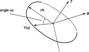
FIGURE 12.4 A plane slicing a torus whose central axis is a curve that is intersected orthogonally by the plane.
The vector B is constant along C1, and so dB/ds = 0. In fact,
![]()
However, B′ = 0 and N′ = –kT. Formula (12.4) now follows:
![]() (12.4)
(12.4)
where k is the curvature of C1, defined as the length of the vector dT/ds (incidentally, we have implicitly assumed all along that r is smaller than the radius of curvature k so that the tube does not intersect itself).
We know that B = T × N, and it is easy to check that T × B = –N. So T × V = cos(αs)B – sin(αs)N. We therefore obtain
![]()
We are now ready to compute the twist using (12.2). This gives us
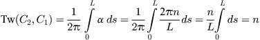
In this example, linking and twist are the same. But this is not generally the case, provided that C1 is allowed to wriggle.
Although it is possible to carry out some computations to evaluate writhe in specific cases, similar to but more demanding than the calculation already done, it is more expedient to invoke our intuition at this juncture. Consider Figure 12.5. In the first panel (panel a) the link, twist, and writhe are all evidently zero, but in panel b the twist of C2 about C1 is still zero, but the writhe of C1 is not zero, since the curve loops up and over itself out of the plane. In fact, the curves have a linking number of +1, and formula (12.3) shows that the writhe is also +1. Now deform C1 so that it doesn’t loop out of the plane by undoing the loop of the ribbon up and over itself. The linking number remains unchanged under this deformation, and we get the configuration of panel c, in which the writhe is now zero (C1 is planar) but the twist is +1. To verify the transition from b to c or back from c to b, simply take a piece of ribbon, give it a single twist, and tape the ends together. Try it!
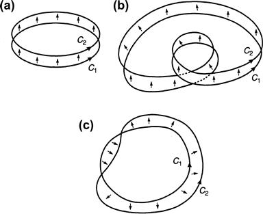
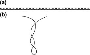
It is evident from these examples that as the curves are deformed in space, writhing and twisting are interchangeable quantities, even if the linking number remains unaltered. A more familiar example of this phenomenon is provided by grasping an ordinary string at its two ends, pulling it tight, and then twisting it. The writhing is essentially zero, but the twist is considerable and can be felt in our fingers. Now bring the hands together. The twist seems to relax palpably, but the string loops (Figure 12.6) to form what is called a superhelix. The twist has now decreased, but the writhe is substantial. The same phenomenon is observed in a coiled telephone wire (when was the last time you saw one of those?) if you stretch it out. In this case, one goes from high writhe and low twist to just the opposite.
12.4 The Gauss Linking Number
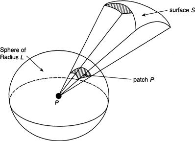
Lines emanating from a point p that intersect a segment of a smooth curve in a plane subtend an angle θ = s/R on a circle of radius R having p as its center, where s is the arc-length of the segment of the circle that is intersected by the lines (Figure 12.7). This can be extended to three dimensions to form a solid angle, in the following manner. All the lines that emanate from a point p in space and intersect a segment S of smooth surface form a cone that intersects a sphere of radius L in a patch P of area A(P) (Figure 12.7). The solid angle with vertex p subtended by S is defined to be Ω(p) = A(P)/L2.
Let r denote the position vector from p to any point of the surface S. In terms of coordinates, if p = (a, b, c), then r = (x – a, y – b, z – c), and we define γ as the scalar product r · r = (x – a)2 + (y – b)2 + (z – c)2.
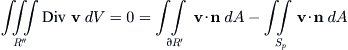
Consider the closed region R enclosed by S, P, and the surface of the cone between P and S (Figure 12.7), and let n denote the unit outward normal to R. Define a vector field v by r/γ3/2. Then the divergence theorem of vector calculus tells us that
![]()
where ∂R indicates the boundary of R consisting of the S ∪ P ∪ boundary of the cone. It is a straightforward computation to show that Div v = 0. Since n is orthogonal to r (and therefore to v) along the boundary of the cone, the double integral over this part of the boundary of R vanishes. Moreover, n is collinear to v but points in the opposite direction on P where γ = L2. It follows that
![]() (12.5)
(12.5)
The left side of this expression is simply the solid angle Ω(p), and so
![]() (12.6)
(12.6)
An immediate consequence of (12.6) is that the solid angle does not depend on the radius L of the sphere, and so we can conveniently choose the radius to be 1 from now on.
Let ∂(S) denote the bounding curve of the surface segment S, and suppose that S′ is any other smooth surface segment having the same boundary ∂(S). Call R′ the region enclosed by S ∪ S′. If p is outside R′, then the same argument that led to (12.5), using the divergence theorem, now shows that
![]() (12.7)
(12.7)
and, therefore, in view of (12.6), the solid angle depends only on the boundary of a surface and not on the surface segment itself. Moreover, because Ω(p) is the double integral of v · n over R′, and because S and S′ are arbitrarily chosen surfaces, (12.7) shows that Ω(p) = 0 for p outside any closed surface, which, in this case, is ∂R′.
On the other hand, if p is inside R′, then choose a small sphere Sp about p entirely enclosed within R′, and consider the annular region R″ lying between the outside of Sp and the boundary of R′. The previous argument now shows that
The integral of v · n on the right reduces to 1/γ ∫∫sp dA because v = r/γ3/2 = n/γ (note that v and n are collinear on Sp). But the double integral equals the area of Sp, namely, 4πγ, from which it follows that the integral of v · n over the boundary of R′ is 4π. Thus Ω(p) = 4π whenever p is inside a closed surface, which in this case is ∂R′. This fact will prove useful momentarily.
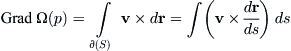
We leave it as a somewhat tedious exercise to establish, using Stokes’ Theorem, that
 (12.8)
where Grad means “gradient of,” v × dr/ds denotes the cross product of the two vectors, and the integral on the right is a line integral with respect to arc-length s over the bounding curve ∂S.
We now come to our main point: Let C1 and C2 be two smooth closed curves that link each other. We want to count the number of times they are entwined.
Suppose that C1 bounds a surface S, and let n1 be the number of times C2 pierces S in the direction shown in Figure 12.8 (for simplicity, think of C2 as lying in the x, y plane, bounding a portion of the plane, with C2 crossing this plane from z > 0 to z < 0). In the same manner, let n2 be the number of times C2 crosses from z < 0 to z > 0. The linking number Lk(C1, C2) is defined as n1 – n2.
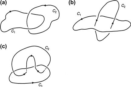
In Figure 12.8a the linking number is +1 because n1 = 1 and n2 = 0, whereas the linking number of Figure 12.8b is 0 because n1 and n2 are both 1. Finally, in Figure 12.8c, the linking number is –2 because n1 = 0 and n2 = 2. We now show how Lk(C1, C2) can be expressed as an integral.
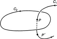
It is fairly evident that Ω(p) changes in a continuous manner as p moves along C1 and that the only source of discontinuity would occur when p penetrates S. To see what happens, attach a second surface, S′, to the same boundary C2 so that S ∪ S′ encloses a region R. Let p′ be some other point on C1 that lies on a different side of S than does p and that is outside R, whereas p lies inside (Figure 12.9). As before, n denotes the outward unit normal to the closed surface S ∪ S′.
Using the divergence theorem together with relation (12.6), it was seen earlier that Ω(p) = 4π, whereas Ω(p′) = 0 for the closed surface ∂R = S ∪ S′. The outward normal n points in the opposite direction to the normal of the surface S as defined by the orientation of its boundary C2, and therefore, as was seen earlier, Ω(p) equals both ![]() and
and ![]() , which we write as ΩS(p) and ΩS′(p), respectively. Thus, ΩS(p) – ΩS′(p) = 4π and ΩS(p′) – ΩS′(p′) = 0. Subtract the second of these identities from the first to obtain
, which we write as ΩS(p) and ΩS′(p), respectively. Thus, ΩS(p) – ΩS′(p) = 4π and ΩS(p′) – ΩS′(p′) = 0. Subtract the second of these identities from the first to obtain
![]() (12.9)
(12.9)
Observe that the solid angle can be positive or negative, depending on whether the angle between v to n is acute or obtuse. Since p and p′ lie on the same side of S′, by the way we positioned them (Figure 12.9), the last two terms in (12.9) have the same sign. Therefore they cancel in the limit as p – p′ shrinks to zero. From (12.9) it now follows that as p approaches p′, Ω(p) tends to Ω(p′) + 4π. Thus, each time C2 loops through C1 by piercing S from above, the solid angle Ω(p) jumps by 4π, and it decreases by 4π when it pierces S from below. It follows that the total change in Ω as p traverses C2 through one complete circuit is a multiple of 4π:
![]() (12.10)
(12.10)
where the integral on the right is a line integral with respect to arc length τ. The point p that traverses C2 through one cycle is parameterized by a position vector r2(τ). Points on C1, on the other hand, are parameterized by a position vector r1(s) with parameter s. Now, v = r/γ3/2, with r = r2 – r1 being a vector directed from a generic position p on C2 to some other point on C1; the length of r is γ1/2.
Using the chain rule of differentiation, dΩ/dτ = Grad Ω(p)·dr2/dτ. Employing (12.10) finally shows that
![]()
The vectors dr1/ds and dr2/dτ are tangents to C1 and C2 and can be written as T1, T2, respectively. Noting that (v × T2)·T1 = v·(T2 × T1) gives us the expression we are looking for:
![]() (12.11)
(12.11)
Expression (12.11), known as Gauss’s linking formula or, simply, as Gauss’s integral, is often written as Lk(C1, C2). It is evidently always an integer, positive or negative. Although it is fairly clear on intuitive grounds that Lk(C1, C2) = Lk(C2, C1), this also follows from (12.11), since a reversal of the roles of the two curves also reverses the sign of v, and, moreover, T2 × T1 = –T1 × T2, so that integral is unchanged.
The derivation of Gauss’s formula did not depend on how C1 and C2 are deformed in space as long as neither is allowed to intersect the other during a deformation. This means that the linking number is a topological invariant.
The Gauss linking formula will not be used explicitly in what follows because the linking number will be clear from the applications. However, its derivation is a prototype of the kind of mathematics that is needed for more profound investigations into the geometry and topology of DNA.
12.5 Concluding Thoughts
Good background reading for DNA coiling is the Scientific American article by Bauer, Crick, and White [10] and Cipra’s review in Science [34]. More technical details are provided in the article by White and Bauer [119], while a proof of relation (12.3) can be found in a paper by James White [118]. An interesting discussion of the historical origins of the linking formula and its connection to James Clerk Maxwell is contained in Epple’s note [45].
The somewhat incomplete proof of Gauss’s formula (12.11) of Section 12.4 follows the one to be found in the book on multivariate calculus by Courant and John [38].
We know that Lk(C1, C2) = Lk(C2, C1). Reversing the roles of the two curves in (12.3), we see that Tw(C1, C2) – Tw(C2, C1) = Wr(C2) – Wr(C1). In the example carried out in Section 12.3, in which C1 is a circle and C2 is a helix wound about C1, it is possible to compute the writhe of C2 using the preceding relation between twist and writhe. It can be shown (see the paper by White and Bauer [119]) that Tw(C1, C2) is approximately nL/(L2 + 4π2n2r2)1/2, or, regrouping terms, Wr(C2) is approximately n[1 – (1 + 4πnr/L)2]–1/2. This illustrates the fact that the twist of one curve about another is not necessarily the same if the two curves are interchanged.