
Nonlinear Differential Equations and Oscillations
In Section 8.3 we discussed systems of linear differential equations of the form x′ = Ax. These are written in vector notation in which A is the matrix of coefficients and the prime ′ indicates differentiation. Our interest in these equations stems from the fact that the local behavior of solutions of a nonlinear system of differential equations x′ = f(x) about some equilibrium solution is determined by the global behavior of the linearized system x′ = Ax, where A now indicates the Jacobean matrix of f.
Suppose x is an equilibrium point of x′ = f(x), with f(x) = 0. If solutions that begin nearby to x return to this point as t increases, we say that the equilibrium is an attractor or, as it is sometimes called, a sink. The next theorem is a local result, since it asserts that x is an attractor when solutions begin in some sufficiently small neighborhood of x. First, let u = x – x so that, by Taylor’s theorem, f(x) = f(x + u) = Au + g(u), where A is the Jacobean matrix of f at x and g(u) consists of higher-order terms in u that go to zero faster than u, namely, ![]() . The equations u′ = Au are called the linearized system corresponding to x′ = f(x).
. The equations u′ = Au are called the linearized system corresponding to x′ = f(x).
Note that in the case of two-dimensional systems, the condition that the eigenvalues of A have negative real parts translates into trace A < 0 and determinant A > 0.
The results just stated are given without proof since lucid arguments can be found, together with the relevant linear algebra, in the book by Hirsch, Smale, and Devaney [62], especially Chapter 8. Our goal in this appendix is to provide some details regarding the formation or existence of cyclic solutions.
Before doing so, a few preliminaries are in order. Many dynamical systems consist of three differential equations, in which the Jacobean matrix A has two complex-conjugate eigenvalues and one real eigenvalue. A starting point for the investigation of such systems is to express the linearized system x′ = Ax in a particular form to be described next.
Let the eigenvalues be α ± iβ and real λ, with corresponding eigenvectors u ± iv, w. Then A(u ± iv) = (i ± iβ)(u ± iv), so Au = αu – βv and Av = βu + αv. The real eigenvectors u, v are linearly independent. Thus, R3 is the direct sum of two subspaces of dimensions 1 and 2, spanned by w in one case and by u, v in the other, and each subspace is invariant under A.
Let T be the real matrix with columns w, u, v. Then AT = TΛ, where
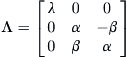
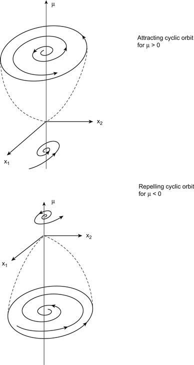
If x = Tz, then x′ = ATz and z′ = (T –1AT)z = Λz. Thus, relative to the real basis T, the linear system z′ = Λz has the form
Evidently, this linear system is asymptotically stable, provided that λ and α are both negative. Let me add, as an aside, that though the concept of a point attractor has meaning in physical systems, for biological and social aggregates the notion of a stable equilibrium is less acceptable because it is tantamount to stagnation. At best, organic entities hover about an equilibrium and, indeed, are more likely to be found in oscillatory patterns or, more generally, weaving somewhat erratically about several equilibrium states. These possibilities are discussed later.
Although we have focused on attracting equilibria, there are other kinds of attractors for nonlinear systems, as was already pointed out in Section 8.3. Of common occurrence in applications are cyclic attractors, or limit cycles, which are closed orbits on which x(t + T) = x(t) for some T > 0; T is the period of one cycle about the orbit. To say it is an attractor means that it consists of points p such that nearby solutions approach each such p through a sequence of increasing times tk, k = 1, 2, . . . .
For the sake of clarity I repeat here what was already stated in Section 8.3 regarding the conditions that ensure that an attracting cycle ensues from a repelling equilibrium. Consider, then, a dynamical system x′ = f(x, μ), in which f depends smoothly on x and a parameter μ. Let x(μ) be an equilibrium point. The Jacobean and its eigenvalues also depend smoothly on μ. Suppose that in some neighborhood of some μo the eigenvalues are complex, for n = 2, or consist of a complex pair and one real eigenvalue for n = 3. Denote the complex eigenvalues by α(μ) ± iβ(μ) and the real value by λ. Suppose that the following conditions hold at x(μo):
![]()
Then there is a cyclic orbit about x(μ) for all μ in some neighborhood of μo, whose amplitude increases with the magnitude of μ. This is called a Hopf bifurcation, and μo is a bifurcation point. Note that the second of these conditions guarantees that the real part of the complex eigenvalues actually crosses the imaginary axis as μ passes its critical value.
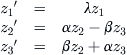
Generally, the loss of stability at μo is such that α(μ) < 0 for μ < μo (with λ3 < 0 for n = 3) and α(μ) > 0 for μ > μo. In this case the equilibrium is an attractor for μ < μo and a repeller for μ > μo. However, whether the cyclic orbit itself is attracting or not depends on the higher-order terms in f(x, μ) and is more difficult to determine. In fact, the cycle can be attracting for μ > μo and repelling for μ < μo, or vice versa, as illustrated in Figure C.1.
In most settings the loss of stability and the onset of stable fluctuations can be observed directly. It suffices to verify these conditions, since these lend plausibility to the model as a characterization of the underlying phenomenon, and it assists in computing the bifurcation value. The main purpose of the analysis is to verify that conditions for the onset of oscillations are present, which makes the model a credible metaphor for what is actually observed to take place.
A sketch of the essential steps of a proof of the bifurcation theorem, following Loud [75], will be given shortly. It applies to planar systems. But if the single real eigenvalue remains negative even when μ exceeds the critical threshold in the three-dimensional system, then the resultant instability is now effectively due to the two-dimensional system’s having complex conjugate eigenvalues, as I sketch shortly, and so the proof I give in this appendix remains valid for three-dimensional models. The proof is somewhat lengthy, but I include it here because it is rarely found in an introductory course on nonlinear differential equations.
First, however, let’s give a simple example of a Hopf bifurcation in terms of the Van der Pol equation, which arose in a study of vacuum tube oscillators in 1927:
![]()
Letting x1 = y and x2 = y′ we obtain a first-order nonlinear system of equations:
![]()
There is an equilibrium at x = 0, and the Jacobean at this point is
![]()
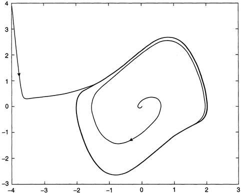
The determinant of A is positive, and the trace is μ; therefore the origin in the plane is an attractor for μ < 0. Let’s consider what happens when μ > 0. The roots of Det (A – λI ) = 0 satisfy the quadratic polynomial λ2 – μλ + 1 = 0, and it is easy to check that they are complex conjugate for μ small enough. The real parts are zero at μ = 0, but the imaginary part is nonzero there. Moreover, the derivative with respect to μ is nonzero at μ = 0, so the conditions for a Hopf bifurcation are met. Oscillations are actually encountered when the equations are integrated numerically, and so we surmise that there is a stable limit cycle that attracts all orbits in the vicinity of the origin when μ is small and positive (Figure C.2).
Now we are ready to sketch the proof of the bifurcation theorem. The eigenvalues of the linearized system are taken to be complex conjugate a ± ib, and we put the linear part of the equations into form
![]() (C.1)
(C.1)
with x = y = 0 being an equilibrium solution. We also assume that
![]()
Let x(t, s, z) and y(t, s, z) indicate solutions of (C.2) for which x = s and y = 0 at time z = 0. We then look for solutions that begin at s and return later to the x-axis at a time z + 2π. Define functions
![]() (C.2)
(C.2)
The solution beginning on the real axis at x = s will be periodic with period z + 2π if and only if F = G = 0. Since x(t, 0, μ) = y(t, 0, μ) = 0 for all μ, then F(z, 0, μ) = G(z, 0, μ) = 0. Now write F and G as F(z, s, μ) = sF1(z, s, μ) and G(z, s, μ) = sG1(z, s, μ).
I show later that G1s(0, 0, 0) = 1, and so we can solve locally for z as a function of s and μ:
![]() (C.3)
(C.3)
Therefore, the time of return of the orbit to the x-axis, when it begins at x = s and y = 0, is H(s, μ) + 2π, and the displacement of the orbit from the starting point s on the x-axis is
![]() (C.4)
(C.4)
If (C.4) is positive, the solution returns to a point to the right of s on the x-axis; otherwise, for a negative (C.4), it returns to the left of s, as shown in Figure C.3.
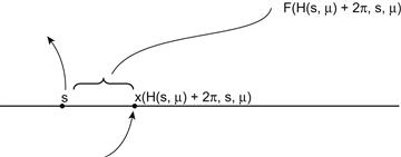
FIGURE C.3 First return of the orbit (C.5).
We now express F(H(s, μ), s, μ) as sF1(H(s, μ, s, μ)) = sJ(s, μ). Then the condition for a closed periodic orbit becomes J(s, μ) = 0. To move forward we need to develop an explicit expression for J.
The partial derivatives of F1 and G1 at (0, 0, 0) are found by computing the derivatives of x and y at s = μ = 0. To begin this process, observe that when t = z + 2π, one obtains, from (C.2), that
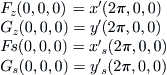 (C.5)
(C.5)
To evaluate the last two relations in (C.5), note that
![]() (C.6)
(C.6)
At t = 0 one has x = s and y = 0, and so xs = 1 and ys = 0 are the initial conditions for Equations (C.6).
When s = μ = 0 in (C.6), the equations reduce, using (C.1), to
![]()
whose solution is xs(t, 0, 0) = cos t and ys(t, 0, 0) = sin t. At t = 2π we see that xs = 1 and ys = 0. Therefore, the last two relations of (C.5) become
![]()
Moreover, since F = sF1, then Fs = sF1s + F1, with a similar expression for Gs. It follows that
![]()
Continuing in this fashion, one gets, further,
![]()
and especially, after some tedious computations,
![]() (C.9)
(C.9)
It follows that G1(z, s, μ) = G1(0, 0, 0) +G1z(0, 0, 0)z + G1s(0, 0, 0)s + G1μ(0, 0, 0) + higher-order terms in s and μ. Thus, G1(z, s, μ) = z + 2πb′(0)μ + ![]() and, therefore, z = H(s, μ) = –2πb′(0)μ for s, μ small enough.
and, therefore, z = H(s, μ) = –2πb′(0)μ for s, μ small enough.
We now approach the endgame in our proof, since it easily follows from the foregoing expression that H(0, 0) = 0, Hs(0, 0) = 0, and Hμ(0, 0) = –2πb′(0) and, from this, J(s, μ) = J(0, 0) + Js(0, 0)s + Jμ(0, 0)μ + Jss(0, 0)s2/2 + higher-order terms in s and μ. Let’s assume the generic case in which Jss(0, 0) is nonzero. Then, to evaluate the terms in the expansion of J, recall that J(s, μ) = F1(H(s, μ), s, μ). From this it is easily established, using the previously computed derivatives of F1, that
![]()
We know from (C.1) that a′(0) > 0, and so, provided that s, μ are small enough and that Jss(0, 0) < 0, J(s, μ) has two solutions for μ > 0:
![]()
for some scalar c, with s– < 0 < s+
These s values represent the intersection of the closed orbit with the x-axis as it crosses at two points, once upward and once downward, with the first being the starting point. If 0 < s < s+, then
![]()
whereas [assuming, again, that Jss(0, 0) < 0] if s > s+, then J(s, μ) < 0. This means that the displacement sJ(s, μ) is positive (negative) for s < s+ (s > s+), which tells us that an orbit starting at s on the x-axis will cross the axis again at a location closer to s+. Consequently, the closed orbit is a stable cycle.
When μ = 0 and Jss(0, 0) < 0, the same reasoning establishes that the origin is a local attractor that becomes repelling for μ > 0, with solutions tending to the limit cycle. Note that the radius of the cycle increases as √μ. There are similar, but less interesting, consequences for the case Jss(0,0) > 0 in terms of cycles for μ < 0. These results, we repeat, are valid only for s and μ sufficiently small.
When a system loses stability as the bifurcation parameter exceeds a threshold in a three- or higher-dimensional system, there are typically only two complex eigenvalues associated with this change. The central idea of bifurcation theory is that the dynamics of the system near the onset of instability is governed by the evolution of the two equations associated with these complex eigenvalues, while the remaining equations follow in a passive fashion; that is, they are “enslaved.” The center manifold theorem is the rigorous formulation of this idea; it allows us to reduce a large problem to a small and manageable one (see the first two chapters of Carr’s book Applications of Centre Manifold Theory, Springer-Verlag, 1981).
To be more specific, consider the system of three equations whose linear parts can be written in the form (C.1) in which the coefficients a, b are the real and imaginary parts of a complex eigenvalue and λ is real. These coefficients depend on a parameter μ, and the usual Hopf conditions apply at the origin, where a bifurcation takes place at μ = 0:
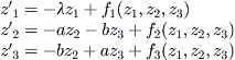
Depending on certain smoothness assumptions, there exists, in some sufficiently small neighborhood of the origin, a smooth surface z1 = h(z2, z3) called the center manifold such that every solution that begins on this surface remains on it. The system of equations is now reduced to
![]()
The variable z1 has effectively been entrained by the behavior of z2 and z3 near the equilibrium point.