
Crabs and Criminals
1.1 Background
A hand reaches into the still waters of the shallow lagoon and gently places a shell on the sandy bottom. We watch. A little later a tiny hermit crab scurries out of a nearby shell and takes possession of the larger one just put in. This sets off a chain reaction in which another crab moves out of its old quarters and scuttles over to the now-empty shell of the previous owner. Other crabs do the same, until at last some barely habitable shell is abandoned by its occupant for a better shelter, and it remains unused.
One day the president of a corporation decides to retire. After much fanfare and maneuvering within the firm, one of the vice presidents is promoted to the top job. This leaves a vacancy, which, after a lapse of a few weeks, is filled by another executive, whose position is now occupied by someone else in the corporate hierarchy. Some months pass, and the title of the last position to be vacated is merged with some currently held job title and the chain terminates.
A lovely country home is offered by a real estate agency when the owner dies and his widow decides to move into an apartment. An upwardly mobile young professional buys it and moves his family out of the split-level they currently own after selling it to another couple of moderate income. That couple sold their modest house in a less-than-desirable neighborhood to an entrepreneurial fellow who decides to make some needed repairs and rent it.
What do these examples have in common? In each case a single vacancy leaves in its wake a chain of opportunities that affect several individuals. One vacancy begets another as individuals move up the social ladder. Implicit here is the assumption that individuals want or need a resource unit (shells, houses, or jobs) that is somehow better (newer, bigger, more status) or, at least, no worse than the one they already possess. There are a limited number of such resources and many applicants. As units trickle down from prestigious to commonplace, individuals move in the opposite direction to fill the opening created in the social hierarchy.
A chain begins when an individual dies or retires or when a housing unit is newly built or a job created. The assumption is that each resource unit is reusable when it becomes available and that the trail of vacancies comes to an end when a unit is merged, destroyed, or abandoned, or because some new individual enters the system from the outside. For example, a rickety shell is abandoned by its last resident, and no other crab in the lagoon claims it, or else a less fortunate hermit crab, one who does not currently have a shell to protect its fragile body, eagerly snatches the last shell.
A mathematical model of movement in a vacancy chain is formulated in the next section and is based on two notions common to all the examples given. The first notion is that the resource units belong to a finite number, usually small, of categories that we refer to as states; the second notion is that transitions take place among states whenever a vacancy is created. The crabs acquire protective shells formerly occupied by snails that have died, and these snail shells come in various size categories. These are the states. Similarly, houses belong to varying price/prestige categories, while jobs in a corporate structure can be labeled by different salary/prestige classes.
Let’s now consider an apparently different situation. A crime is committed, and, in police jargon, the perpetrator is apprehended and brought to justice and sentenced to “serve time” in jail. Some crimes go unsolved, however, and of the criminals that get arrested only a few go to prison; most go free on probation or because charges are dropped. Moreover, even if a felon is incarcerated or is released after arrest or even if he was never caught to begin with, it is quite possible that the same person will become a recidivist, that is, a repeat offender. What this has in common with the mobility examples given earlier is that here, too, there are transitions between states, where in this case “state” means the status of an offender as someone who has just committed a crime, has just been arrested, has just been jailed, or, finally, has “gone straight,” never to repeat a crime again. This, too, is a kind of social mobility, and we will see that it fits the same mathematical framework that applies to the other examples.
One of the problems associated with models of social mobility is the difficult chore of obtaining data regarding the frequency of moves between states. If price, for example, measures the state of housing, then what dollar bracket constitutes a single state? Obviously the narrower we make a price category, the more homogeneous is the housing stock that lies within a given grouping. On the other hand, this homogeneity requires a large number of states, which exacerbates the data-gathering effort necessary to estimate the statistics of moves between states.
We chose to tell the crab story because it is a recent and well-documented study that serves as a parable for larger-scale problems in sociology connected with housing and labor. It is not beset by some of the technical issues that crop up in these other areas, such as questions of race that complicate moves within the housing and labor markets. By drastically simplifying the criminal justice system, we are also able to address some significant questions about the chain of moves of career criminals that curiously parallel those of crabs on the sandy sea bottom. These examples are discussed in Sections 1.3 through 1.5.
More recent work on crab mobility shows that, in contrast to the solitary crab behavior discussed earlier in which a single individual searches for a larger shell before vacating its existing home, the terrestrial hermit crab Coenobita clypeatus engages in a more aggregate behavior, in which a cluster of crabs piggyback each other in order to move together as a group. The crabs grasp the shell of another denizen from behind, with the leader dragging itself along trailed by a queue of expectant crabs. Because they move as a group, then at the moment the largest of them finds a shell, the others have immediate access to the collection of discarded shells all in proximity to one another, as the crabs quickly discard and acquire new homes. This is reminiscent of the rental market for student apartments in the first few days of the beginning of the fall semester in a college town as some students move out and others frantically move in.
This queuing behavior of the crabs has several features in common with queues in general, such as the formation of multiple waiting lines of clinging crabs that jockey for position between clusters. The advantage of this social activity is that it increases the likelihood of finding an appropriate shell, since many become available in short order, but this is offset by the risk that these aggregates are now more vulnerable to predation.
1.2 Transitions Between States
We began this chapter with examples of states that describe distinct categories, such as the status of a felon in the criminal justice system or the sizes of snail shells in a lagoon. Our task now is to formalize this idea mathematically.
The behavior of individual crabs or criminals is largely unpredictable, and so we consider their aggregate behavior by observing many incidents of shell swapping or by examining many crime files in public archives.
Suppose there are N states and that pi,j denotes the observed fraction of all moves from a given state i to all other states j. If a large number of separate moves are followed, the fraction pi,j represents the probability of a transition from i to j. In fact this is nothing more than the usual empirical definition of probability as a frequency of occurrence of some event. The N-by-N array P with elements pi,j is called a transition matrix.
To give an example, suppose that a particle can move among the integers 1, 2, . . . , N by bouncing one step at a time either right or left. If the particle is at integer i, and it goes to i + 1 with probability p and to i – 1 with probability q, then p + q = 1, except when i is either 1 or N. At these boundary points the particle stays put. It follows that the transition probabilities are given by
![]()
The set of transitions from states i to states j, called a random walk with absorbing barriers, is illustrated schematically in Figure 1.1 for the case N = 5.
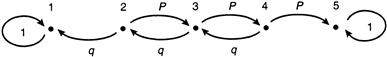
A Markov chain (after the Russian mathematician A. Markov) is defined to be a random process in which there is a sequence of moves between N states such that the probability of going to state j in the next step depends only on the current state i and not on the previous history of the process. Moreover, this probability does not depend on when the process is observed. The random-walk example is a Markov chain, since the decision to go either right or left from state i is independent of how the particle got to i in the first place, and the probabilities p and q remain the same regardless of when a move takes place.
To put this in more mathematical terms, if Xn is a random variable that describes the state of the system at the nth step, then prob(Xn+1 = j | Xn = i), which means “the conditional probability that Xn+1 = j given that Xn = i” is uniquely given by pi,j. In effect, a move from i to j is statistically independent of all the moves that led to i and is also independent of the step we happen to stumble on in our observations. Clearly pi,j ≥ 0 and, since a move from state i to some other state always takes place (if one includes the possibility of remaining in i), then the sum of the elements in the ith row of the matrix P add to 1:
![]()
The extent to which these conditions for a Markov chain are actually met by crabs or criminals is discussed later. Our task now is to present the mathematics necessary to enable us to handle models of social mobility. A state i is called absorbing if it is impossible to leave it. This means that pi,i = 1. In the random-walk example, for instance, the states 1 and N are absorbing.
Two nonabsorbing states are said to communicate if the probability of reaching one from the other in a finite number of steps is positive. Finally, an absorbing Markov chain is one in which the first s states are absorbing, the remaining N – s nonabsorbing states all communicate, and the probability of reaching every state i ≤ s in a finite number of steps from each i′ > s is positive.
It is convenient to write the transition matrix of an absorbing chain in the following block form:
![]() (1.1)
(1.1)
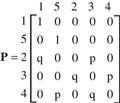
where I is an s-by-s identity matrix corresponding to fixed positions of the s absorbing states, Q is an (N – s)-by-(N – s) matrix that corresponds to moves between the nonabsorbing states, and R consists of transitions from transient to absorbing states. In the random walk with absorbing barriers with N = 5 states (Figure 1.1), for example, the transition matrix may be written as
Let P(n) be the matrix of probabilities ![]() of going from state i to state j in exactly n steps. This is conceptually different from the n-fold matrix product Pn = PP . . . P. Nevertheless they are equal:
of going from state i to state j in exactly n steps. This is conceptually different from the n-fold matrix product Pn = PP . . . P. Nevertheless they are equal:
Proof
Let n = 2. A move from i to j in exactly two steps must pass through some intermediate state k. Because the passages from i to k and then from k to j are independent events (from the way a Markov chain was defined), the probability of going from i to j through k is the product pi,k pk,j (Figure 1.2). There are N disjoint events, one for each intermediate state k, and so
![]()
which we recognize as the i,jth element of the matrix product P2.

We now proceed to the general case by induction. Assume the lemma is true for n – 1. Then an identical argument shows that
![]()
which is the i, jth element of Pn.
1.3 Social Mobility
The tiny hermit crab, Pagurus longicarpus, does not possess a hard protective mantle to cover its body, and so it is obliged to find an empty snail shell to carry around as a portable shelter. These empty refuges are scarce and only become available when their occupant dies.
In a recent study of hermit crab movements in a tidal pool off Long Island Sound (see the references to Chase and others in Section 1.6), an empty shell was dropped into the water in order to initiate a chain of vacancies. This experiment was repeated many times to obtain a sample of over 500 moves as vacancies flowed from larger to generally smaller shells. A Markov chain model was then constructed using about half this data to estimate the frequency of transitions between states, with the other half deployed to form empirical estimates of certain quantities, such as average chain length, that could be compared with the theoretical results obtained from the model itself. The complete set of experiments took place over a single season during which the conditions in the lagoon did not alter significantly. Moreover each vacancy move appeared to occur in a way that disregarded the history of previous moves. This leads us to believe that a Markov chain model is probably justifiable, a belief that is vindicated somewhat by the comparisons between theory and experiment to be given later.
There are seven states in the model. When a crab that is presently without a shelter occupies an empty shell, a vacancy chain terminates, and we label the first state to be a vacancy that is taken by a naked crab. This state is absorbing. If an empty shell is abandoned, in the sense that no crab occupies it during the 45 minutes of observation time, this also corresponds to an absorbing state, which we label as state 2. The remaining five states represent empty shells in different size categories, with state 3 the largest and state 7 the smallest. The largest category consists of shells weighing over 2 g, the next size class is between 1.2 and 2 g, and so on, until we reach the smallest group of shells, which weigh between 0.3 and 0.7 g. Table 1.1 gives the results of 284 moves, showing how a vacancy migrated from shells of size category i (namely, states i > 2) to shells of size j (states j > 2) or to an absorbing state j = 1 or 2. Thus, for example, a vacancy moved nine times from a shell of the largest size (state 3) to a medium-size shell in state 5, while only one of the largest shells was abandoned (absorbing state 2).
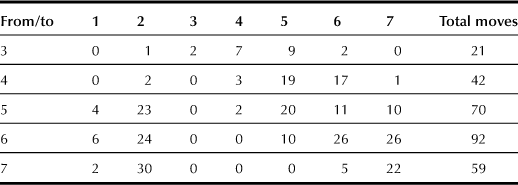
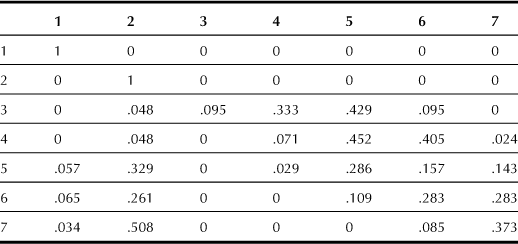
Dividing each entry in Table 1.1 by the respective row total gives an estimate for the probability of a one-step transition from state i to state j. This is displayed in Table 1.2 as a matrix in the canonical form of an absorbing Markov chain (relation 1.1).
To make further progress with this model we need to develop the theory of absorbing chains a bit more, which is done in the next section.
1.4 Absorbing Chains
Let fi be the probability of returning to state i in a finite number of moves given that the process begins there. This is sometimes called the first return probability. We say that state i is recurrent or transient if fi = 1 or fi < 1, respectively. The absorbing states in an absorbing chain are clearly recurrent and all others are transient.
The number of returns to state i, including the initial sojourn in i, is denoted by Ni. This is a random variable taking on values 1, 2, . . . . The defining properties of a Markov chain ensure that each return visit to state i is independent of previous visits, and so the probability of exactly m returns is
![]() (1.2)
(1.2)
The right side of (1.2), known as a geometric distribution, describes the probability that a first success occurs at the mth trial of a sequence of independent Bernoulli trials. In our case “success” means not returning to state i in a finite number of steps. The expected value of Ni is 1/(1 – fi), as discussed in most introductory probability texts.
The probability of only a finite number of returns to state i is obtained by summing over the disjoint events Ni = m:
![]()
With probability 1, therefore, there is only a finite number of returns to a transient state.
In the study of Markov chains, the leading question is what happens in the long run as the number of transitions increases. The next result answers this for an absorbing chain.
The submatrix Q in (1.1) is destined to play an important role in what follows. We begin by recording an important property of Q, whose proof can be found in the book by Kemeny and Snell [71]:
We turn next to a study of the matrix (I – Q)–1. Our arguments may seem to be a bit abstract, but actually they are only an application of the ideas of conditional probability and conditional expectation.
Let ti,j be the average number of times that the process finds itself in a transient state j given that it began in some transient state i. If j is different from i, then ti,j is found by computing a conditional mean, reasoning much as in Lemma 1.1. In fact, the passage from i to j is through some intermediate state k. Given that the process moves to k in the first step (with probability pi,k), the mean number of times that j is visited beginning in state k is now tk,j. The unconditional mean is therefore pi,ktk,j, and we need to sum these terms over all transient states since these correspond to disjoint events (see Figure 1.2):
![]()
In the event that i = j, the value of ti,i is increased by 1 since the process resides in state i to begin with. Therefore, for all states i and j for which s < i, j ≤ N,
![]() (1.3)
(1.3)
where δi,j equals 1 if i = j and is zero otherwise. In matrix terms, (1.3) can be written as T = I + QT, where T is the (N – s)-by-(N – s) matrix with entries ti,j. It follows that T = (I – Q)–1.
Let ti be a random variable that gives the number of steps prior to absorption, starting in state i. The expected value of ti is
![]() (1.4)
(1.4)
which is the ith component of the vector Tc, where

and T = (I – Q)–1. Vector Tc has (N – s) components, and the ith one can therefore be interpreted as the average number of steps before absorption when a chain begins in transient state i.
The probability bi,j that absorption occurs in state j ≤ s, given that it began in some transient state i, can now be computed. Either state j is reached in a single step from i (with probability pi,j) or there is first a transition into another transient state k, and from there the process is eventually absorbed in j (with probability bk,j). The reasoning is similar to that employed earlier. That is, since the moves from i to k and then from k to j are independent by our Markov chain assumptions, we sum over (N – s) disjoint events corresponding to different intermediate states k:
![]() (1.5)
(1.5)
In matrix terms, (1.5) becomes B = R + QB, where R and Q are defined in (1.1).
Now let hi,j be the probability that a transient state j is ever reached from another transient state i in a finite number of moves. If j differs from i, then evidently
![]()
and, because we must add 1 to the count of ti,j when i = j, in all cases we obtain
![]() (1.6)
(1.6)
In matrix terms this is expressed as T = I + HTdiag, where Tdiag is the matrix whose only nonzero elements are the diagonal entries of T = (I – Q)–1 and H is the matrix with entries hi,j. Therefore
![]()
Note, for later use, that hi,i = fi.
After this lengthy excursion through some unavoidable technicalities, let’s return to the social mobility model.
The five-by-five submatrix in the lower right of Table 1.2 is Q, and (1 – Q)–1 is easily computed using any of the matrix software packages currently available, or it can be done more painfully by hand. In either case the result is
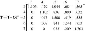
where the entries denote the average number of times ti, j that the process is in transient state j given that it began in transient i. Of interest to us are the components of the vector Tc, where c is the vector defined previously as having all entries equal to 1. These numbers give the average number of steps required for a vacancy chain to terminate, given that it starts with an empty shell of size i. For example, an average of 3.817 moves take place before absorption whenever an empty shell of the largest size category begins a chain.
Table 1.3 compares averages computed from the model with those obtained empirically through observations, and we see that there is reasonable agreement. Because no shells of size 7 were put into the water, the last entry in the first column is missing.
TABLE 1.3
Observed and Predicted Lengths of Crab Vacancy Chains
| Origin state | Observed length | Model computed length |
| 3 | 3.556 | 3.817 |
| 4 | 3.323 | 3.443 |
| 5 | 2.667 | 2.487 |
| 6 | 2.567 | 2.538 |
| 7 | 1.939 |
Finally we compute the probability that a vacancy chain terminates in state 1 or 2, given that it begins with a shell of size i. Using relation (1.5), this gives us Table 1.4.
TABLE 1.4
Probability That a Crab Vacancy Chain Ends in a Particular Absorbing State
| Origin state | Absorption state 1 | Absorption state 2 |
| 3 | .123 | .877 |
| 4 | .126 | .874 |
| 5 | .130 | .870 |
| 6 | .139 | .861 |
| 7 | .073 | .927 |
For example, if we start with a fairly small shell of size 6, the probability that the last shell in a chain remains unoccupied (abandoned) is .861. This high probability reflects the fact that shells that remain at the bottom of the chain are generally cramped and in poor condition, unattractive shelters for all but the most destitute crabs.
Each vacancy is mirrored by a crab moving to a new home, except when the last shell is abandoned (absorption in state 2). In this case, the average number of crabs moving to new quarters when a vacancy chain begins in state i is 1 less than the average vacancy chain length. When a “naked” crab takes the last shell, on the other hand, the average number of crab moves is the same as the average chain length. Conditioning on these two events, we compute the average crab mobility Mi in a chain that begins in state i. Simple considerations show that
![]() (1.7)
(1.7)
Quantity (1.7) is of interest because it provides a measure of the accumulated benefit to all crabs in a lagoon resulting from a single commodity’s becoming available. Because crab size is closely correlated to shell size, those crabs that are able to obtain less cramped shelters tend to grow larger and produce more offspring. The impact of a single vacancy has a multiplier effect because the benefits trickle down to the community of crabs. A similar conclusion would apply in chains initiated by the opening of a new job in some organization or by the sale of a home. For example, all real estate agents benefit from the sale of a single house because this triggers a bunch of other sales, and the government also benefits by being able to collect multiple sales tax payments.
The averages ti,j give an estimate of the impact that the introduction of a shell of some given size will have on the mobility of crabs and therefore on their growth and reproductive capabilities. From Table 1.3 we see that placing a large shell of type 3 into the pool benefits crabs in the intermediate state 5 more than those in state 4. Evidently the smaller crabs show a preference for a larger-than-necessary shelter and may delay their reproductive activities until such a unit becomes available. The same conclusion could apply to shrimp, octopi, and lobsters that take shelter in rock crevices and coral reef openings. Therefore, if the goal is to improve the fitness of these animals, either as a disinterested act of conservation or as a less benign attempt to provide better fishing harvests, then a useful strategy would be to place artificial shelters such as cinder blocks in an appropriate location. The problem is to estimate the benefit that certain creatures would reap from resource units of a certain size. In the case of hermit crabs, at least, the model here suggests an answer.
1.5 Recidivism
A felon who commits another crime is said to recidivate. Because a criminal is unlikely to confess to a crime unless caught, the true probability of recidivism is unknown. To the police a recidivist is someone who is rearrested, whereas the correctional system regards a recidivist as someone who returns to jail. There is a need, therefore, to clarify the meaning of these crime statistics, especially because they are often reported in the press and quoted in official reports.
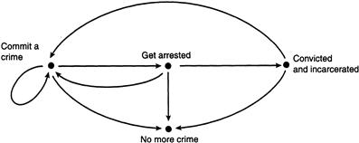
To gain some insight into this problem, a simple Markov chain model is formulated that consists of four states describing the status of an offender as seen by the criminal justice system. The first state corresponds to a former criminal who dies or decides to “go straight” and therefore, one way or the other, does not rejoin the criminal fraternity. This state is absorbing. The remaining states correspond to an individual who has, respectively, just committed a crime, just been arrested, just been incarcerated (Figure 1.3).
Let p be the true, but unknown, probability of recidivism (a criminal, not caught, commits another crime). We assume that someone who has been arrested and then released has the same propensity p to recidivate as does someone just released from jail. This means, in effect, that the future behavior of a criminal is independent of when he or she returns to society.
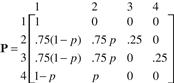
From a published paper on the subject (see the references in Section 1.6), the probability pA of being arrested, given that a crime has just been committed, is estimated to be .25, and therefore the unconditional probability of crime repetition is, in this case, p(1 – pA) = .75p. Similarly, the probability pI of being convicted, sentenced, and institutionalized, given that an arrest just took place, is also estimated to be .25. Hence the unconditional probability of crime repetition, given that an arrest took place, is p(1 – pI) = .75p. From all transient states i = 2, 3, 4 there is also a one-step absorption probability corresponding to someone returning to society as a law-abiding citizen or becoming deceased. Thus, for example, from state 2 just after a crime has been committed, the probability of no recidivism is simply (1 – p)(1 – PA). This expresses the fact that absorption into state 1 requires two independent events to hold; namely, no arrest took place after the crime was carried out and the offender’s criminal career comes to a halt.
Criminal records are prone to errors and are inherently incomplete because they do not include some arrests that may take place outside a local jurisdiction or because a central court file may fail to include arrests for minor offenses. Moreover, some individuals are falsely arrested and convicted, whereas others are dismissed from prosecution, even if arrested, because the charges are dropped due to insufficient evidence. Nevertheless, we will assume that these blemishes in the data can be disregarded and that the estimated probabilities are essentially correct. Having said this, we can write down the one-step transition matrix as
The necessary conditions for a Markov chain model are assumed to hold. This means that a move from any state is unaffected by the past criminal history of an individual and that the transition probabilities do not change over time (which is roughly true when these numbers are estimated from data sets spanning a limited number of years).
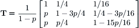
The matrix P is in the canonical form (1.1) of an absorbing chain in which the block on the lower right is Q. We can compute the 3-by-3 matrix T = (I – Q)–1 either by hand (simple enough) or by an appropriate computer code to obtain
The question of immediate interest to us is the probability of recidivism, given that an individual is in any of the transient states i = 2, 3, 4 or, to put it in other terms, the probability of ever returning to transient state i given that it begins there. Because fi = hi,i, we see from relation (1.6) that
![]()
where fi is the probability of ever returning to state i in a finite number of steps.
Therefore
![]() (1.8)
(1.8)
The i,jth component of T is ti,j, and so one need only look at the diagonal components of T to compute (1.8). The result is
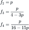
That f2 should equal p is not unexpected, because we assumed this to be true initially. Now, if p = .9, meaning there is a high likelihood of crime repetition, then the probability f3 of rearrest is .69, whereas the probability of reincarceration f4 is only .36. The different estimates of recidivism are therefore consistent with each other and simply reflect the fact that separate elements of the criminal justice system (the criminal, the police, or the corrections officer) see crime repetition from different points of view.
From T we also see that the average number of career crimes t2,2 is 1/(1 – p). When p = .9, the offender commits an average of 10 crimes during his lifetime, whereas with p = .8, there are only 5 career crimes. Thus an 11% decrease in the propensity to commit another crime can reduce the number of crimes actually carried out by 50%. This suggests that if increased vigilance on the part of the police has even a small effect in deterring a criminal, this can have a substantial impact on reducing the number of crimes actually committed.
1.6 Concluding Thoughts
A comprehensive treatment of vacancy chains in sociology can be found in the book by White [117], whereas the specific model of crab mobility discussed in Section 1.3 is taken from the papers by Chase [32] and by Weissburg and others [115]. The recent paper on the hermit crab Coenobita clypeatus that was mentioned earlier is by Rotjan et al. [101]. See, in addition, the excellent nontechnical review by Chase in Scientific American [33].
The model of Section 1.4 comes from the paper by Blumstein and Larson [22].
An excellent text on Markov chains, including absorbing chains, with many applications and proofs of all the results in this chapter is Kemeny and Snell’s book [71].
I cannot resist quoting a few lines from Dr. Seuss’s book On Beyond Zebra! (Geisel, 1955), in which he talks about creatures called Nutches who are in competition with each other. The quote is especially apt in view of how hermit crabs behave:
These Nutches have troubles, the biggest of which is
The fact there are many more Nutches than Nitches.
Each Nutch in a Nitch knows that some other Nutch
Would like to move into his Nitch very much.
So each Nutch in a Nitch has to watch that small Nitch
Or Nutches who haven’t got Nitches will snitch.
(From On Beyond Zebra! by Dr. Seuss, ™ & © by Dr. Seuss Enterprises, L.P. 1955, renewed 1983. Used by permission of Random House Children’s Books, a division of Random House, Inc.)