
Spatial Patterns
The Cat’s Tail and Spreading Slime
11.1 Background
In the previous chapter we encountered a class of models in which two separate dynamics are at work. A reaction term designates the positive growth rate of some organism or chemical within a region. The diffusion term is the rate at which this stuff is dispersed. In the specific example we considered, the algal cells are scattered to outside the region, where no growth can take place, and so reaction and diffusion oppose each other. In the present chapter these terms interact synergistically, and diffusion is the source of pattern formation and not an inhibitor.
Near the end of his life, after having completed his formidable work on computability and, later, the breaking of the enigma code, Alan Turing began a study of pattern formation in biology and wrote a seminal paper on the subject [112]. He envisaged two interacting chemicals A and B, called morphogens, of which A autocatalyzes its own production and activates the formation of B, which, in turn, acts to inhibit A. This is reminiscent of the Michaelis–Menten dynamics of blood clotting, except the reaction terms here are somewhat different. Both chemicals diffuse, but at different rates, allowing for short-range activation and long-range inhibition. How this can create a spatial pattern is indicated in Figure 11.1, in which a small perturbation of a uniformly stable spatiotemporal equilibrium density ρ gives rise to a nonuniform spatial configuration as a result of a loss of stability of the uniform state due to diffusion once certain threshold conditions are reached. This is reminiscent of a cyclic orbit generated as a Hopf bifurcation from a stable equilibrium when some parameter achieves a critical level. A remarkable feature of Turing’s model is that, though diffusion is usually a stabilizing motion, returning a system to a uniform equilibrium state and in spite of the ultimately stable reaction terms due to inhibition (much as in the blood-clotting reactions), the combination of these two separate leveling actions allow a nonuniform configuration to emerge.
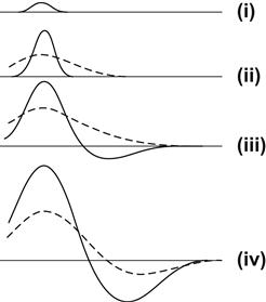
FIGURE 11.1 An intuitive demonstration of pattern formation.
In (i), a uniform distribution, the straight line is disturbed and there is a small increase in ρ. Because of autocatalysis, ρ rises further in (ii). This is accompanied by an increase in the density h of the other morphogen (dotted line). However, h spreads out faster, since its diffusion rate ν is greater than the diffusion rate of ρ. Then, in (iii), we see that wherever h is more abundant than ρ, this forces ρ to decrease even further. A decrease in ρ eventually decreases h, as shown in (iv), and so ρ can begin to rise again. In this manner, peaks and troughs eventually emerge.
Although Turing’s work remained somewhat speculative for a number of years, mainly because his use of morphogens could not be verified directly, his basic concept of diffusion-driven instability has received ample experimental verification, and now, quite recently, his work has begun to be validated in specific biological systems. The most recent example, involving the ridge pattern on the roof of the mouth of mice, clearly involves two morphogens in the manner described by Turing, as reported by Economu et al. [41]. Thus, this work on pattern formation has entered the mainstream of embryology.
I want to illustrate the essential idea of Turing’s model in the context of animal coat markings, motivated by the striped pattern on the tail of my long-deceased cat. In the next section I follow Murray’s treatment [88].
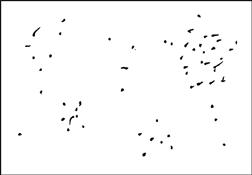
In a similar spirit to Turing’s reaction–diffusion model is a pair of equations that describe the destabilization of a uniform state of the slime mold amoeba Dictyostelium discoideum. These amoebae spread out uniformly whenever there is a plentiful supply of bacteria to feed on, usually in soil. As the food supply begins to be depleted, the amoebae start to secrete an attractant, cAMP, which tends to move the organisms toward increasing concentrations of this stimulant; as a result, pockets of slime-mold aggregates start to form, as in Figure 11.2. Startling patterns can in fact emerge consisting of colonies of amoebae that move together as a unit. Thereafter, the colonies form a slug that ultimately forms new spores that develop into a new batch of amoebae when conditions for survival are propitious.
The model of Section 11.3 is due to Keller and Segal [70] from 1970, and it provides conditions for the formation of patterns as a uniform state is destabilized. Recent mathematical models, such as that of Hofer and Maini [63], reveal what some of these non-uniform aggregates look like, closely reproducing the streaming patterns and spirals that one can actually observe. There is considerable buzz in the press regarding slime-molds. An example of this is a provocative article by Zimmer about these life forms that appeared not long ago in the New York Times, Oct. 3, 2011, with the title “Can Answers to Evolution Be Found in Slime?” [121].
11.2 Stripes or Splotches?
The coloring of skin is due to pigment cells called melanocytes. We assume that the concentration of these cells is regulated by the concentration u of a chemical U. A high-enough concentration of U activates the growth of the cells. Another chemical, V, of concentration v, tends to inhibit the growth of U. These chemicals react with one another, as well as diffuse, on the two-dimensional surface of animals such as giraffes and zebras. More specifically I have in mind my cat, whose striped tail once resembled that of a raccoon.
If u is large enough at some portion of the surface, then pigmentation is triggered, and distinctive patterns emerge, such as stripes and spots. Otherwise, when u is below a certain threshold, no markings appear.
The spatiotemporal model governing the reaction and diffusion of u and v can be written as a pair of nonlinear reaction–diffusion equations, as in Equation (11.1), in which the source terms correspond to the reaction kinetics of growth and inhibition described by suitable functions f and g, which need not be specified here:
![]() (11.1)
(11.1)
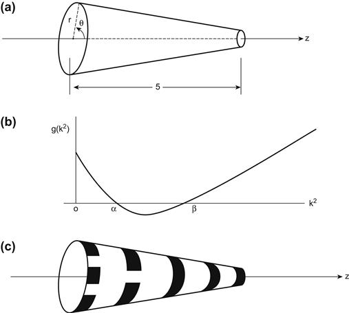
The constants d1, d2 are positive diffusion coefficients. A wealth of patterns may be revealed by these equations, depending on the geometry involved. Here we consider only the tapered cylindrical tail of the cat, which is approximated by a conical surface (Figure 11.3a). The molecular weight of U is considered to be higher than that of V, and so the diffusion coefficient d1 is smaller than d2. I want to show that if the thickness of the tail is small enough near its tip, then the only patterns that emerge are stripes. However, at the other end of the tail, near the rump, where the tail is thicker, it is possible for other patterns to appear. These conclusions are consonant with the observation of real animals (see Murray [87], Chs. 14 and 15).
The conical surface has an axial coordinate z, 0 ≤ z ≤ s, a radius r at location z, and an azimuthal coordinate θ. A position (x, y, z) on the surface is expressed in polar coordinates as (r cos θ, r sin θ, z), which gives rise to functions u(θ, z, t) and v(θ, z, t). Note that r is a fixed radius for each z, so r is not an independent variable.
I need to derive the Laplacian ∇2 = uxx + uyy + uzz in terms of the polar coordinates. This is accomplished in a manner similar to the way we derived ∇2 in Section 10.2, when r and θ were both independent variables, but it may be helpful to provide some details here.
First, ux = uθθx + uzzx = –uθ sin θ/r, since z is independent of x. Moreover, and for the same reason, uxx = (ux)θθx = θx(–uθθ sin θ/r – uθ cos θ/r) = uθθ sin2θ/r2 + uθ cos θ sin θ/r2.
In a similar manner, uyy = uθθ cos2θ/r2 – uθ cos θ sin θ/r2. It follows that
![]()
There is, of course, an identical expression for ∇2v.
We impose no-flux boundary conditions at the endpoints 0 and s of the cone, namely, that uz and vz both be zero. The need for these conditions is obvious at the narrow end of the cone, where the tail terminates (at z = s), whereas at z = 0 this is due to the fact that the rump end of the tail, near the animal’s underbelly, is where an unpigmented region begins. In addition, we require that any solution be periodic in θ.
Let u and v be spatially uniform and time-independent (namely, constant) solutions to (11.1). Linearize about this equilibrium solution by letting w be the column vector (u – u, v – v). Then
![]() (11.2)
(11.2)
where M is the Jacobean matrix of f, g evaluated at w = 0, namely, at u, v, and D is the diagonal matrix with entries d1 and d2.
A spatially independent solution to (11.2) satisfies wt = Mw, whose solutions are of the form ceλt, where λ is an eigenvalue of M and c is some vector multiple. This leads us to seek solutions to (11.2) that can be written as multiples of eλtW(θ, z). In the absence of any spatial variable but z, a time-independent solution w(z) that satisfies the no-flux conditions at z = 0 and z = s consists of multiples of cos kz, where k = nπ/s, in which case wzz = –k2w. This motivates us to seek a time-independent solution W to (11.2) that satisfies the eigenvalue problem
![]() (11.3)
(11.3)
for some scalar k. To see that eλtW actually solves (11.2), substitute it into this partial differential equation. The exponential term cancels out, and, because of (11.3), one finds that (M – k2D)W = λW, from which it follows that a nontrivial solution exists, provided that λ is an eigenvalue of the matrix M – k2D with corresponding eigenvector W. Note that λ depends on k2. When there is no spatial dependence, namely, k2 = 0, λ is then simply an eigenvalue of M.
To find W from (11.3) it suffices to separate variables. Let W(θ, z) = A(θ)B(z) to obtain two linear second-order and homogeneous ordinary differential equations for A and B. In particular, Bzz = –μ2B for some scalar μ > 0, and this has as solution B(z) = c1 cos μz + c2 sin μz. Applying our boundary conditions we get Bz(0) = 0, from which c2 = 0.
Also, Bz(s) = –c1μ sin μs = 0, from which μs = nπ, for n = 0, 1, 2, . . . . Hence, B(z) = c1 cos nπz/s.
As for A(θ), we require solutions periodic in θ, so we make the ansatz A(θ) = r cos mθ, for m = 1, 2, . . . .
Since (11.2) is linear, a solution can be generated as a superposition of functions of the form
![]() (11.4)
(11.4)
From (11.4) it is seen that Wzz = –(nπ/s)2W and Wθθ/r2 = –(m/r)2W, and (11.4) then establishes that
![]() (11.5)
(11.5)
Turing’s reaction–diffusion hypothesis is that any spatially uniform perturbation w(θ, z, t) of the equilibrium damps down to zero as t → ∝, and so spatial patterns can emerge only from initial perturbations that are not spatially uniform. Put another way, the uniform constant state is stable to all uniform disturbances, and patterns can appear only in the presence of diffusion. Since λ is to be an eigenvalue of M – k2D, namely, Det (M – k2D – λI) = 0, we see that in the absence of diffusion (k2 = 0), the stability of the constant state requires that Trace M < 0 and Det M > 0.
Now, Trace (M – k2D) < 0 for all nonzero k2, since the entries of the diagonal matrix k2D are positive. Therefore, to ensure that an initial perturbation of the constant state be unstable so that it will grow over time (a condition necessary for the onset of pattern formation), we must have g(k2) = Det (M – k2D) < 0.The function g(k2) is a quadratic in k2 given by
![]()
where m11 and m22 are the diagonal elements of M. Evidently the quadratic is positive when k2 = 0, and, since k4 eventually dominates as k2 increases, the quadratic is also positive for large k2. Therefore g(k2) becomes negative only if it crosses the k2-axis, which can happen only for some range of values 0 < α < k2 < β, as can be seen in Figure 11.3b.
It is clear that crossing the axis requires d1m22 + d2m11 to be positive (otherwise g(k2) is itself positive), and, since Trace M < 0, this means that d1 must necessarily be different than d2. However, we have assumed that d1 < d2 from the very beginning.
Using specific reaction terms, as given in Murray [87], it can be shown that g(k2) can indeed become negative for some range of values, and so, using (11.5), we obtain
![]() (11.6)
(11.6)
If r is below a certain critical value (at the thin end of the tail), then (11.6) is satisfied only for m = 0. Looking at (11.4), this means that the solutions are periodic in z, uniformly in θ, for some finite range of integer values n. This means that the concentration u alternates between peaks and troughs along the length of the tail, with coat markings that appear in the vicinity of every peak of u. This translates physically into a regular pattern of stripes.
When r is above the critical threshold, then (11.6) can be satisfied for a finite range of both m and n values. This means we are now along the thicker part of the tail, and the solutions are doubly periodic in this case, which implies that a genuinely two-dimensional pattern of spots will appear whenever the function peaks in value. Thus, there is a transition from two-dimensional coat markings to a one-dimensional set of stripes as we move along the tapered tail from rump to tip, as illustrated in Figure 11.3c.
This is what the linear theory indicates, but, of course, it cannot tell us how nonlinear system (11.1) actually evolves. What we have described here is only the onset of pattern formation. However, a numerical investigation of system (11.1) vindicates the conclusions drawn from the linear perturbation analysis (Murray [87,88]). In any event, the model is only a suggestive metaphor for what takes place in certain mammal hides. Moreover, these conclusions are very much dependent on the particular geometry of the animal’s body surface; it could be, for example, that no pattern appears anywhere.
11.3 Slime Molds
Let u(x, y, t) be the density of the single-cell amoeba and v(x, y, t) be the density of the attractant cAMP that is excreted by the amoeba. Recall the flow equation ρt = –qx of Section 10.1, which continues to be valid now, except that it is applied here to u and v separately in place of what was there identified with density ρ. The flow of amoebae is due to the normal motility of the individual cells of this organism, giving rise to a diffusion term with diffusivity μ. Additionally the amoebae move toward uneven concentrations of the attractant, which they release as the supply of bacteria on which they feed begins to be exhausted. This motion, known as chemotaxis, is proportional to cAMP gradients, namely, the rate of change of its spatial density. Since the attractant is released by the amoebae, the chemotaxis is proportional to u with some constant χ. Thus, the flow due to attraction is χu∇v, where, as usual, ∇v is the vector (ux, uy). Altogether, then, the one-dimensional term –qx is replaced by –∇q = –∇⋅(–μ∇u + χu∇v), with the plus sign indicating that chemotaxis is a movement toward the concentration of the gradient of v, and so the equation for u is
![]() (11.7)
(11.7)
As for v, there is also diffusive flux with diffusivity D plus a source term describing a simplified form of the kinetics. The growth of v is dependent on the concentration u, and there is a decay term for the dissipation of the attractant over time that is proportional to v. The kinetics is therefore given by fu – kv, with positive constants f and k. So the equation for v is
![]() (11.8)
(11.8)
At this juncture we imitate what was done for the Turing equations. Let u0, v0 be constant temporal-spatial homogeneous solutions of (11.7) and (11.8), and then linearize about this uniform solution by defining a column vector (u, v) = (u0 + u, v0 + v). Substituting w into the nonlinear equations and ignoring higher-order terms gives us a pair of linear equations:
![]() (11.9)
(11.9)
![]() (11.10)
(11.10)
in which it is assumed that fu0 – kv0 = 0. This is, of course, an unremarkable statement, since the pollution and decay of the attractant should balance in equilibrium.
Taking a cue from the way the Turing equations were treated in the previous section, let
![]() (11.11)
(11.11)
where c = (c1, c2). Basically, the form of the solution stems from the fact that the linear equations have solutions that can be Fourier synthesized by cosine terms or, equivalently, sine terms. Note that ∇2w = wxx + wyy = –2α2w, as can be verified directly. Therefore, substituting (11.11) into the two linearized equations gives us a system of algebraic equations Λc = σc, in which Λ is the matrix
![]()
The solution c = 0 corresponds to the steady-state equilibrium. In order for a growth pattern to emerge, it is therefore necessary that there be a nontrivial solution to Λc = σc, which forces the determinant of Λ to be zero. The determinant is a quadratic equation in σ, and its roots are given by
![]()
It is a tedious but straightforward computation to show that the two roots σ1 and σ2 are real and, since the sum of the roots is negative, namely,
![]()
the only way to ensure that solutions (11.11) do not dampen down to zero over time is that the two roots not both lie in the left half-plane, since this would imply that the equilibrium solution c = 0 is stable. To guarantee this to happen we need for the constant term to be negative, and this reduces to
![]() (11.12)
(11.12)
Can this be done? Begin by noting that α can be expressed as 2π/λ, where λ is the wavelength of the oscillatory solution to the linear system. If the wavelength is long enough—that is, if σ is sufficiently small, say, σ < σ0—and provided that
![]() (11.13)
(11.13)
then (11.12) is satisfied.
This threshold condition for instability is met if a suitable combination of the following conditions are satisfied: