Chapter 9
First‐order differentials and Jacobian matrices
1 INTRODUCTION
We begin this chapter with some notational issues. We shall strongly argue for a particular way of displaying the partial derivatives ∂fst(X)/∂xij of a matrix function F(X), one which generalizes the notion of a Jacobian matrix of a vector function to a Jacobian matrix of a matrix function.
For vector functions there is no controversy. Let f : S → ℝm be a vector function, defined on a set S in ℝn with values in ℝm. We have seen that if f is differentiable at a point x ∈ S, then its derivative Df(x) is an m × n matrix, also denoted by ∂f(x)/∂x′:
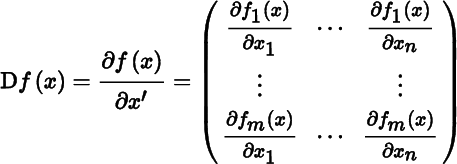
with, as a special case, for the scalar function ϕ (where m = 1):
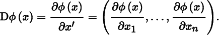
The notation ∂f(x)/∂x′ has the advantage of bringing out the dimension: we differentiate m elements of a column with respect to n elements of a row, and the result is an m × n matrix. This is just handy notation, it is not conceptual.
However, the fact that the partial derivatives ∂fs(x)/∂xi are organized in an m × n matrix and not, for example, in an n × m matrix or an mn‐vector is conceptual and it matters. All mathematics texts define vector derivatives in this way. There is no controversy about vector derivatives; there is, however, some controversy about matrix derivatives and this needs to be resolved.
The main tool in this chapter will be the first identification theorem (Theorem 5.11), which tells us how to obtain the derivative (Jacobian matrix) from the differential. Given a matrix function F(X), we then proceed as follows: (i) compute the differential of F(X), (ii) vectorize to obtain d vec F(X) = A(X) d vec X, and (iii) conclude that DF(X) = A(X). The simplicity and elegance of this approach will be demonstrated by many examples.
2 CLASSIFICATION
We shall consider scalar functions ϕ, vector functions f, and matrix functions F. Each of these may depend on one real variable ξ, a vector of real variables x, or a matrix of real variables X. We thus obtain the classification of functions and variables as shown in Table 9.1.
Table 9.1 Classification of functions and variables
| Scalar variable | Vector variable | Matrix variable | |
| Scalar function | ϕ(ξ) | ϕ(x) | ϕ(X) |
| Vector function | f(ξ) | f(x) | f(X) |
| Matrix function | F(ξ) | F(x) | F(X) |
To illustrate, consider the following examples:
| ϕ(ξ) | : | ξ2 |
| ϕ(x) | : | a′x, x′Ax |
| ϕ(X) | : | a′Xb, tr X′X, |X|, λ(X) (eigenvalue) |
| f(ξ) | : | (ξ, ξ2)′ |
| f(x) | : | Ax |
| f(X) | : | Xa, u(X) (eigenvector) |
| F(ξ) | : |  |
| F(x) | : | xx′ |
| F(X) | : | AXB, X2, X+. |
3 DERISATIVES
Now consider a matrix function F of a matrix of variables X; for example, F(X) = AXB or F(X) = X−1. How should we define the derivative of F? Surely this must be a matrix containing all the partial derivatives, but how? Some authors seem to believe that it does not matter, and employ the following ‘definition’:
Let F = (fst) be an m × p matrix function of an n × q matrix of variables X = (xij). Any r × c matrix A satisfying rc = mpnq and containing all the partial derivatives ∂fst(X)/∂xij is called a derisative of F.
In this ‘definition’, nothing is said about how the partial derivatives are organized in the matrix A. In order to distinguish this ‘definition’ from the correct definition (given in the next section), we shall call this concept a derisative and we shall use δ instead of ∂. (The word ‘derisative’ does not actually exist; it is introduced here based on the existing words derision, derisory, and derisive.)
In some textbooks in statistics and econometrics and in a number of papers, the derisative is recommended. For example, if F is a function of a scalar ξ, then one may define an expression
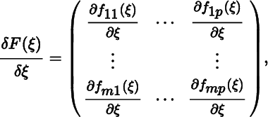
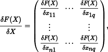
which has the same dimension as F. Based on (2), we may then define the derisative of a matrix with respect to a matrix as
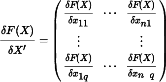
or as
or indeed in many other ways.
The derisative in (3) is of order mn × pq. In the special case where p = q = 1, we obtain the derisative of a vector f with respect to a vector x, and it is an mn × 1 column vector instead of an m × n matrix. Hence, this derisative does not have the usual vector derivative (1) as a special case.
The derisative in (4) is of order mq × np. Because of the transposition of the indexing, the derisative δf(x)/δx′ of a vector with respect to a vector is equal to the derivative Df(x) = ∂f(x)/∂x′. Hence, this derisative does have the vector derivative (1) as a special case.
Both derisatives share one rather worrying feature. If we look at the vector derivative (1), then we see that the ith row contains the partial derivatives of the ith function with respect to all variables, and the jth column contains the partial derivatives of all functions with respect to the jth variable. This is the key characteristic of the vector derivative, and it does not carry over to derisatives.
4 DERIVATIVES
If we wish to maintain this key characteristic in generalizing the concept of derivative, then we arrive at the following definition.
This is the only correct definition. The ordering of the functions and the ordering of the variables can be chosen freely. But any row of the derivative must contain the partial derivatives of one function only, and any column must contain the partial derivatives with respect to one variable only. Any matrix containing all partial derivatives and satisfying this requirement is a derivative; any matrix containing all partial derivatives and not satisfying this requirement is not a derivative; it is a derisative.
To obtain the derivative, we need to stack the elements of the function F and also the elements of the argument matrix X. Since the vec operator is the commonly used stacking operator, we use the vec operator. There exist other stacking operators (for example, by organizing the elements row‐by‐row rather than column‐by‐column), and these could be used equally well as long as this is done consistently. A form of stacking, however, is essential in order to preserve the notion of derivative. We note in passing that all stacking operations are in one‐to‐one correspondence with each other and connected through permutation matrices. For example, the row‐by‐row and column‐by‐column stacking operations are connected through the commutation matrix. There is therefore little advantage in developing the theory of matrix calculus for more than one stacking operation.
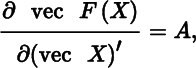
Thus motivated, we define the matrix derivative as
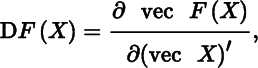
which is an mp × nq matrix. The definition of vector derivative (p = q = 1) is a special case of the more general definition of matrix derivative, as of course it should. The definition implies that, if F is a function of a scalar ξ(n = q = 1), then DF(ξ) = ∂ vec F(ξ)/∂ξ, a column mp‐vector. Also, if ϕ is a scalar function of a matrix X (m = p = 1), then Dϕ(X) = ∂ϕ(X)/∂(vec X)′, a 1 × nq row vector.
The choice of ordering the partial derivatives is not arbitrary. For example, the derivative of the scalar function ϕ(X) = tr(X) is not Dϕ(X) = In (as is often stated), but Dϕ(X) = (vec In)′.
The use of a correct notion of derivative matters. A generalization should capture the essence of the concept to be generalized. For example, if we generalize the concept of the reciprocal b = 1/a from a scalar a to a matrix A, we could define a matrix B whose components are bij = 1/aij. But somehow this does not capture the essence of reciprocal, which is ab = ba = 1. Hence, we define B to satisfy AB = BA = I. The elements of the matrix B = A−1 are not ordered arbitrarily. The inverse is more than a collection of its elements; it is a higher‐dimensional unit with a meaning.
Similarly, if we generalize the univariate normal distribution to a ‘matrix‐variate’ normal distribution, how should we proceed? Surely we want to use the fact that there already exists a multivariate (vector‐variate) normal distribution, and that this is an established part of statistics. The matrix‐variate normal distribution should be a generalization of the vector‐variate normal distribution. For example, it would be unacceptable if the variance matrix of the matrix‐variate distribution would not be symmetric or if each row and each column of the variance matrix would not contain all covariances between one variate and all other variates. Such an arrangement would not generalize the well‐established vector‐variate distribution to the matrix‐variate distribution, and hence would place itself outside mainstream statistics.
Finally, suppose we consider a set of transformations
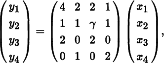
or, for short, y = Ax, where γ is left free for the moment. The Jacobian of this transformation is the absolute value of the determinant of the derivative, here |∂y/∂x′| = |A| = 6γ − 2. Now suppose we organize x and y into 2 × 2 matrices, such that x = vec X and y = vec Y. So, instead of (x1, x2, x3, x4), we consider (x11, x21, x12, x22) and the same for y. What is now the Jacobian of the transformation from the 2 × 2 matrix X to the 2 × 2 matrix Y = F(X)? The trivial relabeling should not affect the Jacobian. Since
the Jacobian of the transformation is still |A| = 6γ − 2. Notice that if we organize the four functions in a different way, for example as (x11, x12, x21, x22), then the sign of the determinant may change, but not its absolute value. Hence, relabeling does not affect the Jacobian (when using derivatives; but it does when we use derisatives!)
In summary, there exists a well‐established theory of vector derivatives, and we want to define matrix derivatives within this established theory. The eminent mathematicians who contributed to vector calculus realized not only that the possibility to approximate a given function by means of an affine function is the key property of differentiability, but they also realized that in this framework trivial changes such as relabeling functions or variables has only trivial consequences for the derivative: rows and columns are permuted, but the rank is unchanged and the determinant (in the case of a square matrix) is also unchanged (apart possibly from its sign). This is what the derivative achieves and what the derisative does not achieve. The arrangement of the partial derivatives matters because a derivative is more than just a collection of partial derivatives. It is a mathematical concept, a mathematical unit, just like the inverse or the variance of the multivariate normal distribution.
From a theoretical point of view, derisatives do not generalize the concept of vector derivative to matrix derivative and hence do not allow us to interpret the rank of the derivative or its determinant. But also from a practical point of view there are no advantages in using derisatives. It is true that we can obtain a product rule and a chain rule for the various derisatives, but these are more complicated and less easy to use than the product and chain rules for derivatives. It seems then that there are only advantages, and not a single disadvantage, for using the concept of derivative, as we shall illustrate further in the following sections.
5 IDENTIFICATION OF JACOBIAN MATRICES
Our strategy to find the Jacobian matrix of a function will not be to evaluate each of its partial derivatives, but rather to find the differential. In the case of a differentiable vector function f(x), the first identification theorem (Theorem 5.6) tells us that there exists a one‐to‐one correspondence between the differential of f and its Jacobian matrix. More specifically, it states that
implies and is implied by
Thus, once we know the differential, the Jacobian matrix is identified.
The extension to matrix functions is straightforward. The identification theorem for matrix functions (Theorem 5.11) states that
implies and is implied by
Since computations with differentials are relatively easy, this identification result is extremely useful. Given a matrix function F(X), we may therefore proceed as follows: (i) compute the differential of F(X), (ii) vectorize to obtain d vec F(X) = A(X) d vec X, and (iii) conclude that DF(X) = A(X).
Many examples in this chapter will demonstrate the simplicity and elegance of this approach. Let us consider one now. Let F(X) = AXB, where A and B are matrices of constants. Then,
and
so that
6 THE FIRST IDENTIFICATION TABLE
The identification theorem for matrix functions of matrix variables encompasses, of course, identification for matrix, vector, and scalar functions of matrix, vector, and scalar variables. Table 9.2 lists these results.
Table 9.2 The first identification table
| Function | Differential | Derivative/Jacobian | Order of D |
| ϕ(ξ) | dϕ = αdξ |
Dϕ(ξ) = α |
1 × 1 |
| ϕ(x) | dϕ = a′dx |
Dϕ(x) = a′ |
1 × n |
| ϕ(X) | 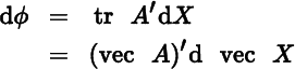 |
Dϕ(X) = (vec A)′ |
1 × nq |
| f(ξ) | df = a dξ |
Df(ξ) = a |
m × 1 |
| f(x) | df = A dx |
Df(x) = A |
m × n |
| f(X) | df = A d vec X |
Df(X) = A |
m × nq |
| F(ξ) | dF = A dξ |
DF(ξ) = vec A |
mp × 1 |
| F(x) | d vec F = A dx |
DF(x) = A |
mp × n |
| F(X) | d vec F = A d vec X |
DF(X) = A |
mp × nq |
In this table, ϕ is a scalar function, f an m × 1 vector function, and F an m × p matrix function; ξ is a scalar, x an n × 1 vector, and X an n × q matrix; α is a scalar, a is a column vector, and A is a matrix, each of which may be a function of X, x, or ξ.
7 PARTITIONING OF THE DERIVATIVE
Before the workings of the identification table are exemplified, we have to settle one further question of notation. Let ϕ be a differentiable scalar function of an n × 1 vector x. Suppose that x is partitioned as
Then the derivative Dϕ(x) is partitioned in the same way, and we write
where D1ϕ(x) contains the partial derivatives of ϕ with respect to x1, and D2ϕ(X) contains the partial derivatives of ϕ with respect to x2. As a result, if
then
and so
8 SCALAR FUNCTIONS OF A SCALAR
It seems trivial to consider scalar functions of a scalar, but sometimes the function depends on a matrix, which depends on a scalar. Let us give one example. Consider the function
where Y = Y(ξ) is a function of a scalar ξ. Taking the differential gives
and hence
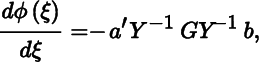
where G = (gij) is the matrix whose ijth element is given by gij = dYij/dξ.
9 SCALAR FUNCTIONS OF A VECTOR
The two most important cases of a scalar function of a vector x are the linear form a′x and the quadratic form x′Ax.
Let ϕ(x) = a′x, where a is a vector of constants. Then dϕ(x) = a′dx, so Dϕ(x) = a′. Next, let ϕ(x) = x′Ax, where A is a square matrix of constants. Then,
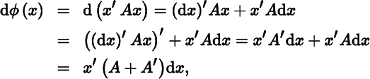
so that Dϕ(x) = x′(A + A′). Thus, we obtain Table 9.3.
Table 9.3 Differentials of linear and quadratic forms
| ϕ(x) | dϕ(x) |
Dϕ(x) |
Condition |
| a′x | a′dx |
a′ | |
| x′Ax | x′(A + A′) dx |
x′(A + A′) | |
| x′Ax | 2x′A dx |
2x′A | A symmetric |
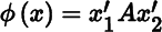
A little more complicated is the situation where ϕ is a scalar function of a matrix, which in turn is a function of vector. For example, let
Letting
we obtain
and hence
Exercises
- 1.
If ϕ(x) = a′f(x), then
Dϕ(x) = a′Df(x). - 2.
If ϕ(x) = (f(x))′g(x), then
Dϕ(x) = (g(x))′Df(x) + (f(x))′Dg(x). - 3.
If ϕ(x) = x′Af(x), then
Dϕ(x) = (f(x))′A′ + x′ADf(x). - 4.
If ϕ(x) = (f(x))′Af(x), then
Dϕ(x) = (f(x))′(A + A′)Df(x). - 5.
If ϕ(x) = (f(x))′Ag(x), then
Dϕ(x) = (g(x))′A′Df(x)+(f(x))′ADg(x). - 6. If
 , where
 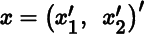 , then
  , and
, and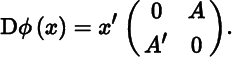
10 SCALAR FUNCTIONS OF A MATRIX, I: TRACE
There is no lack of interesting examples of scalar functions of matrices. In this section, we shall investigate differentials of traces of some matrix functions. Section 9.11 is devoted to determinants and Section 9.12 to eigenvalues.
The simplest case is
implying
More interesting is the trace of the (positive semidefinite) matrix function X′X. We have
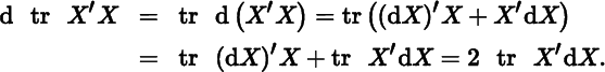
Hence,
Next consider the trace of X2, where X is square. This gives
and thus
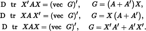
In Table 9.4, we present straightforward generalizations of the three cases just considered. The proofs are easy and are left to the reader.
Table 9.4 Differentials involving the trace
| ϕ(X) | dϕ(X) |
Dϕ(X) |
G |
| tr AX | tr A dX |
(vec G)′ | A′ |
| tr XAX′B | tr(AX′B + A′X′B′)dX |
(vec G)′ | B′XA′ + BXA |
| tr XAXB | tr(AXB + BXA)dX |
(vec G)′ | B′X′A′ + A′X′B′ |
Exercises
- 1. Show that tr BX′, tr XB, tr X′B, trBXC, and tr BX′C can all be written as tr AX and determine their derivatives.
- 2.
Show that
- 3.
Show that

- 4. Use the previous results to find the derivatives of a′Xb, a′XX′a, and a′X−1a.
- 5.
Show that for square X,

- 6.
If ϕ(X) = tr F(X), then
Dϕ(X) = (vec I)′DF(X). - 7. Determine the derivative of ϕ(X) = tr F(X)AG(X)B.
- 8. Determine the derivative of ϕ(X, Z) = tr AXBZ.
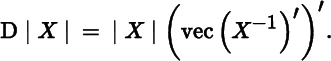
11 SCALAR FUNCTIONS OF A MATRIX, II: DETERMINANT
Recall from Theorem 8.1 that the differential of a determinant is given by
if X is a square nonsingular matrix. As a result, the derivative is
Let us now employ Equation (5) to find the differential and derivative of the determinant of some simple matrix functions of X. The first of these is |XX′|, where X is not necessarily a square matrix, but must have full row rank in order to ensure that the determinant is nonzero (in fact, positive). The differential is
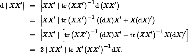
As a result,
![]()
Similarly we find for |X′X| ≠ 0,
so that
Finally, let us consider the determinant of X2, where X is nonsingular. Since |X2| = |X|2, we have
and
These results are summarized in Table 9.5, where each determinant is assumed to be nonzero.
Table 9.5 Differentials involving the determinant
| ϕ(x) | dϕ(X) |
Dϕ(X) |
G |
| |X| | |X| tr X−1dX |
(vec G)′ | |X|(X−1)′ |
| |XX′| | 2|XX′| tr X′(XX′)−1dX |
(vec G)′ | 2|XX′|(XX′)−1X |
| |X′X| | 2|X′X| tr(X′X)−1X′dX |
(vec G)′ | 2|X′X|X(X′X)−1 |
| |X2| | 2|X|2 tr X−1dX |
(vec G)′ | 2|X|2(X−1)′ |
Exercises
- 1.
Show that
D|AXB| = (vec G)′ with G = |AXB|A′(B′X′A′)−1B′, if the inverse exists. - 2.
Let F(X) be a square nonsingular matrix function of X, and Z(X) = C(F(X))−1A. Then,
D|F(X)| = (vec G)′, where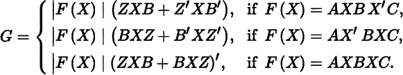
- 3.
Generalize (5) and (8) for nonsingular X to
D|Xp| = (vec G)′, where G = p|X|p(X′)−1, a formula that holds for positive and negative integers. - 4. Determine the derivative of ϕ(X) = log |X′AX|, where A is positive definite and X′AX nonsingular.
- 5. Determine the derivative of ϕ(X) = |AF(X)BG(X)C|, and verify (6), (7), and (8) as special cases.
12 SCALAR FUNCTIONS OF A MATRIX, III: EIGENVALUE
Let X0 be a symmetric n × n matrix, and let u0 be a normalized eigenvector associated with a simple eigenvalue λ0 of X0. Then we know from Section 8.9 that unique and differentiable functions λ = λ(X) and u = u(X) exist for all X in a neighborhood N(X0) of X0 satisfying
and
The differential of λ at X0 is then
Hence, we obtain the derivative
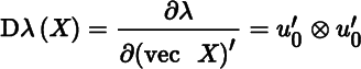
and the gradient (a column vector!)
13 TWO EXAMPLES OF VECTOR FUNCTIONS
Let us consider a set of variables y1, …, ym, and suppose that these are known linear combinations of another set of variables x1, …, xn, so that
Then,
and since df(x) = Adx, we have for the Jacobian matrix
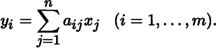
If, on the other hand, the yi are linearly related to variables xij such that
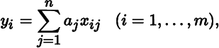
then this defines a vector function
The differential in this case is
and we find for the Jacobian matrix
Exercises
- 1.
Show that the Jacobian matrix of the vector function f(x) = Ag(x) is
Df(x) = ADg(x), and generalize this to the case where A is a matrix function of x. - 2.
Show that the Jacobian matrix of the vector function f(x) = (x′x)a is
Df(x) = 2ax′, and generalize this to the case where a is a vector function of x. - 3. Determine the Jacobian matrix of the vector function f(x) = ∇ϕ(x). This matrix is, of course, the Hessian matrix of ϕ.
- 4.
Show that the Jacobian matrix of the vector function f(X) = X′a is
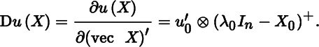
Df(X) = In ⊗ a′ when X has n columns. - 5. Under the conditions of Section 9.12, show that the derivative at X0 of the eigenvector function u(X) is given by
14 MATRIX FUNCTIONS
An example of a matrix function of an n × 1 vector of variables x is
The differential is
so that
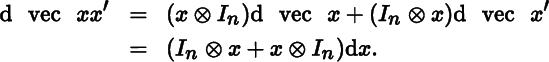
Hence,
Next, we consider four simple examples of matrix functions of a matrix or variables X, where the order of X is n × q. First the identity function
Clearly, d vec F(X) = d vec X, so that
More interesting is the transpose function
We obtain
Hence,
The commutation matrix K is likely to play a role whenever the transpose of a matrix of variables occurs. For example,
so that
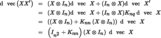
and
where ![]() is the symmetric idempotent matrix defined in Theorem 3.11. In a similar fashion, we obtain
is the symmetric idempotent matrix defined in Theorem 3.11. In a similar fashion, we obtain
so that
These results are summarized in Table 9.6, where X is an n × q matrix of variables.
Table 9.6 Simple matrix differentials
| F(X) | dF(X) |
DF(X) |
| X | dX |
Inq |
| X′ | (dX)′ |
Knq |
| XX′ | (dX)X′ + X(dX)′ |
2Nn(X ⊗ In) |
| X′X | (dX)′X + X′dX |
2Nq(Iq ⊗ X′) |
If X is a nonsingular n × n matrix, then
Taking vecs we obtain
and hence
Finally, if X is square then, for p = 1, 2, …,
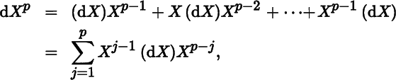
so that
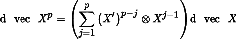
and
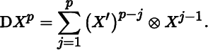
The last two examples are summarized in Table 9.7.
Table 9.7 Matrix differentials involving powers
| F(X) | dF(X) |
DF(X) |
Conditions |
| X−1 | −X−1(dX)X−1 |
−(X′)−1 ⊗ X−1 | X nonsingular |
| Xp | X square |
Exercises
- 1. Find the Jacobian matrix of the matrix functions AXB and AX−1 B.
- 2. Find the Jacobian matrix of the matrix functions XAX′, X′AX, XAX, and X′AX′.
- 3. What is the Jacobian matrix of the Moore‐Penrose inverse F(X) = X+ (see Section 8.5).
- 4. What is the Jacobian matrix of the adjoint matrix F(X) = X# (see Section 8.6).
- 5. Let F(X) = AH(X)BZ(X)C, where A, B, and C are constant matrices. Find the Jacobian matrix of F.
- 6. (product rule) Let F (m × p) and G (p × r) be functions of X (n × q). From the product rule for differentials
d(FG) = (dF)G + F(dG), apply the vec operator, and show that
15 KRONECKER PRODUCTS
An interesting problem arises in the treatment of Kronecker products. Consider the matrix function
The differential is easily found as
and, on taking vecs, we obtain
In order to find the Jacobian of F, we must find matrices A(Y) and B(X) such that
and
in which case the Jacobian matrix of F(X, Y) takes the partitioned form
The crucial step here is to realize that we can express the vec of a Kronecker product of two matrices in terms of the Kronecker product of their vecs, that is
where it is assumed that X is an n × q matrix and Y is a p × r matrix (see Theorem 3.10).
Using (9), we now write
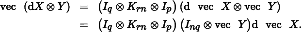
Hence,
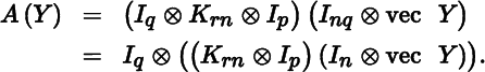
In a similar fashion we find
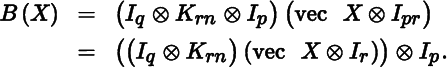
We thus obtain the useful formula
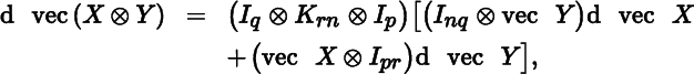
from which the Jacobian matrix of the matrix function F(X, Y) = X ⊗ Y follows:
Exercises
- 1. Let F(X, Y) = XX′ ⊗YY′, where X has n rows and Y has p rows (the number of columns of X and Y is irrelevant). Show that

where
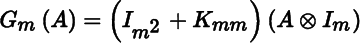
for any matrix A having m rows. Compute
DF(X, Y). - 2. Find the differential and the derivative of the matrix function F(X, Y) = X ⊙ Y (Hadamard product).
16 SOME OTHER PROBLEMS
Suppose we want to find the Jacobian matrix of the real‐valued function ϕ : ℝn × q → ℝ given by
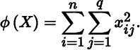
We can, of course, obtain the Jacobian matrix by first calculating (easy, in this case) the partial derivatives. More appealing, however, is to note that
from which we obtain
and
This example is, of course, very simple. But the idea of expressing a function of X in terms of the matrix X rather than in terms of the elements xij is often important. Three more examples should clarify this.
Let ϕ(X) be defined as the sum of the n2 elements of X−1. Then, let ı = (1, 1, …, 1)′ of order n × 1 and write
from which we easily obtain
and hence
Consider another example. Let F(X) be the n × (n − 1) matrix function of an n × n matrix of variables X defined as X−1 without its last column. Then, let En be the n × (n − 1) matrix obtained from the identity matrix In by deleting its last column, i.e.
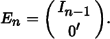
With En so defined, we can express F(X) as
It is then simple to find
and hence
As a final example, consider the real‐valued function ϕ(X) defined as the ijth element of X2. In this case, we can write
where ei and ej are elementary vectors. Hence,
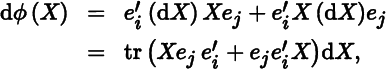
so that
17 JACOBIANS OF TRANSFORMATIONS
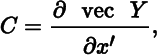
If Y is a one‐to‐one function of X, then the matrix
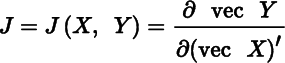
is the Jacobian matrix of the transformation from X to Y, and the absolute value of its determinant |J| is called the Jacobian of the transformation.
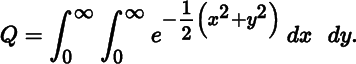
The Jacobian plays a role in changing variables in multiple integrals. For example, suppose we wish to calculate
Making the change of variables
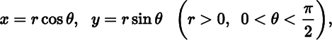
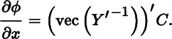
we obtain
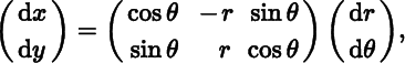
so that the Jacobian is given by
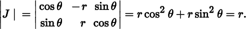
Then, using the fact that ![]() , we find
, we find

This, by the way, implies that ![]() ,thus showing that the standard‐normal density integrates to one.
,thus showing that the standard‐normal density integrates to one.
Its determinant is |J| = (−1)2 |X|−2n, using Equation (9) in Chapter 2, and hence the Jacobian of the transformation is |X|−2n.
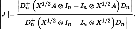
Jacobians often involve symmetric matrices or, more generally, matrices that satisfy a given set of linear restrictions. This is where the duplication matrix comes in, as the following example shows.
Since both X1/2 and Y are symmetric, we can write
In particular, for A = In, we have Y = X and hence
The required Jacobian is thus the absolute value of
BIBLIOGRAPHICAL NOTES
3. See also Magnus and Neudecker (1985) and Pollock (1985). The derisative in (3) is advocated, inter alia, by Graham (1981) and Boik (2008).
4. The point in this section has been made before; see Neudecker (1969), Pollock (1979, 1985), Magnus and Neudecker (1985), Abadir and Magnus (2005), and Magnus (2010).
17. Jacobians are treated extensively in Magnus (1988, Chapter 8), where special attention is given to symmetry and other so‐called linear structures; see also Mathai (1997). Exercise 2 is Theorem 8.1(iv) from Magnus (1988).