Chapter 8
Some important differentials
1 INTRODUCTION
Now that we know what differentials are and have adopted a convenient and simple notation for them our next step is to determine the differentials of some important functions. We shall discuss the differentials of some scalar functions of X (eigenvalue, determinant), a vector function of X (eigenvector), and some matrix functions of X (inverse, Moore‐Penrose (MP) inverse, adjoint matrix).
But first, we must list the basic rules.
2 FUNDAMENTAL RULES OF DIFFERENTIAL CALCULUS
The following rules are easily verified. If u and v are real‐valued differentiable functions and α is a real constant, then we have
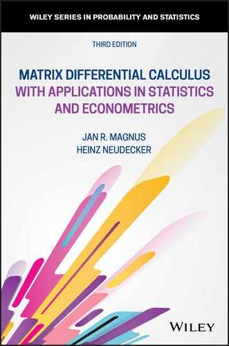
and also
The differential of the power function is
where the domain of definition of the power function uα depends on the arithmetical nature of α. If α is a positive integer, then uα is defined for all real u; but if α is a negative integer or zero, the point u = 0 must be excluded. If α is a rational fraction, e.g. α = p/q (where p and q are integers and we can always assume that q > 0), then ![]() , so that the function is determined for all values of u when q is odd, and only for u ≥ 0 when q is even. In cases where α is irrational, the function is defined for u > 0.
, so that the function is determined for all values of u when q is odd, and only for u ≥ 0 when q is even. In cases where α is irrational, the function is defined for u > 0.
The differentials of the logarithmic and exponential functions are
Similar results hold when U and V are matrix functions, and A is a matrix of real constants:
For the Kronecker product and Hadamard product, the analog of (13) holds:
Finally, we have
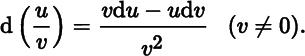
For example, to prove (3), let ϕ(x) = u(x) + v(x). Then,
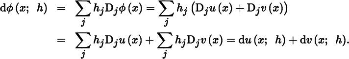
As a second example, let us prove ( 13 ). Using only ( 3 ) and (4), we have
Exercises
- 1. Prove Equation (14).
- 2. Show that d(UVW) = (dU)VW + U(dV)W + UV(dW).
- 3. Show that d(AXB) = A(dX)B, where A and B are constant.
- 4. Show that d tr X′X = 2 tr X′dX.
- 5. Let u : S → ℝ be a real‐valued function defined on an open subset S of ℝn. If u′u = 1 on S, then u′du = 0 on S.
3 THE DIFFERENTIAL OF A DETERMINANT
Let us now apply these rules to obtain a number of useful results. The first of these is the differential of the determinant.
It is worth stressing that at points where r(F(X)) = m − 1, F(X) must have at least one zero eigenvalue. At points where F(X) has a simple zero eigenvalue (and where, consequently, r(F(X)) = m − 1), (20) simplifies to
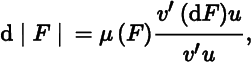
where μ(F(X)) is the product of the m − 1 nonzero eigenvalues of F(X).
In the previous proof, we needed element‐by‐element differentiation, something that we would rather avoid. Hence, let us provide a second proof, which is closer to the spirit of matrix differentiation.
We do not, at this point, derive the second‐ and higher‐order differentials of the determinant function. In Section 8.4 (Exercises 1 and 2), we obtain the differentials of log |F| assuming that F(X) is nonsingular. To obtain the general result, we need the differential of the adjoint matrix. A formula for the first differential of the adjoint matrix will be obtained in Section 8.6.
Result ( 19 ), the case where F(X) is nonsingular, is of great practical interest. At points where |F(X)| is positive, its logarithm exists and we arrive at the following theorem.
Exercises
- 1. Give an intuitive explanation of the fact that d|X| = 0 at points X ∈ ℝn × n, where r(X) ≤ n − 2.
- 2. Show that, if F(X) ∈ ℝm × m and r(F(X)) = m − 1 for every X in some neighborhood of X0, then d|F(X)| = 0 at X0.
- 3. Show that d log |X′X| = 2 tr(X′X)−1 X′dX at every point where X has full column rank.
4 THE DIFFERENTIAL OF AN INVERSE
The next theorem deals with the differential of the inverse function.
Let us consider the set T of nonsingular real m × m matrices. T is an open subset of ℝm × m, so that for every Y0 ∈ T, there exists an open neighborhood N(Y0) all of whose points are nonsingular. This follows from the continuity of the determinant function |Y|. Put differently, if Y0 is nonsingular and {Ej} is a sequence of real m × m matrices such that Ej → 0 as j → ∞, then
for every j greater than some fixed j0, and
Exercises
- 1. Let T+ = {Y : Y ∈ ℝm × m, ∣ Y ∣ > 0}. If F : S → T+, S ⊂ ℝn × q, is twice differentiable on S, then show that
d2 log ∣ F ∣ = − tr(F−1dF)2 + tr F−1d2F.
- 2. Show that, for X ∈ T+, log |X| is ∞ times differentiable on T+, and

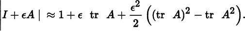
- 3. Let ϕ(ɛ) = log |I + ɛA|. Show that the rth derivative of ϕ evaluated at ɛ = 0 is given by

- 4. Hence, we have the following approximation for small ɛ:
(Compare Exercises 2 and 3 in Section 1.13.)
- 5. Let T = {Y : Y ∈ ℝm × m, ∣ Y ∣ ≠ 0}. If F : S → T, S ⊂ ℝn × q, is twice differentiable on S, then show
d2F−1 = 2[F−1(dF)]2F−1 − F−1(d2F)F−1.
- 6. Show that, for X ∈ T, X−1 is ∞ times differentiable on T, and

5 DIFFERENTIAL OF THE MOORE‐PENROSE INVERSE
Equation (26) above and Exercise 1 in Section 5.15 tell us that nonsingular matrices have locally constant rank. Singular matrices (more precisely matrices of less than full row and column rank) do not share this property. Consider, for example, the matrices
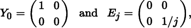
and let Y = Y(j) = Y0 + Ej. Then r(Y0) = 1, but r(Y) = 2 for all j. Moreover, Y → Y0 as j → ∞, but
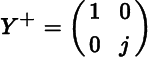
does not converge to ![]() , because it does not converge to anything. It follows that (i) r(Y) is not constant in any neighborhood of Y0 and (ii) Y+ is not continuous at Y0. The following proposition shows that the conjoint occurrence of (i) and (ii) is typical.
, because it does not converge to anything. It follows that (i) r(Y) is not constant in any neighborhood of Y0 and (ii) Y+ is not continuous at Y0. The following proposition shows that the conjoint occurrence of (i) and (ii) is typical.
We now have all the ingredients for the main result.
Exercises
- 1. Prove (28).
- 2. If F(X) is idempotent for every X in some neighborhood of a point X0, then F is said to be locally idempotent at X0. Show that F(dF)F = 0 at points where F is differentiable and locally idempotent.
- 3. If F is locally idempotent at X0 and continuous in a neighborhood of X0, then tr F is differentiable at X0 with d(tr F)(X0) = 0.
- 4. If F has locally constant rank at X0 and is continuous in a neighborhood of X0, then tr F+ F and tr FF+ are differentiable at X0 with d(tr F+F)(X0) = d(tr FF+)(X0) = 0.
- 5. If F has locally constant rank at X0 and is differentiable in a neighborhood of X0, then tr FdF+ = −trF+dF.
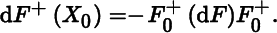
6 THE DIFFERENTIAL OF THE ADJOINT MATRIX
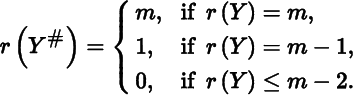
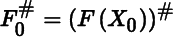
If Y is a real m × m matrix, then by Y# we denote the m × m adjoint matrix of Y. Given an m × m matrix function F, we now define an m × m matrix function F# by F#(X) = (F(X))#. The purpose of this section is to find the differential of F#. We first prove Theorem 8.6.
Recall from Theorem 3.2 that if Y = F(X) is an m × m matrix and m ≥ 2, then the rank of Y# = F#(X) is given by
As a result, two special cases of Theorem 8.6 can be proved. The first relates to the situation where F(X0) is nonsingular.
The second special case of Theorem 8.6 concerns points where the rank of F(X0) does not exceed m − 3.
There is another, more illuminating, proof of Corollary 8.2 — one which does not depend on Theorem 8.6. Let Y0 ∈ ℝm × m and assume Y0 is singular. Then r(Y) is not locally constant at Y0. In fact, if r(Y0) = r (1 ≤ r ≤ m − 1) and we perturb one element of Y0, then the rank of ![]() (the perturbed matrix) will be r − 1, r, or r + 1. An immediate consequence of this simple observation is that if r(Y0) does not exceed m − 3, then
(the perturbed matrix) will be r − 1, r, or r + 1. An immediate consequence of this simple observation is that if r(Y0) does not exceed m − 3, then ![]() will not exceed m − 2. But this means that at points Y0 with r(Y0) ≤ m − 3,
will not exceed m − 2. But this means that at points Y0 with r(Y0) ≤ m − 3,
implying that the differential of Y# at Y0 must be the null matrix.
These two corollaries provide expressions for dF# at every point X where r(F(X)) = m or r(F(X)) ≤ m − 3. The remaining points to consider are those where r(F(X)) is either m − 1 or m − 2. At such points we must unfortunately use Theorem 8.6, which holds irrespective of rank considerations.
Only if we know that the rank of F(X) is locally constant can we say more. If r(F(X)) = m − 2 for every X in some neighborhood N(X0) of X0, then F#(X) vanishes in that neighborhood, and hence (dF#)(X) = 0 for every X ∈ N(X0). More complicated is the situation where r(F(X)) = m − 1 in some neighborhood of X0. A discussion of this case is postponed to Miscellaneous Exercise 7 at the end of this chapter.
Exercise
- 1. The matrix function F : ℝn × n → ℝn × n defined by F(X) = X# is ∞ times differentiable on ℝn × n, and (djF)(X) = 0 for every j ≤ n − 2 − r(X).
7 ON DIFFERENTIATING EIGENVALUES AND EIGENVECTORS
There are two problems involved in differentiating eigenvalues and eigenvectors. The first problem is that the eigenvalues of a real matrix A need not, in general, be real numbers — they may be complex. The second problem is the possible occurrence of multiple eigenvalues.
To appreciate the first point, consider the real 2 × 2 matrix function
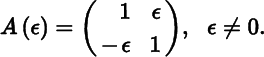
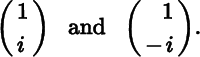
The matrix A is not symmetric, and its eigenvalues are 1 ± iɛ. Since both eigenvalues are complex, the corresponding eigenvectors must be complex as well; in fact, they can be chosen as
We know, however, from Theorem 1.4 that if A is a symmetric matrix, then its eigenvalues are real and its eigenvectors can always be taken to be real. Since the derivations in the symmetric case are somewhat simpler, we shall only consider the symmetric case.
Thus, let X0 be a symmetric n × n matrix, and let u0 be a (normalized) eigenvector associated with an eigenvalue λ0 of X0, so that the triple (X0, u0, λ0) satisfies the equations
Since the n + 1 equations in (35) are implicit relations rather than explicit functions, we must first show that there exist explicit unique functions λ = λ(X) and u = u(X) satisfying ( 35 ) in a neighborhood of X0 and such that λ(X0) = λ0 and u(X0) = u0. Here, the second (and more serious) problem arises: the possible occurrence of multiple eigenvalues.
We shall see that the implicit function theorem (given in the Appendix to Chapter 7) implies the existence of a neighborhood N(X0) ⊂ ℝn × n of X0, We shall see that the implicit function theorem (given in the Appendix to Chapter 7) implies the existence of a neighborhood N(X0) ⊂ ℝn × n of X0, where the functions λ and u both exist and are ∞ times (continuously) differentiable, provided λ0 is a simple eigenvalue of X0. If, however, λ0 is a multiple eigenvalue of X0, then the conditions of the implicit function theorem are not satisfied. The difficulty is illustrated by the real 2 × 2 matrix function
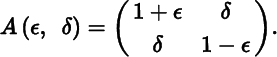
The matrix A is symmetric for every value of ɛ and δ; its eigenvalues are ![]() and
and ![]() . Both eigenvalue functions are continuous in ɛ and δ, but clearly not differentiable at (0, 0). (Strictly speaking, we should also prove that λ1 and λ2 are the only two continuous eigenvalue functions.) The conical surface formed by the eigenvalues of A(ɛ, δ) has a singularity at ɛ = δ = 0 (Figure 8.1). For a fixed ratio ɛ/δ however, we can pass from one side of the surface to the other going through (0, 0) without noticing the singularity. This phenomenon is quite general and it indicates the need to restrict our study of differentiability of multiple eigenvalues to one‐dimensional perturbations only.
. Both eigenvalue functions are continuous in ɛ and δ, but clearly not differentiable at (0, 0). (Strictly speaking, we should also prove that λ1 and λ2 are the only two continuous eigenvalue functions.) The conical surface formed by the eigenvalues of A(ɛ, δ) has a singularity at ɛ = δ = 0 (Figure 8.1). For a fixed ratio ɛ/δ however, we can pass from one side of the surface to the other going through (0, 0) without noticing the singularity. This phenomenon is quite general and it indicates the need to restrict our study of differentiability of multiple eigenvalues to one‐dimensional perturbations only.
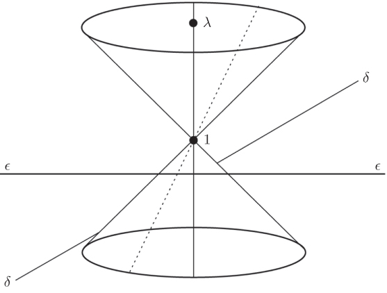
Figure 8.1 The eigenvalue functions 
8 THE CONTINUITY OF EIGENPROJECTIONS
When employing arguments that require limits such as continuity or consistency, some care is required when dealing with eigenvectors and associated concepts.
We shall confine ourselves to an n × n symmetric (hence real) matrix, say A. If Ax = λx for some x ≠ 0, then λ is an eigenvalue of A and x is an eigenvector of A associated with λ. Because of the symmetry of A, all its eigenvalues are real and they are uniquely determined (Theorem 1.4). However, eigenvectors are not uniquely determined, not even when the eigenvalue is simple. Also, while the eigenvalues are typically continuous functions of the elements of the matrix, this is not necessarily so for the eigenvectors.
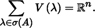
Some definitions are required. The set of all eigenvalues of A is called its spectrum and is denoted by σ(A). The eigenspace of A associated with λ is
The dimension of V(λ) is equal to the multiplicity of λ, say m(λ). Eigenspaces associated with distinct eigenvalues are orthogonal to each other. Because of the symmetry of A, we have the decomposition
The eigenprojection of A associated with λ of multiplicity m(λ), denoted by P(λ), is given by the symmetric idempotent matrix
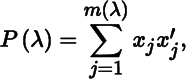
where the {xj} form any set of m orthonormal vectors in V(λ), that is, ![]() and
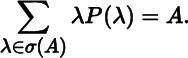
and ![]() for i ≠ j. While eigenvectors are not unique, the eigenprojection is unique because an idempotent matrix is uniquely determined by its range and null space. The spectral decomposition of A is then
for i ≠ j. While eigenvectors are not unique, the eigenprojection is unique because an idempotent matrix is uniquely determined by its range and null space. The spectral decomposition of A is then
If σ0 is any subset of σ(A), then the total eigenprojection associated with the eigenvalues in σ0 is defined as
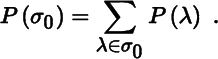
It is clear that P(σ(A)) = In. Also, if σ0 contains only one eigenvalue, say λ, then P({λ}) = P(λ). Total eigenprojections are a key concept when dealing with limits, as we shall see below.
Now consider a matrix function A(t), where A(t) is an n × n symmetric matrix for every real t. The matrix A(t) has n eigenvalues, say λ1(t), …, λn(t), some of which may be equal. Suppose that A(t) is continuous at t = 0. Then, the eigenvalues are also continuous at t = 0 (Rellich 1953).
Let λ be an eigenvalue of A = A(0) of multiplicity m. Because of the continuity of the eigenvalues, we can separate the eigenvalues in two groups, say λ1(t), …, λm(t) and λm+1(t), …, λn(t), where the m eigenvalues in the first group converge to λ, while the n − m eigenvalues in the second group also converge, but not to λ. The total eigenprojection P({λ1(t), …, λm(t)}) is then continuous at t = 0, that is, it converges to the spectral projection P(λ) of A(0) (Kato 1976).
Kato's result does not imply that eigenvectors or eigenprojections are continuous. If all eigenvalues of A(t) are distinct at t = 0, then each eigenprojection Pj(t) is continuous at t = 0 because it coincides with the total eigenprojection for the eigenvalue λj(t). But if there are multiple eigenvalues at t = 0, then it may occur that the eigenprojections do not converge as t → 0, unless we assume that the matrix A(t) is (real) analytic. (A real‐valued function is real analytic if it is infinitely differentiable and can be expanded in a power series; see Section 6.14.) In fact, if A(t) is real analytic at t = 0 then the eigenvalues and the eigenprojections are also analytic at t = 0 and therefore certainly continuous (Kato 1976).
Hence, in general, eigenvalues are continuous, but eigenvectors and eigenprojections may not be. This is well illustrated by the following example.
We complete this section with a remark on orthogonal transformations. Let B be an m × n matrix of full column rank n. Then A = B′B is positive definite and symmetric, and we can decompose
where Λ is diagonal with strictly positive elements and S is orthogonal.
Suppose that our calculations would be much simplified if A were equal to the identity matrix. We can achieve this by transforming B to a matrix C, as follows:
where T is an arbitrary orthogonal matrix. Then,
The matrix T is completely arbitrary, as long as it is orthogonal. It is tempting to choose T = In. This, however, implies that if B = B(t) is a continuous function of some variable t, then C = C(t) is not necessarily continuous, as is shown by the previous discussion. There is only one choice of T that leads to continuity of C, namely T = S, in which case
9 THE DIFFERENTIAL OF EIGENVALUES AND EIGENVECTORS: SYMMETRIC CASE
Let us now demonstrate the following theorem.
We have chosen to normalize the eigenvector u by u′u = 1, which means that u is a point on the unit ball. This is, however, not the only possibility. Another normalization,
though less common, is in some ways more appropriate. If the eigenvectors are normalized according to (41), then u is a point in the hyperplane tangent (at u0) to the unit ball. In either case we obtain u′du = 0 at X = X0, which is all that is needed in the proof.
We also note that, while X0 is symmetric, the perturbations are not assumed to be symmetric. For symmetric perturbations, application of Theorem 2.2 and the chain rule immediately yields
and
where Dn is the duplication matrix (see Chapter 3).
Exercises
- 1. If A = A′, then Ab = 0 if and only if A+b = 0.
- 2. Consider the symmetric 2 × 2 matrix
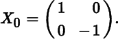
When λ0 = 1 show that, at X0,
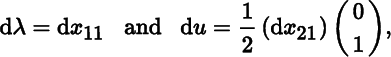
and derive the corresponding result when λ0 = −1. Interpret these results.
- 3. Now consider the matrix function
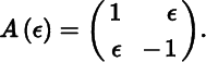
Plot a graph of the two eigenvalue functions λ1(ɛ) and λ2(ɛ), and show that the derivative at ɛ = 0 vanishes. Also obtain this result directly from the previous exercise.
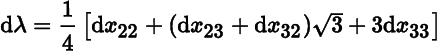
- 4. Consider the symmetric matrix
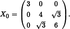
Show that the eigenvalues of X0 are 3 (twice) and 7, and prove that at X0 the differentials of the eigenvalue and eigenvector function associated with the eigenvalue 7 are
and
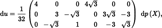
where
p(X) = (x12, x22, x32, x13, x23, x33)′.
10 TWO ALTERNATIVE EXPRESSIONS FOR dλ
As we have seen, the differential (36) of the eigenvalue function associated with a simple eigenvalue λ0 of a symmetric n × n matrix X0 can be expressed as
where u0 is the eigenvector of X0 associated with λ0:
The matrix P0 is idempotent with r(P0) = 1.
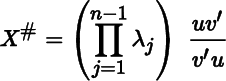
Let us now express P0 in two other ways: first as a product of n − 1 matrices and then as a weighted sum of the matrices ![]() .
.
Exercise
- 1. Show that the elements in the first column of V−1 sum to one, and the elements in any other column of V−1 sum to zero.
11 SECOND DIFFERENTIAL OF THE EIGENVALUE FUNCTION
One application of the differential of the eigenvector du is to obtain the second differential of the eigenvalue: d2λ. We consider only the case where X0 is a symmetric matrix.
Exercises
- 1. Show that Equation ( 49
) can be written as

and also as

- 2. Show that if λ0 is the largest eigenvalue of X0, then d2λ ≥ 0. Relate this to the fact that the largest eigenvalue is convex on the space of symmetric matrices. (Compare Theorem 11.5.)
- 3. Similarly, if λ0 is the smallest eigenvalue of X0, show that d2λ ≤ 0.
MISCELLANEOUS EXERCISES
- 1. Consider the function

where A is positive definite and X has full column rank. Show that

(For the second differential, see Miscellaneous Exercise 4 in Chapter 10.)
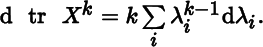
- 2. In generalizing the fundamental rule dxk = kxk−1 dx to matrices, show that it is not true, in general, that dXk = kXk−1 dX. It is true, however, that

Prove that this also holds for real k ≥ 1 when X is positive semidefinite.
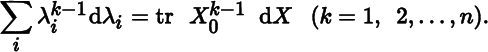
- 3. Consider a matrix X0 with distinct eigenvalues λ1, λ2, …, λn. From the fact that
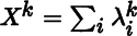 deduce that at X0,
- 4. Conclude from the foregoing that at X0,
Write this system of n equations as
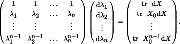
Solve dλ1. This provides an alternative proof of the second part of Theorem 8.10.
- 5. At points X where the eigenvalues λ1, λ2, …, λn of X are distinct, show that
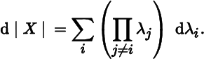
In particular, at points where one of the eigenvalues is zero,
where λn is the (simple) zero eigenvalue.
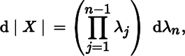
- 6. Use the previous exercise and the fact that d|X| = tr X# dX and dλn = v′(dX)u/v′u, where X# is the adjoint matrix of X and Xu = X′v = 0, to show that
at points where λn = 0 is a simple eigenvalue. (Compare Theorem 3.3.)
- 7. Let F : S → ℝm × m(m ≥ 2) be a matrix function, defined on a set S in ℝn × q and differentiable at a point X0 ∈ S. Assume that F(X) has a simple eigenvalue 0 at X0 and in a neighborhood N(X0) ⊂ S of X0. (This implies that r(F(X)) = m − 1 for every X ∈ N (X0).) Then,

where
 and
and 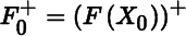 . Show that
  if F(X0) is symmetric. What is R0 if F(X0) is not symmetric?
 - 8. Let F : S → ℝm × m(m ≥ 2) be a symmetric matrix function, defined on a set S in ℝn × q and differentiable at a point X0 ∈ S. Assume that F(X) has a simple eigenvalue 0 at X0 and in a neighborhood of X0. Let F0 = F(X0). Then,
- 9. Define the matrix function
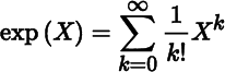
which is well‐defined for every square matrix X, real or complex. Show that
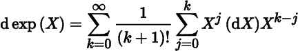
and in particular,
tr(d exp(X)) = tr(exp(X)(dX)).
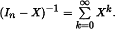
- 10. Let Sn denote the set of n × n symmetric matrices whose eigenvalues are smaller than 1 in absolute value. For X in Sn, show that
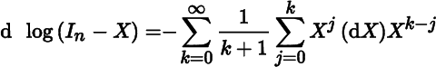
- 11. For X in Sn, define
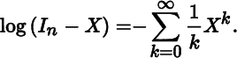
Show that
and in particular,
tr(d log(In − X)) = − tr((In − X)−1dX).
BIBLIOGRAPHICAL NOTES
3. The second proof of the Theorem 8.1 is inspired by Brinkhuis (2015).
5. Proposition 8.1 is due to Penrose (1955, p. 408) and Proposition 8.2 is due to Hearon and Evans (1968). See also Stewart (1969). Theorem 8.5 is due to Golub and Pereyra (1973).
7. The development follows Magnus (1985). Figure 8.1 was suggested to us by Roald Ramer.
8. This section is taken, slightly adjusted and with permission from Elsevier, from De Luca, Magnus, and Peracchi (2018). The relevant literature includes Rellich (1953) and Kato (1976, especially Theorems 1.10 and 5.1). The example is due to Kato (1976, Example 5.3). Theorem 8.8 is essentially the same as Horn and Johnson (1991, Theorem 6.2.37) but with a somewhat simpler proof.
9–11. There is an extensive literature on the differentiability of eigenvalues and eigenvectors; see Lancaster (1964), Sugiura (1973), Bargmann and Nel (1974), Kalaba, Spingarn, and Tesfatsion (1980, 1981a, 1981b), Magnus (1985), Andrew, Chu, and Lancaster (1993), Kollo and Neudecker (1997b), and Dunajeva (2004) for further results.