Rigging with the Joint tool is most often associated with character animation, not necessarily effects. However, joints are really just another deformer. Sure they get their own set of menus and a whole bunch of cool options, but when you get right down to it, their main purpose is to deform geometry. In this chapter we'll look at some ways to take advantage of the specialproperties joints have and use them to create some cool effects.
Chapter Contents
The Vibrating Rig: Making a Tentacle Shake
Inverse Kinematic Splines: Making a Tentacle Climb
Joints and Constraints:The Telescopic Car Suspension Rig
The Inverse Kinematic Spline Tool and Lattices
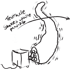
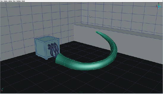
The art director shows up at your station in a panic. A shot that has already been animated is due for client review in an hour and the original animator neglected to add a shaking effect to a thrashing tentacle. The client specifically requested this in the last meeting and so it's not like it can be left out. How hard would it be to add a sort of spastic shaky effect to the scene? As usual, you say, "No problem," before even looking at the scene. When will you ever learn?
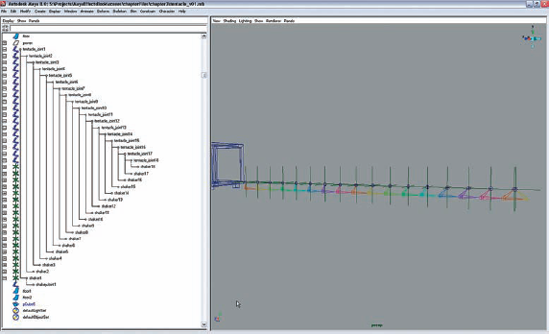
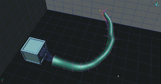
The scene shows a long alien tentacle hooked up to some kind of machine. Apparently some misguided scientists are hard at work trying to revive this severed member. Hit play on the animation and you'll see they were fairly successful at getting it to thrash about. The trick is to get this thing to shake as though electricity were being pumped into it without having to redo the animation (Figure 3.1).
First we'll take apart the original rig that the animator created so that we can implement our electrified shaky rig.
Rewind the scene to the beginning. All the joints are in the same position they were in when the tentacle geometry was skinned to the joints.
In the Outliner, select the tentacle and switch to the Animation menu set. Choose Skin >Detach Skin.
If you play the animation, you'll see that the joints still move around but the tentacle lies limp on the ground.
There are many ways to make an object shimmy and shake in Maya. In the previous chapter you saw how particles can be used to add a bumpy motion to an animated camera. In this case, a similar particle rig could be tricky; a much easier method would be the use of an animated Fractal texture applied to a joint.
Create a locator and name it "shaker1."
Open the Hypershade and create a Fractal Noise 2D texture.
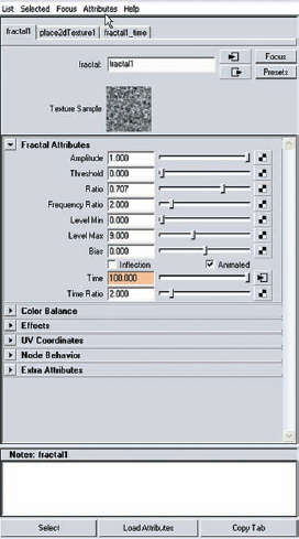
Open the Attribute Editor for the Fractal texture. Under Fractal Attributes, click the Animated check box. A number of additional attributes will become available.
Rewind the animation to the beginning. In the Attribute Editor for the Fractal texture, right-click over the numeric field for Time and choose Set Key (Figure 3.2).
Move the playhead for the animation to frame 50 or so, move the slider next to the Time attribute in the Fractal texture's Attribute Editor to about 100 or so, and set another key.
Click the arrow box to the right of the Time Slider attribute and in the fractal1_time attributes, set the Post Infinity menu to Cycle.
In the Outliner, select the shaker1 locator and MMB drag it to the work area in the Hypershade. Make sure that the new fractal1 texture is there as well.
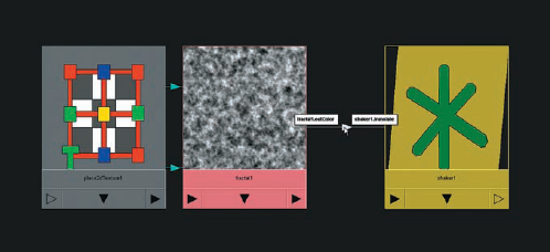
Select the fractal1 texture and MMB drag it on top of the shaker1 locator in the Hypershade. From the pop-up menu, choose Translate (Figure 3.3).
Rewind the animation. In the perspective view, zoom in on the shaker1 locator and play the animation. Wow! That thing is bugging out!
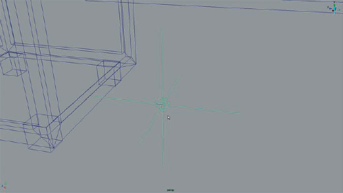
From the Animation menu set, choose the Joint tool. Click once in the perspective view to create a single joint. Rename it "shakyJoint1."
Parent shakyJoint1 to the shaker1 locator. Set the joint's Translate values to 0 in the Channel Box so the joint snaps to the same position as the locator (Figure 3.4).
We need to create a similar shakyJoint setup for each of the tentaclejoints, which means repeating the previous steps 17 more times so we have a total of 18 animated Fractal textures, 18 shaky locators, and 18 shaky joints. Luckily we can do this in one easy step.
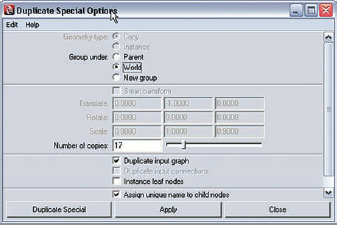
Select the shaker1 locator and use Maya 8's new duplicate special options by choosing Edit > Duplicate Special > Options. In the options, set Group Under to World and Number Of Copies to 17 and click on Duplicate Input Graph and Assign Unique Names To Child Nodes (as in Figure 3.5). Click Apply.
Seventeen new shaky locators appear. Each has its own shaky joint and its own animated Fractal texture. You can see this if you open the Hypershade and look in the Texture tab. This is all due to the fact that Duplicate Input Graph was activated.
We'll use a little bit of MEL to complete the task of parenting the shaky joints to the original, animated joints.
Our next task involves parenting each shaker joint to its respective tentacle joint (Figure 3.6). To do this we will use a little bit of MEL just to save ourselves some time and trouble. Type the following code into the Script Editor and press the Enter key on the numeric keypad to have it execute:
for ($i=l; $i<=18; $i++) {
parent ("shaker" + $i) ("tentacle_joint" + $i);
}
This bit of MEL is a simple loop that parents each of the respective shakyJoints to its respective tentaclejoint. The loop first initializes the variable $i by setting it to 1. The $i++ increments $i by 1 each time it runs, as long as $i is less than or equal to 18. In the body of the loop we append $i to the name of the parent joints and the tentaclejoints so Maya knows which objects to parent to which. It's three lines of code that saves us a whole lot of clicking.
Note
Notice that each shaker pops into place when you parent it. This is because the translate values already have an input connection (the Fractal texture) that is pretty close to 0,0,0 for XYZ. Remember that when you parent an object to another object and then "zero out" its translate values, the child object pops right to the pivot point of its parent. It's as if the parent is now the origin for the child. The Fractal texture, with values being close to 0,0,0, is doing this zeroing out of the translate values for us. Very handy.
Play the animation. The shaking locators now follow the animation of their parent joints. All of them shake exactly the same way though, which is not what we want.
The easiest way to mix up the vibration of the joints is to rotate the place2D texture node attached to each Fractal texture. We could open the attribute for each node and randomly move the slider, or we could put MEL to work for us again and take away some of the tedium. Type the following code into the Script Editor and press the Enter key on the numeric keypad to have it execute:
for ($i=l; $i<=18; $i++){
 setAttr ("place2dTexture" + $i + ".rotateUV") (rand(360));
}
This is similar to the last bit of code we used in that it is a simple loop that runs as long as $i is less than or equal to 18. In the body of the loop, Maya has to set the rotateUV attribute for each place2dTexture node to a random number from 0 to 360. When you use the rand function with a single number in parentheses, Maya assumes you mean a number from 0 to the specified value; it's the same as writing rand(0,360).
You'll see that when the animation plays, each shaker moves about in a different way.
Next, we need to reconnect the tentacle to our shaky joints.
We will be skinning the tentacle to the new shaky joints, but before we do this, we have to get them as close as possible to the starting position of the tentaclejoints. If you rewind the animation, you'll notice that they are slightly offset from the position of each tentacle joint. This is because the animated fractal is now feeding the translate values for each shaky locator a random value from 0 to 1.
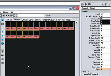
Open the Hypershade and switch to the Texture tab. Shift+select all the textures. In the Channel Box, find the Color Gain R, G, and B values. Set them all to 0. The shake locators should pop to the position of the tentacle joints. The fractal textures will turn black when you do this (Figure 3.7).
In the Outliner, Ctrl+select each shaky joint. Then Ctrl+select the tentacle. Alternatively, you can save some time by using the MEL select command. Type this into the command line:
select -r "shakyJoint*";
The r flag stands for replace, as in "replace the current section." The asterisk after shakeyjoint is a wildcard that tells Maya to select all the objects whose names start with "shakyJoint." Since our shaky joints are numbered 1 through 18, Maya knows to select all of them. Once they're selected, Ctrl+select the tentacle.
From the Animation menu set, choose Skin > Bind > Skin > Smooth Bind > Options. In the options, set Bind To to Selected Joints, Bind Method to Closest Distance, Max Influences to 3, and Dropoff Rate to 4.
The animation now looks just like it did when we started, but that's good. The only reason it's not shaking is because we turned off the shakiness of the Fractal textures by setting the Color Gain values to 0.
At this point we could turn up the Color Gain values on each Fractal texture to get the vibration back; we could even set different values so that the end of the tentacle shakes more than at the base. For now let's create a slider control that takes care of all of the shakers at once. Think of it as a dimmer switch for the shakes.
Create a new locator and name it "shakeControl."
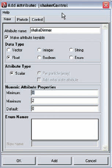
Open the Attribute Editor for shakeControl and choose Attributes > Add Attribute.
Name the attribute "shakeDimmer." Set Data Type to Float, and enter 0 for Minimum, 2 for Maximum, and 0 for Default (Figure 3.8).
Note
You may notice that when we create a custom attribute and name it using the convention "customAttribute," Maya will automatically label the attribute as two separate, capitalized words. However, when we refer to this attribute in an expression, we still need to type it in the Expression Editor using our original "customAt-tribute" syntax.
Open the Connection Editor and load the shakeControl locator on the left side.
Open the Hypershade and select fractal3 (we'll leave fractal1 and fractal2 alone for now).
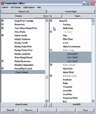
In the Connection Editor, connect the Shake Dimmer attribute on the left side to the Color Gain R, G, and B values on the right. Do this for fractal3 through fractal18 (Figure 3.9).
Since fractal1 and fractal2 control the shakers nearest the thick end of the tentacle where the generator model is hooked up, we can leave their Color Gain values at 0 or near 0 just so the shaking doesn't get out of hand.
Set the Shake Dimmer attribute to 0.5 and play the animation. If all goes as planned, you should see the original animation with a bit of quaking added to the movement of the tentacle (Figure 3.10). You can keyframe the Shake Dimmer attribute so that the shaking gets worse over time. Setting it at a value between 1 and 2 will create some really crazy shakes.
This next shot occurs later in the severed tentaclefilm. At this point, the alien is upset and still holding a grudge against those who have removed its tentacle. In this shot, we see a close-up of a pipe; a tentacle wraps around the pipe as the alien makes its way through the plumbing somewhere beneath the lab.
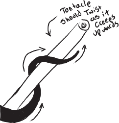
Wrapping a tentacle around a piece of geometry is a pretty straightforward operation. However, we want to add the effect of the tentacle creeping up toward the camera as it wraps around the pipe. To do this, we'll use a combination of regular forward kinematics and the Inverse Kinematic Spline tool.

We have a simple pipe model and the slimy tentacle. A camera has been set up for the shot. For now, hide the tentacle.
First we'll be creating a curve that wraps around the pipe. Later on we will slide the tentacle along this curve using the IK Spline tool. However, if we draw the curve directly on the pipe, we will encounter a problem when the tentacle slides along it; namely, the thickness of the tentacle will cause it to penetrate the geometry of the pipe. To work around this, we'll create an invisible cylinder for our curve that is slightly thicker than the pipe.
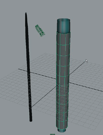
Create a NURBS cylinder that fits around the pipe up to the bulge at the top of the pipe. Name the cylinder "dummy" and give it 10 spans (Figure 3.11).
Select the dummy surface and choose Modify > Make Live. Now we can draw a curve on the surface.
Choose Create > CV Curve Tool. In the options, make sure that Curve Degrees is set to Cubic.
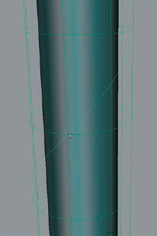
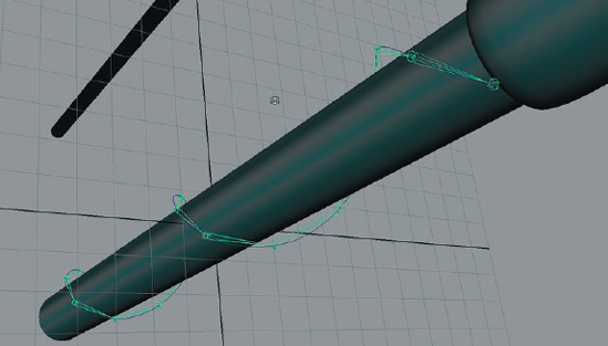
Turn grid snapping on. Starting from the top of the cylinder, click on the livedummy surface to draw a curve that wraps around the cylinder. With grid snapping on, each time you click on the surface, the new CV should snap to theisoparms of the live surface. Try to draw the curve so that each CV is one spandown and two over (see Figure 3.12).
When you've reached the bottom, hit Enter to complete the curve.
We'll add some joints to deform the curve itself; this curve will later become a path for the tentacle to follow.
We need to duplicate the curve drawn on the surface. Select Surface Curve and (from the Surfaces menu set) choose Edit Curves > Duplicate Surface Curves.
Rename the duplicated curve "tentacleCurve."
In the Outliner, select the dummy surface and hit the down arrow key to make it "unlive." Hide the dummy surface so you don't confuse the tentacle curve with the surface curve. We want to keep the dummy around so we can preserve the history connection between it and the tentacleCurve.
Select the tentacleCurve and choose Edit Curves > Rebuild Curves > Options. In the options, set Rebuild Type to Uniform and Parameter Range to "0 to 1", keep the ends, and set Number Of Spans to 12. Make sure it's a cubic curve and don't keep the original.
Turn on curve snapping, and from the bottom of the curve, start adding joints that follow along to the top. Make a chain of about 18 joints or so. When you've finished making the joints, you should rename them. Select the root joint in the Outliner. Choose Modify > Prefix Hierarchy Names. In the pop-up window, type curve_ and hit Enter. The joints will be renamed "curvejoint1," "curve_joint2," "curve_joint3," and so on.
Select curvejoint1 and (from the Animation menu set) choose Skeleton > Orient Joints > Options. In the options, choose Edit > Reset to switch to the default settings; these should work fine (Figure 3.13).
Select curve joint1 and the tentacleCurve and choose Skin > Bind Skin > Smooth Bind > Options. In the options, make sure that Bind To is set to Joint Hierarchy, Bind Method is set to Closest In Hierarchy, and Max Influences is set to 3. Go ahead and hit Apply to bind the curve to the curvejoints.
Next we'll use the joints to animate the curve coiling around the pipe.
Set the range of the animation to 60 frames. Set the playhead to frame 60.
In the Outliner, Shift+select all of the curvejoints and set a keyframe on their X, Y, and Z rotational values.
Note
An easy way to select multiple objects is to use the Sel field located on the right-hand side of the Status line. Just type tentacle joint* in this field and hit Enter. Using the asterisk wildcard will tell Maya to select all of the objects that start with tentacle joint. This can save some clicking.
Move back to frame 1. Shift+select joints 2 through 17.
Choose the Rotation tool and click on the green circle to rotate the Y axis. Slowly drag to the left so that the chain of joints unwinds (Figure 3.14).
Set a keyframe on the rotational values of these joints.
Play through the animation. The curvejoints should wrap around the dummy surface over the 60 frames.
The motion looks pretty good but it's not quite organic enough. To fix it, we'll offset some of the joints' keyframes in time.
In the Outliner, Shift+select joints 3 through 17.
Open the Graph Editor. Marquee drag around the keyframes at the start of the animation then switch to the Move tool. Hold the Shift key down and MMB drag the keys a few frames to the right.
Control+click joint 3 in the Outliner so that it is deselected; joints 4 through 16 should still be selected. Repeat the steps1 and 2 to move their keyframes to the right.
Repeat this process of moving keys and deselecting the parent joint one at a time until you've gone through all the joints up to 17.
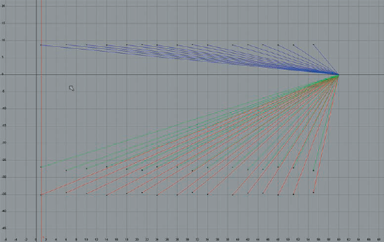
Reselect all the joints and compare what you see in the Graph Editor with Figure 3.15. It doesn't have to be exactly the same, just similar.
The animation looks a bit more natural now.
Now that we have our curve looking good, let's put some joints on the tentacle and get it ready for the IK Spline tool.
Switch to the side view.
Turn the shading display to wireframe so it's easier to see what's going on. You may want to turn the resolution of the tentacle down to rough as well (select the object and hit 1 on the keypad).
Turn grid snapping on, and starting from the top of the tentacle, add joints every two units all the way down the tentacle. Hit Enter when all of the joints have been created (Figure 3.16). Use the Prefix Hierarchy command to rename these joints "tentaclejoints."
Smooth bind the tentacle to the tentaclejoints using the settings from the section "Adding Joints to the Curve" earlier in this tutorial.
The Inverse Kinematic Spline tool allows you to control the rotations of joint in a chain using the CVs on a curve. You can either have Maya automatically create the curve or use an exisiting curve. In this case we'll use the curve we animated coiling around the pipe.
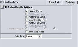
From the Animation menu set, choose Skeleton > IK Spline Handle Tool > Options. In the options, turn off Snap Curve To Root and Auto Create Curve (Figure 3.17).
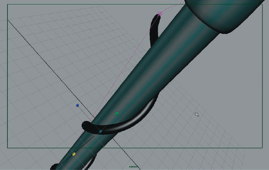
With the tool active, in the perspective view click on the tentaclejoint at the top of the tentacle, then click on the tentaclejoint at the bottom of the tentacle, and finally, carefully click on the tentacleCurve. The tentacle and its joints should jump over to the tentacle curve.
In the Outliner, select the curvejoints and turn off their Visibility (Ctrl+h) so that things are a bit easier to see.
The animation now shows the tentacle wrapping around the pipe. There are a few things we have to fix, though, before we are done.
Move to the end of the animation and switch to shaded view.
The tentacle is still offset from the pipe. In the Outliner, select the invisible dummy surface. Scale it down in X and Z until the tentacle looks like it's wrapped around the pipe properly. The history connection between the dummy surface and the tentacleCurve allows us to do this.
Switch to the camera view. From the Outliner, select ikHandle1. In the Channel Box, find the Offset attribute. It should be at 0. Set a keyframe for this value.
Move to frame 1 and set Offset to .8. Set another keyframe.
Playing through the animation from the camera view, you can see that the tentacle now moves up the pipe as it wraps around. I think this motion could be a little more obvious.
Move to frame 40 and set Offset to 0.5. Set a keyframe here. Now it's looking creepier!
You can open the Graph Editor for ikHandle1 and refine the movement of the tentacle's creep (Figure 3.18).
The next shot is for a kids cartoon. It involves a car created by a master inventor. Talk about smooth rides. As this car cruises along a series of rolling hills, the chassis of the car stays level while the wheels stayed glued to the road, all thanks to the super robotic extension suspension invented by our cartoon animator.
To accomplish this task, we need to first create a rig for our robotic extension legs that spans the gap between the car and its wheels. The animator wants to be able to move the car down the roadway and have the legs automatically extend, allowing the wheels to constantly touch the road. We can create a rig composed of joints and constraints to take care of the legs. Once that's done, we'll set up a system where the wheels stick to the road. Then we can connect the legs and the wheels. It's all very simple actually.
Most of the time when joints are used, the animation of the object they deform is based on their rotation. To create our telescopic rig we'll devise a system in which the animation of the legs is based on the scaling of the joints. And it should be noted that the use of the word "telescopic" refers to how the sections of the leg rectract in on themselves similar to how the pieces of a telescope retract in on themselves. In this case it has nothing to do with optics.
First we'll need to create the geometry for the legs.
Open up the file
extendo-LegCar_v01.mbfrom the chapter3folder on the CD.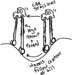
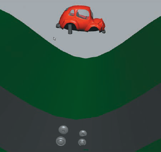
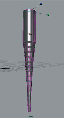
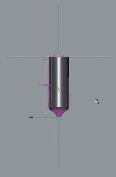
The car is hovering above the hilly roadway; its wheels are down on the ground. This is the maximum height the car will achieve. You have been instructed to create a telescopic leg that extends from the car down to the wheels. This leg will expand and contract, keeping the car level as it drives over the hills (Figure 3.19).
There is a single piece of geometry named legSection1_1 in the car's left rear wheel well. This will become our telescopic leg.
Turn off visibility for all of the display layers except the LEG and WHEELS layers.
Switch to the side view and zoom out so you can see the wheels and the leg section.
There are about 15 units between the leg section and the wheel. The leg section is one unit tall, so we'll duplicate it 15 times using the new Duplicate Special options.
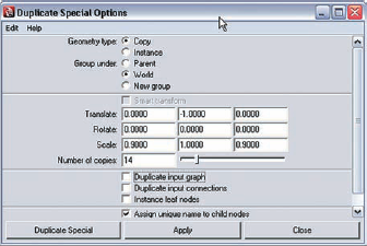
Select the legSection1_1 object and choose Edit > Duplicate Special > Options.
In the options, set Geometry Type to Copy and Group Under to World. Set Translate Y to −1 and Scale to 0.9, 1, 0.9. Set Number Of Copies to 14. Hit Apply to make the copies (Figure 3.20).
Select all the leg sections and choose Modify > Freeze Transformations.
With our first leg created, we can set up our scale-based telescopic rig to control its extension.
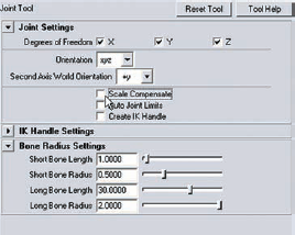
From the Animation menu set, choose Skeleton > Joint Tool > Options. In the options, turn off Scale Compensate (Figure 3.21). With Scale Compensate off, all child joints will scale to the same size as their parent joint.
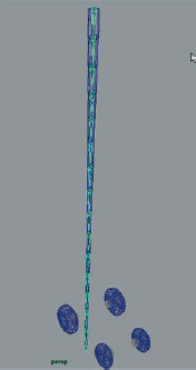
Turn on grid snapping and create a joint chain down the length of the leg. Make one joint for each leg section. Place the last joint at the bottom of the final section.
Switch to the front view. Select joint1 and move it so that the joint chain is at the center of the leg geometry (Figure 3.22).
In the Outliner, select joint2 through joint16. In the Channel Box, Shift+select the Rotate X, Y, and Z attributes. Right-click and choose Lock Selected.
Select joint1 and choose Modify > Prefix Hierarchy Names. In the field, type leg-Section1_.
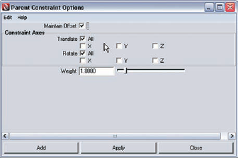
This next part is a bit tedious, but that comes with the territory sometimes. Select legSection1joint1 and Ctrl+select the legSection1_1 geometry. Choose Constrain > Parent > Options. In the options, make sure Maintain Offset is checked and that All is selected for both Rotate and Translate (Figure 3.23). The Weight setting should be at 1. A parent constraint constrains both the translate and the rotate values. As with a regular parent connection, you can still move the child node. For our purposes, don't move the child nodes. We're using this type of constraint to save time, so we don't need to create both a point and a rotate constraint for each object.
In the Outliner, go down the line and create a parent constraint so that each leg-Section is constrained to its respective legSection joint. Constrain legSection1_2to legSection1_joint2, legSection1_3 to legSection1_joint3, and so on. legSection1joint16 will not need anything constrained to it. Alternatively, you coulduse a little MEL scripting to automate this process. A simple loop like the onesused in the shaky tentacle tutorial might do the trick. Type the following into theScript Editor:
for ($i=l; $i<=16; $i++) {
  parentConstraint -mo ("legSectionl_joint" + $i) ("legSectionl_" + $i);
}
The mo flag in the parentConstraint command stands for "maintain offset." If it's not specified in the command, Maya automatically constrains all axes and gives the constraint weight of 1.
When you are done, try rotating legSection1joint1 to make sure all the geometry has been constrained to the joints. If all the leg sections rotate with the jointsproperly, good work. You may now ask yourself why we didn't just skin thegeometry to the joints. Well, I'm glad you asked.
Return legSection1joint1 to its 0, 0, 0 rotational position and try scaling down in X. You'll see all the section geometry retract just like a telescopic leg should (Figure 3.24). By using constraints instead of binding, we avoid having the geometry scale with the joint. Since we turned off Scale Compensate for the joints, all the child joints scale with the legSection1joint1 joint, which means this is the only joint we have to worry about animating.
If we scale past 1 in X for the root joint, the sections start to come apart. Let's set some limits to prevent this.
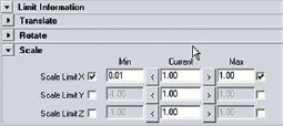
Select legSection1joint1 and open its Attribute Editor.
In the Limit Information section, expand the attributes for Scale.
Click the check box next to Scale Limit X and put .01 in the Min box and 1 in the Max box (Figure 3.25).
Next, we'll create an Inverse Kinematic handle so that the leg always points toward the end of the joint chain.
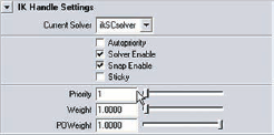
Switch to wireframe mode in the perspective view, and from the Animation menu set, choose Skeleton > IK Handle Tool > Options. In the options, switch Current Solver to ikSCsolver. Turn off Sticky (Figure 3.26). The SC solver is a single chain solver. Since we are not concerned about the rotation of the child joints, a single chain solver will do fine (as opposed to the RP, or rotate plane, solver, which adds twist controls to adjust the rotation of the child joints).
With the IK Handle tool active, click on legSection1joint1 at the top of the joint chain and then click on legSection1_joint16.
Create a locator and name it "legWheel_1."
Turn on point snapping and place the legWheel_1 locator at the same location as the newly created IK handle at the bottom of the joint chain.
With legWheel_1 selected, choose Modify > Freeze Transformations to zero out its Rotate and Translate attributes.
Select legWheel_1 and ikHandle1 in the Outliner. Choose Constrain > Point to lock the IK handle to legWheel_1. Select ikHandle1 and turn off its Visibility (Ctrl+h) so you don't accidentally select it in the future.
Finally, we'll create a control that will automatically scale the leg based on its distance from the wheel.
Switch to the side view and choose Create > Measure Tools > Distance Tool.
With point snapping on, click on the joint at the top of the chain.
Zoom in closely to the legWheel_1 locator on the bottom of the joint chain, and click on it carefully to connect the Distance tool to this locator. You should see two arrows appear between a new locator at the top of the chain and the legWheel_1 locator. The number 15 should appear between the arrows (Figure 3.27).
Rename Locator1 "legTop_1" and point constrain the legSection1joint1 joint to legTop_1.
Select the legSection1joint1 joint and scale it down to .01 in X so that the entire leg retracts.
Select the legWheel_1 locator and translate it in Y so that it is right at the tip of the bottom of the retracted leg (Figure 3.28).
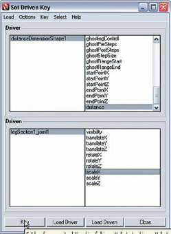
In the Animation menu set, choose Animate > Set Driven Key > Set. The Set Driven Key window will open.
In the Outliner, set the display mode so that shape nodes are available, and then scroll down and choose the distanceDimension1's shape node. Load it as the Driver in the Set Driven Key window.
Select the legSection1joint1 joint and load it as the Driven in the Set Driven Key window.
On the right section of the top part of the Set Driven Key window, scroll down and choose the Distance attribute.
In the bottom right, choose the ScaleX attribute.
Hit the Key button (Figure 3.29).
Select the legWheel_1 locator, and in the channel box, set the TranslateX, Y, and Z values to 0.
Select the legSection1joint1 joint and set the ScaleX value to 1.
Click the Key button in the Set Driven Key window.
When you move the legWheel_1 locator up and down, the leg should automatically retract.
Duplicating this rig is easy, by using Duplicate Special, we can avoid having to repeat the process of building the rig from scratch.
Select all of the leg geometry and group it. Rename the group "leg_1."
Select the leg_1 group and choose Edit > Duplicate Special > Options. Set Group Under to World and Number Of Copies to 1, and check Duplicate Input Graph and Assign Unique Name To Child Nodes.
These Duplicate Special settings will duplicate all of the geometry, the joints, the locators, and the distance dimension. including the set driven keys that automate the scaling. The only thing that will not duplicate is the ikHandle.
Hide all the leg1 objects, joints, locators, and so on.
Expand the new set of joints associated with leg 2.
At the bottom of the joint chain in the Outliner, delete the effector.
Create a new IK handle using the steps described in the section "Creating an IK Handle for the Leg Joints" earlier in this tutorial. Hide it and point constrain it to legWheel_2.
Make two more duplicate legs using this process. If the newly duplicated legs appear all blue, apply a new shader to them. Sometimes the shading does not duplicate very well. Remember to rename all the joints and geometry associated with leg 2 so that instead of legSection1 they read legSection2. You can use Search and Replace Names under the Modify menu to do this.
The next few steps involve positioning the duplicated legs in relation to the car.
When you have four legs, turn the visibility for the CAR layer back on.
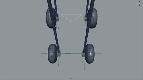
Place the leg top locators in each of the wheel wells of the car so that legTop_1 is in the driver side front wheel well, legTop_2 is in the driver side rear wheel well, legTop_3 is in the passenger side rear wheel well, and legTop_4 is in the passenger side front wheel well (Figure 3.30).
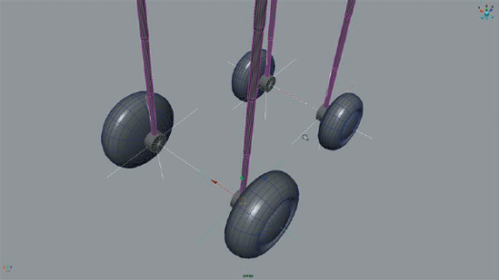
Arrange the legWheel locators so that they are at the center point of the cylinder attached to the inside of each wheel (Figure 3.31).
When you have these arranged, select each of the legTop locators and choose Modify > Freeze Transformations to zero out their translate values. Do the same for the legWheel locators.
You may want to hide the distance dimension objects just to make the scene a bit clearer.
We'll use parent constraints to attach the wheels to the legs.
Select legWheel_1 and then Shift+select the L_front_tire object.
Create a parent constraint between the two objects.
Do the same for the other three wheels, parent constraining the wheels to the legWheel locators.
We can create some controls using NURBS curves to make the task of animating the car a bit easier.
Switch to the top view and turn on grid snapping.
Choose Create > CV Curve Tool > Options. Set Curve Tool Degree to Linear.
In the top view window, draw a triangle on the grid using four points.
Choose Modify > Center Pivot to set the pivot at the center of the triangle.
Rename the triangle frontSuspension.
Duplicate the triangle and name the duplicate rearSuspension.
Scale the triangles down a little bit and move them so that the frontSuspension object is in between the front wheels and the rearSuspension object is in between the rear wheels (Figure 3.32).
Freeze their transformations once you are happy with their placement.
Parent legWheel1 and legWheel4 under the frontSuspension triangle.
Parent legWheel2 and legWheel3 under the rearSuspension triangle.
Note
We could have used locators for the suspension objects, but after a while it starts to look like a mess. The triangles are slightly more visually appealing.
Move the front suspension object around, rotating it on its Y axis. You now have a nice control for the car's steering, yet the wheels can also move independently since they are parented under the front suspension control. To return them to their original positions, you can just zero out their transforms.
Note
We can connect the car to a motion path to automate its movement across the terrain, then all we have to keyframe are the wheels and the chassis.
Select all the leg controls in the Outliner and add them to the LEGS display layer by right-clicking over the LEGS layer in the Layer Editor and choosing Add Selected Objects.
Turn off the visibility for the CAR, LEGS, and WHEELS layers. Turn on the visibility for the GROUND layer.
Select the road object in the perspective view, right-click, and choose Isoparms.
Select the isoparm at the center of the road. Switch to the Surfaces menu set and choose Edit Curves > Duplicate Surface Curves. Rename the new curve "carPath."
Create a locator and name it "wheelFollow."
Switch to the Animation menu set and choose Animate > Motion Paths > Attach To Motion Path > Options.
In the options, choose Edit > Reset Options. These should work just fine. We want Follow on so the locator rotates to follow the contour of the motion path.
Turn the visibility of the other layers back on, and move the playhead so that the wheel follow locator is below the car—around frame 88 or 89.
Parent the frontSuspension and rearSuspension objects to the wheelFollow locator.
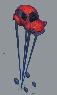
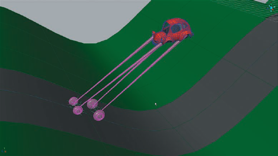
Scrub back and forth on the Time Slider. You should see the wheels climb up and down the hilly road. The legs should point toward the wheels (Figure 3.33).
Set the playhead back to frame 88. Create a new locator and name it "chassis-Control."
Place the chassis control at the center of the chassis object. The easiest way to do this is to point constrain the locator to the chassis object (make sure Maintain Offset is Off in the Point Constraint options). The locator should snap to the center of the chassis. Then, in the Outliner, delete the point constraint from under the chassisControl object. Freeze transforms on the chassisControl.
Parent each of the legTop locators to the chassis control locator.
Almost there! Create yet another locator and name it "carFollow." Place it at the same location as the chassis control locator.
Point constrain carFollow to the wheelFollow object. In the options for the point constraint, turn Maintain Offset on and set Constraint Axes to Z Only.
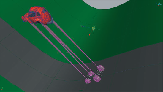
As you scrub back and forth in the Timeline, the carFollow locator should move with the wheelFollow but maintain a level height (Figure 3.34).
Move the Time Slider back to frame 88 and parent chassisControl to the carFollow locator.
Parent constrain the Chassis object to the chassisControl locator.
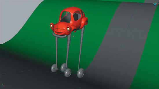
As you move back and forth on the Time Slider, the car should remain level while the telescoping suspension legs follow the road. That's one smooth ride!
If the car is moving backwards, you can select the wheelFollow locator, open its Graph Editor for the motion path node, and reverse the keyframes so that it's moving in the correct direction.
The animator has the advantage of an automated system to control the extension of the legs, but he can also independently keyframe the front and rear suspension and each of the wheels as well as the chassis. This way he can make the legs a little more wobbly as well as move the chassis around as if it's having a hard time balancing on top of the wobbly legs. Hey, this is a prototype car; it's bound to have a few kinks in it. He will certainly have to make adjustments as the car reaches the crest of each hill. A few keyframes on the chassisControl object should fix these problems.
The telescoping rig created for the legs holds a lot of promise for experimentation. See how you can augment the current rig or repurpose it for other models.
Try applying an animated Fractal texture to the movement of the chassis to get a nice shakiness to the car as it putters along.
Create a system where the front and rear suspension have their own motion paths to follow. See if you can improve on the controls so that the animator can easily see and select the chassis and wheel controls.
See if you can create some custom control objects, like the triangle used for the front and rear suspension, so that the animator can easily access controls for the chassis and each wheel without worrying about clicking or moving the wrong thing.
What if, heaven forbid, the art director suddenly decides that the legs need to bend a little to add some squash and stretch? See if you can either design a rig with this built in or alter your current rig. Chapter 4 might hold some clues. A clever use of a blend shape and wire deformers applied to the leg geometry groups might allow you to achieve this.
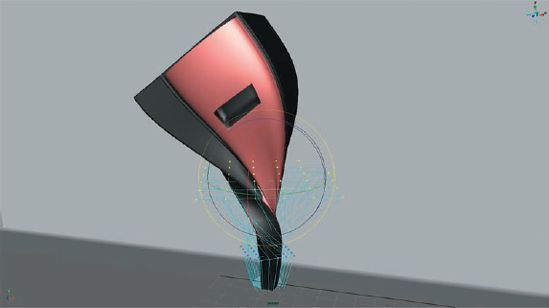
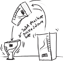
A commercial shot requires you to make a soda machine disappear into a black hole in the ground. The client would like the machine to fly up into the air, follow an arc, and then get sucked into the hole top first. The machine should shrink as it goes through the black hole.
Instead of skinning the geometry of the soda machine to a joint chain, we'll skin a lattice that deforms the soda machine. This allows for a smooth deformation that's easy to set up. Our first task is creating the lattice.
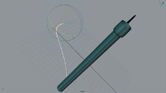
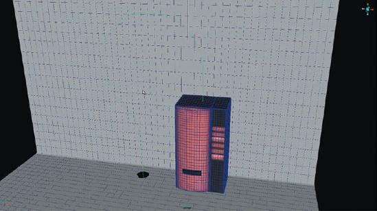
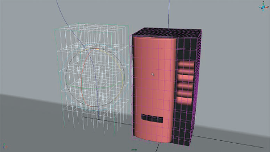
The machine has been built as a single polygon object. The modeler has also provided a curve for the machine to follow as it makes its way through the hole (Figure 3.36).
If you play the animation, you'll see a little hole open up when the curve meets the floor at about frame 20. This hole was created by projecting a circle on the floor, trimming the surface, and then setting keyframes on the scale of the projecting curve.
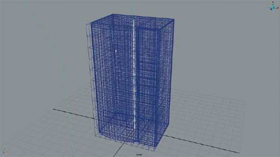
First let's create a lattice around the machine. Switch to the Animation menu set and choose Deform > Create Lattice.
In the Channel Box for the lattice shape, set the S, T, and U Divisions to 12.
In the Attribute Editor for the ffd1 node, uncheck the Local box. This makes the deformation smoother but a little less accurate.
The next task is creating joints for the lattice.
Switch to the front view and turn on wireframe shading.
Zoom into the soda machine and turn on grid snapping.
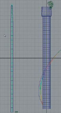
Select the Joint tool and reset the settings in the Tools option window. Starting at the bottom of the soda machine, create a joint chain going straight up the center. Make each joint one unit tall so that the resulting chain is 14 joints long.
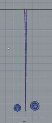
Because of the positioning of the models, the joint chain will be at the same position as the curve (Figure 3.37). Isn't that handy?
Select the joint chain and the ffd1Lattice object in the Outliner (don't select the ffdbase). Choose Skin > Smooth Bind to bind the lattice to the joints. In the options, you can use the Edit menu to reset the options to the default settings, which should work fine.
An IK Spline can be created for the joints using the motion path curve that already exists in the scene.
Choose Skeleton > IK Spline Handle Tool > Options. In the options, click Root On Curve and Auto Parent Curve. Turn off Snap Curve To Root and Auto Create Curve.
With the IK Spline Handle tool active, move to the perspective window and click on the joint at the bottom of the machine, then the joint at the top, and then the path curve.
Open the Channel Box for the ikHandle1 tool and find the Offset attribute toward the bottom of the Channel Box. Leave the value at 0 and set a keyframe at frame 1.
Move the playhead to frame 30 and set the offset to 1. Set another keyframe.
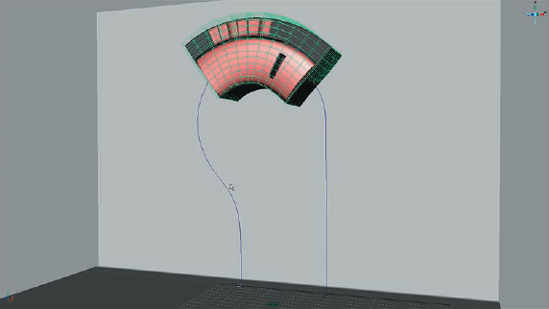
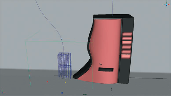
When you play the animation, you'll see the soda machine leap into the air and then go through the hole in the ground (Figure 3.38).
To create the squashing effect, we'll put a second lattice on top of the first lattice that is deforming the machine.
In the Outliner, select the ffd1Lattice object.
Choose Deform > Create Lattice to make a new lattice.
In the Channel Box for the new lattice, set the S, T, and U Divisions to 6.
In the Outliner, select both the ffd2Lattice object and the ffd2Base object. Move them over to the left so that they are over the hole in the floor. The machine should not deform when you do this. If it does, make sure you have both the lattice and the base selected. Rotate the second lattice and its base object 180 degrees in Z (Figure 3.39).
Move the playhead to frame 19.
Adjust the second lattice and base so that they are at the same position as the machine. Move them down a little so that they're halfway through the floor.
You may want to hide the first lattice and base just so you don't get confused about what you're looking at.
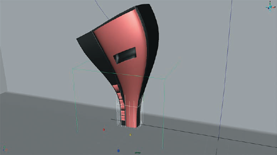
Select the second lattice and scale it down in X and Z. Scale the lattice base up a little so that the machine looks like it does in Figure 3.40.
Have some fun creating a nice squash effect by adjusting the scale on the second lattice and the size of its base. Right-click over the lattice and choose Lattice Points. Select the lattice points and scale them down. It will take some tweaking to get just what you want. Move the animation back and forth and continue to fool around until it looks good.
Move to the start of the animation. If you notice that the machine is deformed in a weird way (as in Figure 3.41), it may be that the base for lattice2 has been scaled up too high. Scale it down again until this goes away.
There are a couple of ways we can add a twist to the soda machine to make its movement a little more interesting.
Right-click over the second lattice and choose to select the lattice points.
Select the lower rows of lattice points and use the Rotate tool to rotate them in Y about 45 degrees. This should create a nice twisting effect as the machine gets sucked into the hole.
You can also set keyframes on the ikHandle's Twist and Roll attributes to enhance this twisting effect. This may require further tweaking of the lattice to work correctly. The twist control is a lot of fun to play with; experiment with it to get some interesting effects. For this particular shot, however, rotating the lattice points on the second lattice may work better (Figure 3.42).