
4
Microgrid Protection
4.1 Introduction
One of the major technical challenges associated with a wide deployment of microgrids is the design of its protection system. Protection must respond both to the utility grid system and to microgrid faults. If the fault is on the utility grid, the desired response is to isolate the microgrid from the main utility as rapidly as necessary to protect the microgrid loads. The speed of isolation is dependent on the specific customer's loads on the microgrid, but it probably requires the development and installation of suitable electronic static switches. Electrically operated circuit breakers in combination with directional over-current protection is another possible option. If the fault is within the microgrid, the protection system isolates the smallest possible section of the distribution feeder to eliminate the fault [1]. A further segmentation of the microgrid during the isolated operation, that is, a creation of multiple islands or sub-microgrids, must be supported by microsource and load controllers.
Most conventional distribution protection is based on short-circuit current sensing. The presence of DERs might change the magnitude and direction of fault currents, and might lead to protection failures. Directly coupled rotating-machine-based microsources will increase short-circuit currents, while power electronic interfaced microsources can not normally provide any significant levels of short-circuit currents required. Some conventional over-current sensing devices will not even respond to this low level of over-current, and those that do respond will take many seconds to do so, rather than the fraction of a second that is required. Thus, in many operating conditions of microgrids, problems related to selectivity (false, unnecessary tripping), sensitivity (undetected faults) and speed (delayed tripping) of protection system may arise.
Issues related to protection of microgrids have been addressed in several publications [2–5]. The major problems can be summarized as:
- changes in the value and direction of short-circuit currents, depending on whether a distributed generator is connected or not,
- reduction of fault detection sensitivity and speed in tapped DER connections,
- unnecessary tripping of utility breaker for faults in adjacent lines, due to fault contribution of DER,
- increased fault levels may exceed the capacity of the existing switchgear,
- auto-reclosing and fuse-saving of the utility line breaker policies may fail,
- reduced fault contribution of inverter based DER on protection system performance, especially when isolated from the utility grid,
- conflict between the feeder protection and utility requirements for fault ride through (FRT) which is included in the grid codes of many countries with a large penetration of DER,
- effect of closed-loop and meshed distribution network topologies with DER.
This chapter presents a protection solution for microgrids that can overcome some of the above problems. This is based on automatic adaptive protection, that is, change of protection settings depending on the microgrid configuration based on pre-calculated or on real-time calculated settings. The increase in the fault current level helped by a dedicated device, especially in isolated operation of microgrids dominated by power electronics interfaced DER, is also analyzed. Finally, the possible use of fault current limitation is discussed.
4.2 Challenges for Microgrid Protection
4.2.1 Distribution System Protection
Generally a distribution system (including a microgrid) is divided into local protective zones which are covered either by a network (overhead lines and cables) or apparatus (buses, transformers, generators, loads etc.) protection (Figure 4.1).
Figure 4.1 Protection zones of different MV and LV circuit breakers with over-current relays for grid elements and apparatuses
Requirements which provide a basis for design criteria of a distribution protection system are known as “3S” which stands for:
- sensitivity – protection system should be able to identify an abnormal condition that exceeds a nominal threshold value.
- selectivity – protection system should disconnect only the faulted part (or the smallest possible part containing the fault) of the system in order to minimize fault consequences.
- speed – protective relays should respond to abnormal conditions in the least possible time in order to avoid damage to equipment and maintain stability.
“3S” can be extended by:
- dependability – protection system must operate correctly when required to operate (detect and disconnect all faults within the protected zone) and shall be designed to perform its intended function while itself experiencing a credible failure.
- security – protection system must not operate when not required to operate (reject all power system events and transients that are not faults) and shall be designed to avoid misoperation while itself experiencing a credible failure.
- redundancy – protection system has to care for redundant function of relays in order to improve reliability. Redundant functionalities are planned and referred to as backup protection. Moreover, redundancy is reached by combining different protection principles, for example distance and differential protection for transmission lines.
- cost – maximum protection at the lowest cost possible.
4.2.1.1 Over-Current and Directional Over-Current Protection
The protection of distribution grid, where feeders are radial with loads tapped-off along feeder sections, is usually designed assuming a unidirectional power flow. It is based on a detection of high fault currents using fuses, thermo-magnetic switches and molded case circuit breakers with standard over-current (OC) relays (ANSI 51) with time-current discriminating capabilities. More sophisticated directional OC relays (ANSI 67) are used for the protection of ring and meshed grids.
4.2.1.2 Distance Protection
Some utilities install distance relays (ANSI 21) for line protection. The distance relay compares the fault current against the voltage at the relay location to calculate the impedance from the relay to the faulted point. As a rule of thumb, a distance relay has three protection zones: zone 1 covers 80–85% length of the protected line, zone 2 covers 100% length of the protected line plus 50% of the next line, zone 3 covers 100% length of the protected line plus 100% of the second line, plus 25% of the third line. If a fault occurs in the operating zone of the distance relay, the measured impedance is less than the setting, and the distance relay operates to trip the circuit breaker. Unfortunately, the distance protection can be affected by DERs and loads, since the measured impedance of the distance relay is a function of in-feed currents and might cause the relay to operate incorrectly.
4.2.1.3 Differential Protection
Differential over-current protection relays (ANSI 87) are mainly used to protect an important piece of equipment such as distributed generators and transformers. Today, differential protection is also widely used to protect underground distribution lines using communication (pilot wires, fiber optics, radio or microwave etc.) between line terminals. It has the highest selectivity and only operates in the case of an internal fault, but it requires a reliable communication channel for instantaneous data transfer between terminals of the protected element (pilot wire, optical fibres or free space via radio or microwave). Because of its vulnerability to possible communication failures, differential protection requires a separate backup protection scheme, increasing the total cost of the protection system and limiting its application in microgrids.
Although several protection principles can be used in LV distribution grids, over-current protection is the most dominant. Therefore, the following sections focus on over-current protection in microgrids.
4.2.2 Over-Current Distribution Feeder Protection
Over-current protection detects the fault from the high value of the current flowing to the fault. In modern digital (microprocessor based) relays a tripping short-circuit current I k can be set in a wide range (e.g. 0.6–15 times the rated current of a circuit breaker I n). If a measured line current is above the tripping setting, the relay operates to trip the CB on the line, with a delay defined by a coordination study and compatible with a locking strategy used (no locking, fixed hierarchical locking, directional hierarchical locking).
A typical shape of over-current trip curve of a modern circuit breaker is shown in Figure 4.2. The trip curve consists of an inverse time part L (protection against overloads), a constant time delay part S (protection against short circuit with short-time delay trip) and an instantaneous part I (instantaneous protection against short circuit). The S part may consist of several steps. It is common today that in modern digital over-current relays, all parts of the trip curve are adjustable in a wide range by small increment steps.
Figure 4.2 Typical time-current tripping curve of an LV circuit breaker with electronic release
4.2.3 Over-Current Distribution Feeder Protection and DERs
Most of the microgenerators and energy storage devices installed at LV distribution grids such as solar (photovoltaic) panels, micro-wind and micro-gas turbines (usually combined heat and power), are not capable for supplying power directly to the grid and have to be interfaced by means of power electronics (PE) components. The use of PE interfaces leads to a number of challenges in microgrid protection, especially in islanded mode.
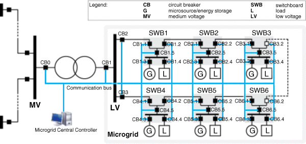
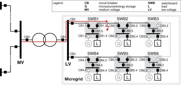
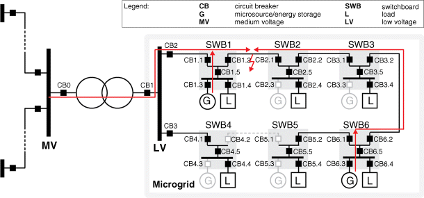
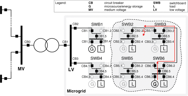
Figure 4.3 shows a typical microgrid comprising two feeders connected to the LV bus and to the MV bus via a distribution transformer. Each feeder has three switchboards (SWB). Each SWB has star or delta configuration and connects DERs and loads to the LV feeder. In the following, we analyze two external (F1, F2) and two internal (F3, F4) microgrid faults. All LV circuit breakers (from CB1 to CB6.5) may have different ratings but are equipped with a conventional over-current protection and are used for segmenting the microgrid.
Figure 4.3 External and internal fault scenarios in a microgrid
In general, protection issues in a microgrid can be divided in two groups, depending on the microgrid operating state (Table 4.1). The table also shows the importance of “3S” (sensitivity, selectivity and speed) requirements for different cases, which provides a basis for design criteria of a microgrid protection system.
Table 4.1 Major classes of microgrid protection problems
The next sections provide more details on each case of Table 4.1.
4.2.4 Grid Connected Mode with External Faults (F1, F2)
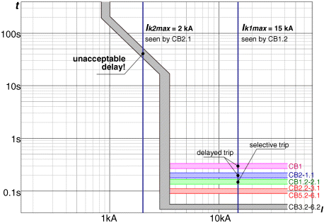
With fault F1, a main grid (MV) protection clears the fault. If sensitive loads are connected to the microgrid, it could have to be isolated by CB1 as fast as 70 ms (depending on the voltage sag level in the microgrid) [6]. Also, the microgrid has to be isolated from the main grid by CB1, in case of MV protection tripping failure. A detection of F1 with a generic OC relay can be problematic, in case most of the DERs in the microgrid are connected via PE interfaces with built-in fault current limitation (i.e. there is no significant rise in current passing through CB1). Typically, these units are capable of supplying 1.1 to 1.2*I DERrated (rated current of microgenerator) to a fault, unless the converters are specifically designed to provide high fault currents. This is much lower than a short-circuit current supplied by the main grid. A directional OC relay in CB1 is the only feasible solution, if current is used for fault detection. In order to increase relay sensitivity, the pick-up current setting is defined as the sum of fault current contributions from the connected DER units (4.1). DERs that have to be taken into consideration are the subset of units that contribute to the short-circuit current on the defined direction.
I rDER is the rated output current of a particular DER and kDER is its fault current contribution coefficient, set at 1.1 for PE interfaced DER and at 5.0 for synchronous DER units [7]. This value will vary for a large number of different types of DER. Thus, the setting has to be continuously monitored and adapted when microgrid generation undergoes changes (number and type of connected DER).
Alternatively, voltage sag (magnitude and duration) or/and system frequency (instantaneous value and rate of change) can be used as indicators for tripping CB1. It may be also required that the energy sources of the microgrid stay connected and supply reactive power to support the utility grid during the fault conditions. Depending on the particular grid code the duration of support depends on the level of residual voltage and may vary from a hundred milliseconds to several seconds.
With fault F2, the distribution transformer OC protection clears the fault by opening CB0. CB1 is opened simultaneously by a “follow-me” function (hardware lock) of CB0. On hardware lock failure, a possible fault sensitivity problem can arise as in the case of fault F1. Typical solutions are similar to the F1 case: directional adaptive OC protection, under-voltage and under-frequency protection and various islanding detection methods [8].
4.2.5 Grid Connected Mode with Fault in the Microgrid (F3)
With fault F3, microgrid protection must disconnect the smallest possible portion of the LV feeder by CB1.2 and CB2.1. CB1.2 is opened due to a high short-circuit current supplied by the main MV grid. If CB1.2 fails to trip, fault F3 must be cleared by CB1.1 which is a backup protection for CB1.2. However, the sensitivity of the OC protection relay in CB1.1 can be potentially disturbed, if a large synchronous DER (e.g. diesel generator) is installed and switched on at SWB1 (i.e. between CB1.1 and the fault F3). In this case, the fault current passing through CB1.1 with DER will be smaller than without DER, while the fault current at F3 will be higher due to additional DER contribution. This effect is known as protection blinding (the larger the synchronous DER the greater the effect – in some cases the fault current seen by CB1.1 can be reduced by more than 30%) and may result in a delayed CB1.1 tripping, because of the fault current transition from a definite-time part to an inverse-time part of the relay tripping characteristic (Figure 4.2). A delayed fault tripping will lead to an unnecessary disconnection of DER at SWB1 (usually low-power diesel generators have very low inertia and will run out of step in case of a delayed fault tripping). This issue can be solved by proper coordination of microgrid and DER protection systems. Another option is to adapt the protection settings with regard to current operating conditions (DER status).
If CB1.2 operates faster than CB2.1, which is very likely, it will island a part of the microgrid which will be connected to the fault F3. If it is possible to balance generation and load in the islanded segment of the microgrid (microsources are capable of supplying loads directly or after load shedding), it is expedient to isolate that group of microsources and loads from the fault F3 by opening CB2.1 and possibly closing CB3.2–6.2. However, a reversed and low-level short-circuit current in case of PE interfaced DER will cause a sensitivity problem for CB2.1 similar to the one described in the case of fault F1. Possible solutions include directional adaptive OC protection and a follow-me function of CB1.2, which opens CB2.1 (in this case, a communication failure may cause sensitivity problems for CB2.1).
4.2.6 Grid Connected Mode with Fault at the End-Consumer Site (F4)
With fault F4, a high short-circuit current is supplied to the fault from the main grid, together with a contribution from DER, which will lead to tripping of CB2.4. Frequently, there is a fuse instead of a CB, which is rated in such a way that a shortest possible fault isolation time is guaranteed. In case of no tripping, the SWB2 is isolated by CB2.5 and local DER is cut off. No sensitivity or selectivity problems are foreseen in this scenario.
4.2.7 Islanded Mode with Fault in the Microgrid (F3)
The microgrid might operate in islanded mode when it is intentionally disconnected from the main MV grid by CB1 (full microgrid) or a CB along the LV feeder (a segment of the microgrid). This operating mode is characterized by absence of the high short-circuit current supplied by the main grid. Generic OC relays should be replaced by directional OC relays, because fault currents flow from both directions to the fault F3. If CB1.2 and CB2.1 use setting groups chosen for the grid-connected mode, they will have a sensitivity problem with detecting and selectively isolating the fault F3 and tripping within acceptable time frame for PE interfaced DER (the fault current could shift from a definite-time part to an inverse-time part of the relay tripping characteristic). There are two possible ways to address this problem:
- Install a source of high short-circuit current (e.g. a flywheel or a super-capacitor) to trip CBs or blow fuses with settings or ratings for the grid-connected mode. However, a short-circuit handling capability of PE interfaces can be increased only by increasing the respective power rating or by having extensive cooling, which both lead to higher investment cost [9]. This solution is discussed in Section 4.4.
- Install an adaptive microgrid protection using online data about the microgrid topology and status of available microsources or loads. This solution is discussed in Section 4.3.
4.2.8 Islanded Mode and Fault at the End-Consumer Site (F4)
With fault F4, a low short-circuit current is supplied to the fault from the local DERs. There is no grid contribution to the fault current level. However, CB2.4 settings selected for the main grid-connected mode are just slightly higher than the rated load current. This ensures that the end-customer site will be disconnected, even if only PE-interfaced DERs are operating in the microgrid. If there is no tripping, the SWB2 must be isolated by CB2.5 using a directional OC relay. Similar to the grid-connected mode, there are no sensitivity or selectivity problems foreseen in the islanded mode for a fault at the end-consumer site.
4.3 Adaptive Protection for Microgrids
4.3.1 Introduction
As discussed in Section 4.2, time over-current protection is the most common method employed in MV and LV distribution grids, as it is quite simple to configure and is an economically attractive option. In networks with interconnected DER, short-circuit currents detected by over-current protection relays depend on the point of connection and the type and size (feed-in power) of the DER units. In these networks directions and magnitudes of short circuit currents will vary almost continuously, since the operating conditions in a microgrid are constantly changing due to the intermittent DERs (wind and solar) and periodic load variation. Also, the network topology can be regularly changed in order to achieve loss minimization or other economic or operational targets. In addition, controllable islands of different size can be formed, as a result of faults in the utility grid or inside a microgrid. In such circumstances coordination between relays may fail and generic OC protection with a single setting group in each relay may become inadequate, so it will not guarantee a selective operation for all possible faults. Therefore, it is essential to ensure that protection settings chosen for OC protection relays dynamically follow changes in grid topology and location, type and amount of distributed energy resources. Otherwise, unwanted or uncoordinated operation – or failure to operate when required – may occur. To solve the problems originating from the interconnection of DERs the protection relay settings can be adapted in a flexible way combined with the utilization of over-current protection relays with identification of current direction. Adaptation of settings could mean a continuous adaptation of relay characteristic settings or a switching of relay settings groups.
Adaptive protection is defined as “an online activity that modifies the preferred protective response to a change in system conditions or requirements in a timely manner by means of externally generated signals or control action” [10]. Technical requirements and suggestions for a practical implementation of an adaptive microgrid protection system, as seen by the authors, are:
- use of digital directional OC relays, since fuses or electromechanical and standard solid state relays (especially for selectivity holding) do not provide the flexibility for changing the settings of tripping characteristics, and they have no current direction sensitivity feature,
- digital directional over-current relays, which must provide the possibility for using different tripping characteristics (several settings groups, e.g. modern digital OC relays for LV applications have 2–4 settings groups) which can be parameterized locally or remotely, automatically or manually,
- use of new/existing communication infrastructure (e.g. twisted pair, power line carrier or radio) and standard communication protocols (Modbus, IEC61850, etc.), such that individual relays can communicate and exchange information with a central computer or between different individual relays quickly and reliably to guarantee a required application performance.
The communication time lag and the maximum time lag are not critical values for adaptive protection because the communication infrastructure is used to collect information about the microgrid configuration and to change accordingly the relay settings only prior to the fault. The interlock, if required, is done by means of physical point-to-point connection. On master–slave protocols like Modbus, the changes of configuration have to be identified with a maximum delay of 1–10 seconds depending on the dimensions of the network, and the protection system reconfiguration has to be completed in times of the same order, provided that basic backup protection functions are present during the transitory phase. On peer-to-peer protocols like IEC61850, the changes in the network configuration trigger protection reconfiguration. The accepted delays are equivalent to the previous ones.
The following sections present design of dynamic adaptive microgrid protection based on pre-calculated and “trusted” setting groups. An alternative design based on real-time calculated settings is also discussed. As with the microgrid energy management applications discussed in Chapter 2, the implementation of an adaptive protection system can be deployed with a centralized or decentralized approach, depending on the distribution of functionalities. Each approach requires a different communication architecture. The following sections focus on the centralized approach.
4.3.2 Adaptive Protection Based on Pre-Calculated Settings
The principles of a centralized adaptive protection system can be explained by the following example. Let's consider the microgrid of Figure 4.3, which includes a microgrid central controller (MGCC) and a communication system, in addition to primary switching equipment, as shown in Figure 4.4. The function of the MGCC can be carried out by a programmable logic controller (PLC), a station computer or a generic PC, located in a distribution secondary substation (MV/LV). Electronics make each CB with an integrated directional OC relay capable of exchanging information with the MGCC master–slave scheme, where the MGCC is a master and the CBs are slaves, via the serial communication bus RS-485 and using the standard industrial communication protocol Modbus [11]. By polling individual relays, the MGCC can read data (electrical values, status) from CBs and, if necessary, modify relay settings (tripping characteristics).
Figure 4.4 A centralized adaptive protection system
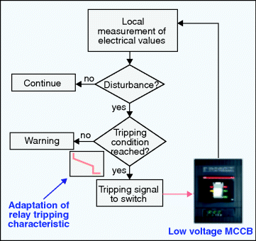
When a fault happens, each individual relay takes a tripping decision locally (independently of the MGCC) and performs in accordance with the algorithm shown in Figure 4.5. The main goal of the adaptation module is to maintain settings of each OC relay regarding the current state of the microgrid (both grid configuration and status of DERs are taken into consideration).
Figure 4.5 Local over-current protection function inside circuit breaker
The adaptation module in the MGCC is responsible for a periodic check and update of relay settings and consists of two main components:
- pre-calculated information during offline fault analysis of a given microgrid,
- an online operating block.
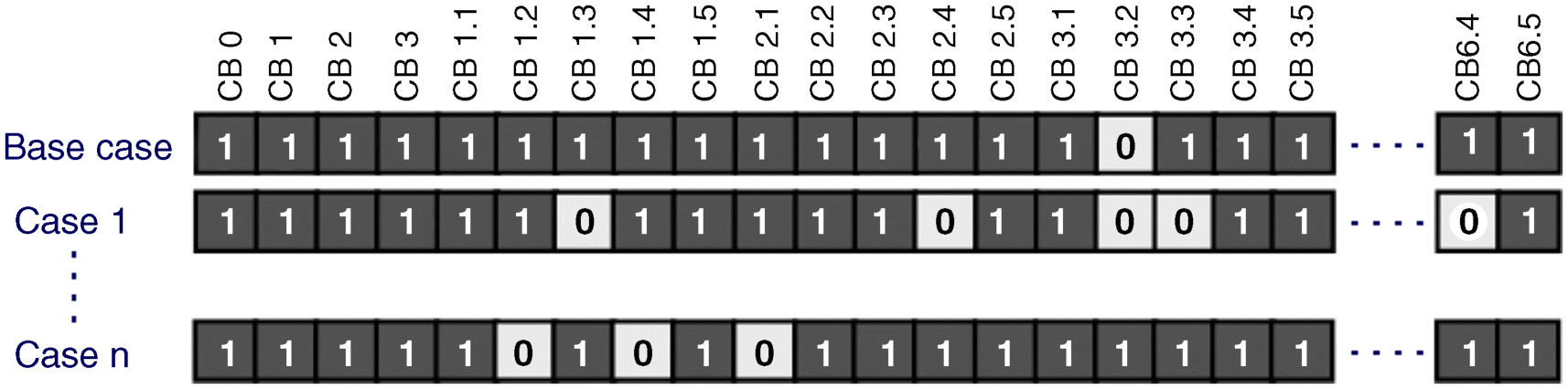
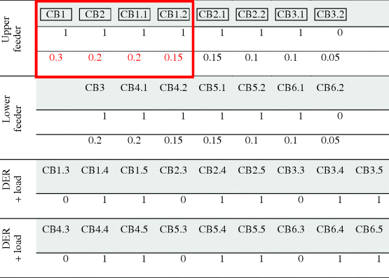
A set of meaningful microgrid configurations as well as feeding-in states of DERs (on/off) is created for offline fault analysis and is called an event table. Each record in the event table has a number of elements equal to the number of monitored CBs in the microgrid (some elements may have higher priority than others, such as the central CB which connects LV and MV grids) and is binary encoded, that is, element = 1 if a corresponding CB is closed and 0 if it is open (Figure 4.6).
Figure 4.6 Structure of the event table
Next, fault currents passing through all monitored CBs are calculated by simulating different short-circuit faults (three-phase, phase-to-ground etc.) at different locations of the protected microgrid at a time. During repetitive short-circuit calculations, the topology or the status of a single DER or load is modified between iterations. As different fault locations for different microgrid states are processed, the results (the magnitude and direction of fault current seen by each relay) are saved in a specific data structure.
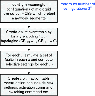
Based on these results, suitable settings for each directional OC relay and for each particular system state are calculated in a way that guarantees a selective operation of microgrid protection. These settings are grouped into an action table which has the same dimension as the event table. In addition to the regulation of protection settings, other actions such as activation of a protection function can be done, for example, a directional interlock can be activated in the islanding situation. The flow chart diagram of Figure 4.7 summarizes the offline part of the adaptive protection algorithm.
Figure 4.7 Steps of the offline adaptive protection algorithm
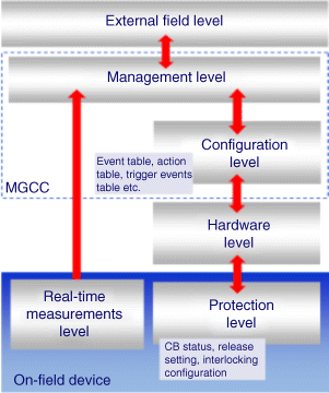
The event and action tables are parts of the configuration level of the microgrid protection and control system, as shown in Figure 4.8:
- External field level represents energy market prices, weather forecasts, heuristic strategy directives and other utility information.
- Management level includes historic measurements and the distribution management system (DMS).
- Configuration level consists of a station computer or PLC situated centrally (substation) or locally (switchboard) which is able to detect a system state change and send a required action to hardware level.
- Hardware level transmits a required action from the configuration level to in-field devices by means of a communication network. In the case of a large microgrid, this function can be divided between several local controllers that communicate only selected information to the central unit.
- Protection level may include information, such as CB status, release settings and interlocking configuration. Together with the real-time measurements level they are residing inside in-field devices.
Figure 4.8 Microgrid protection and control architecture
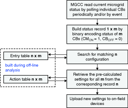
During online operation, the MGCC monitors the microgrid state by polling individual directional OC relays. This process runs periodically or is triggered by an event (tripping of CB, protection alarm etc.), as shown in Figure 4.9. The microgrid state information received by the MGCC is used to construct a status record that has a similar dimension to a single record in the event table. The status record is used to identify a corresponding entry in the event table. Finally, the algorithm retrieves the pre-calculated relay setting groups from the corresponding record in the action table and uploads the settings to in-field devices via the communication system. Alternatively, it may send commands to protection devices in the field, to switch between setting groups pre-loaded in the memory of these devices during system configuration.
Figure 4.9 Steps of online adaptive protection algorithm with available look-up tables (event and action tables)
The following examples illustrate the operation of the centralized adaptive protection system described in the previous paragraphs.
4.3.3 Microgrid with DER Switched off, in Grid-Connected Mode
The microgrid topology of Figure 4.10 is used as a base case and provides the first entry in the event table. The following Table summarizes its electrical characteristics.
| Parameters of utility grid | Value |
| Rated voltage, V | 6000 |
| Short-circuit power, MVA | 500 |
| Parameters of distribution transformer | Value |
| Rated voltage primary/secondary, V | 6000/400 |
| Rated power, kVA | 630 |
| Vcc, % | 4 |
| LV distribution system | TN-S |
| Parameters of cables | Value |
| TYPE | EPR/XLPE |
| Cross-section phase, mm2 | 3 × 185 |
| Cross-section neutral, mm2 | 95 |
| Nominal current, A | 750 |
| Resistance at 20 °C phase/neutral, mΩ | 8.34/16.24 |
| Inductance at 20 °C phase/neutral, mΩ | 6.17/6.25 |
| Length, meters | 150 |
| Parameters of feeder circuit breakers | Value |
| Rated voltage, V | 400 |
| Rated current, A | 800 |
| Parameters of loads | Value |
| Rated voltage, V | 400 |
| Rated current, A | 100 |
| Rated power factor, cosφ | 0.9 |
| Parameters of synchronous DERs | Value |
| Rated voltage, V | 400 |
| Rated apparent power, kVA | 160 |
| Rated power factor, cosφ | 0.8 |
| Direct-axis sub-transient reactance Xd″, % | 9.6 |
| Quadrature-axis sub-transient reactance Xq″, % | 10.2 |
| Direct-axis transient reactance Xd′, % | 21 |
| Direct-axis synchronous reactance Xd, % | 260 |
| Negative sequence reactance X2, % | 9.8 |
| Zero sequence reactance X0, % | 2.1 |
| Direct-axis sub-transient short circuit time constant Td″, ms | 11 |
| Direct-axis transient short circuit time constant Td′, ms | 85 |
Figure 4.10 Scenario A1: the microgrid with DERs switched off, connected to the MV distribution grid
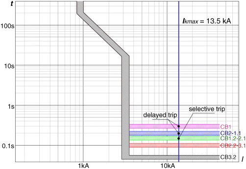
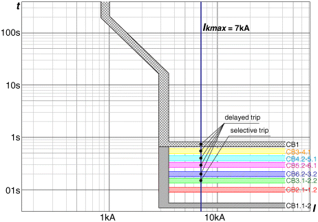
We assume that each protection device has a similar shape to the over-current protection trip curve (Figure 4.2). In order to provide a selective operation of different circuit breakers, we used different time delays t s of the constant time delay part S in the range between I kmin (the expected minimum short-circuit current) and I kmax (the expected maximum short-circuit current). CB1 is the closest circuit breaker to the source and has the longest time delay t s. The most distant, CB3.2 and CB6.2, have the shortest time delay t s (Figure 4.11). The instantaneous tripping part, I, is removed from all curves as a simplification.
Figure 4.11 Trip curves for circuit breakers in the upper feeder (identical for CBs in the lower feeder) in the base case and a tripping sequence in scenario A1
The microgrid topology and suitable OC protection settings t s for all CBs (calculated during the offline fault analysis [12]) in the base case are shown in Table 4.2, based on Figures 4.10 and 4.11. DER and load protection settings are not set here, but the information on DER and load status (on/off) is required for correct operation of the microgrid adaptive protection.
Table 4.2 Scenario A1 – status of circuit breakers: 1 = close, 0 = open and over-current protection settings t s in seconds. Box and numbers show CBs that see the fault in Figure 4.10.
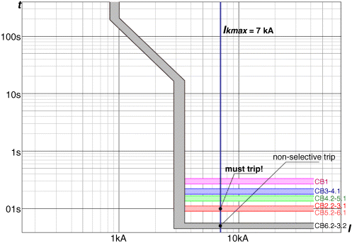
In case of a fault in the cable between SWB1 and SWB2 (Figure 4.10) all CBs between the fault and the LV busbar see the fault current supplied by the main MV grid (box in Table 4.2), but only CB1.2 will trip after t s = 150 ms (Figure 4.11), and CB2.1 will be opened by the follow-me function of CB1.2, in order to avoid connecting the fault to the healthy feeder by closing CB3.2 and CB6.2. Other CBs that see the fault are delayed (in absence of a logic discrimination auxiliary connection). However, this method is limited by a number of discriminating time steps (a maximum t s is recommended to be less than 800 ms) and is only suitable for feeders with a small number of switchboards.
If we assume that SWB2 and SWB3 are resupplied via SWB6 (CB3.2 and CB6.2 are closed) after the fault between SWB1 and SWB2 is selectively eliminated (CB1.2 and CB2.1 are open) a selectivity problem may appear if we use the base case protection settings of Table 4.2.
For example, if the second fault appears between SWB2 and SWB3 (Figure 4.12), it will be eliminated by CB3.2 and CB6.2 (t s = 50 ms) instead of CB3.1 (t s = 100 ms) and the load in SWB3 will be unnecessarily tripped as shown in Figure 4.13.
Figure 4.12 Scenario A2: the microgrid with all DERs switched off, connected to the MV distribution grid
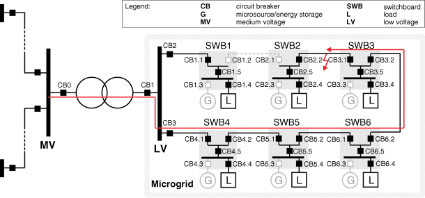
Figure 4.13 Base case trip curves and a tripping sequence in scenario A2 with non-directional OC protection
Selectivity can be improved by:
- application of directional over-current relays,
- modification of protection settings of non-directional OC relays.
In the case of directional over-current protection, each relay will have two t s settings, one in each direction (clockwise and counter-clockwise, or forward and backward), as shown in Table 4.3. In this case a selective protection operation is guaranteed (Figure 4.14) and SWB3 will remain connected after the fault is eliminated.
Table 4.3 Scenario A2: Status of CBs and directional OC protection settings t s
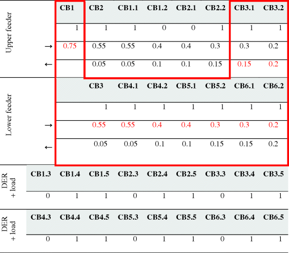
Figure 4.14 Base case trip curves and a tripping sequence in scenario A2 with directional OC protection
In the second case, we modify the S part of the base case trip curves by adjusting t s settings (Figure 4.15). Second records in the event and action tables are created during the offline fault analysis (Table 4.4).
Figure 4.15 Modified base case trip curves (ts settings) and a tripping sequence in scenario A2 with non-directional OC protection
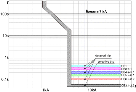
Table 4.4 Scenario A2: Status of CBs and modified non-directional OC protection settings t s
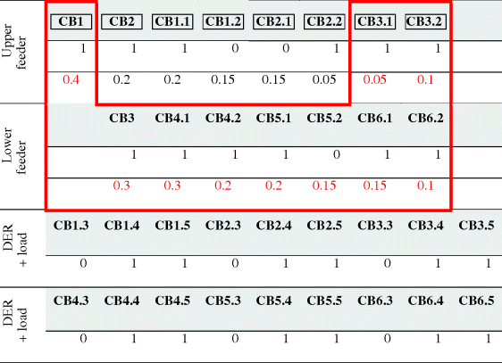
In particular, we can observe lower t s for CB2.2 and CB3.1 and higher t s for CB3.2 and CB6.2, in comparison to the values shown in Table 4.2.
The second solution with a modification of t s settings is characterized by a narrower range of the time delay t s. The maximum time delay t s is 0.4 s as opposed to 0.75 s in the case of directional OC protection.
4.3.4 Microgrid with Synchronous DERs Switched on in Grid Connected and Islanded Modes
Assume that there is a considerable change in the microgrid configuration and status of DER units: the cable between SWB4 and SWB5 is disconnected for a maintenance work and SWB5 and SWB6 are supplied via SWB3 (CB3.2 and CB6.2 are closed) as illustrated in Figure 4.16. Two identical synchronous diesel generators are connected at SWB1 and SWB6. In addition, we assume that all non-directional OC protection relays use time delay settings t s from the base case shown in Table 4.2.
Figure 4.16 Scenario B1: the microgrid with synchronous DERs connected to the MV distribution grid
In the case of fault between SWB1 and SWB2 (Figure 4.16) there is no problem in detecting and selectively isolating the fault from the main grid side by CB1.2, because the fault current seen by CB1.2 becomes higher I kmax = 15 kA (Figure 4.17) than 13.5 kA (Figure 4.11) in the base case due to a contribution from the synchronous DER at SWB1. The fault current supplied by the second DER at SWB6 and seen by CB2.1 is 2 kA (Figure 4.17). It can only activate the L part of the relay's trip curve with the expected tripping time delay of 40 s. Therefore, CB2.1 is opened by the follow-me function of CB1.2 and isolates the fault from the LV feeder side in t s = 150 ms (if using a directional OC protection then t s = 400 ms, see Table 4.3).
Figure 4.17 Base case trip curves and a tripping sequence in scenario B1 with directional OC protection
The main concern is t s ≥ 150 ms set for the OC relay in CB1.2, which may affect the stability of the synchronous DER with a small inertia at SWB1. A preferred solution is based on the adaptive directional interlock. The time delay t s is set at 50 ms for all OC relays in the microgrid. Then blocking signals are sent in the correct directions, which prevents an unnecessary disconnection of DERs and healthy parts of the microgrid.
Next we assume that, after an isolation of the first fault, the island which includes SWB2, 3, 5 and 6 is formed as shown in Figure 4.18. The synchronous DER in SWB6 is switched to a frequency and voltage control mode, and additionally each load in the island is reduced from 100 A to 50 A.
Figure 4.18 Scenario B2: the islanded microgrid with the synchronous DER in SWB6
Assume that there is a second fault inside the islanded microgrid between SWB2 and SWB3 and all non-directional OC relays use t s settings from the base case shown in Table 4.2. Ideally, the fault should be cleared by CB2.2 and CB3.1. CB2.2 can not trip since there is no fault current source at SWB2, but it can be opened by the follow-me function of CB3.1. The t s of CB3.1 is set at 100 ms for a minimum fault current level of 4*I n CB = 3.2 kA. In case of using directional OC protection, then t s = 150 ms for CB3.1 (Table 4.3). However, the maximum fault current supplied by the synchronous DER at SWB6 and seen by CB3.1 is I kmax = 2.4 kA (Figure 4.19). This will activate the L part of the relay's trip curve with the expected tripping time delay of 25 s. During this time, the DER at SWB6 will be disconnected by its out-of-step protection.
Figure 4.19 Base case and modified trip curves and a tripping sequence in scenario B2
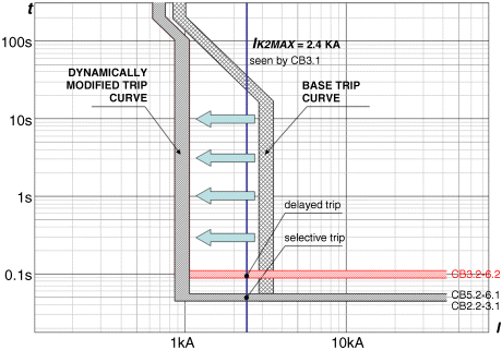
In order to guarantee fast fault isolation in the islanded mode where the main grid does not contribute to the fault, the trip curve must be pushed to the left dynamically, depending on the microgrid topology and a number of connected DERs. The modified trip curves for scenario B2 are illustrated in Figure 4.19.
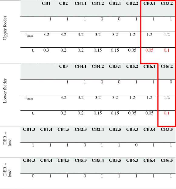
Protection settings for all CBs in the island are calculated during the offline fault analysis and shown in Table 4.5, as recorded in the event and action tables.
Table 4.5 Scenario B2: Status of CBs and modified OC protection settings I kmin and t s
Another protection alternative is based on the adaptive directional interlock. The tripping time is set at 50 ms for all CBs inside the island, and the minimum short-circuit current has to be dynamically modified (reduced) depending on the type and number of connected DER units.
A more elaborate example of multilevel microgrid and centralized adaptive protection system is provided in the Appendix 4.A.1.
4.3.5 Adaptive Protection System Based on Real-Time Calculated Settings
An alternative centralized approach to the one based on predefined settings is to recalculate protection settings in real-time operation, immediately upon changes in the microgrid topology (network reconfiguration or DER connections). This protection scheme can be implemented as a multifunctional intelligent digital relay (MIDR). When a fault occurs, the routine implemented in the MIDR generates selective tripping signals, which are sent to respective circuit breakers. The MIDR allows continuous real-time measurement and monitoring of the analog and digital signals originating from equipment and network, respectively. Integration of state estimation routines into a configuration of the protection system, which monitors the DER operating state and sets up a corresponding data exchange with the protection system is also possible [13]. Thus, new network operating conditions can be assessed, functioning of the protection system can be analyzed and, if required, protection settings can be adapted. Figure 4.20 illustrates the algorithm of the developed adaptive protection relay. The scheme consists of two blocks: real-time and non-real time.
Figure 4.20 Simplified flow chart of adaptive protection system concept
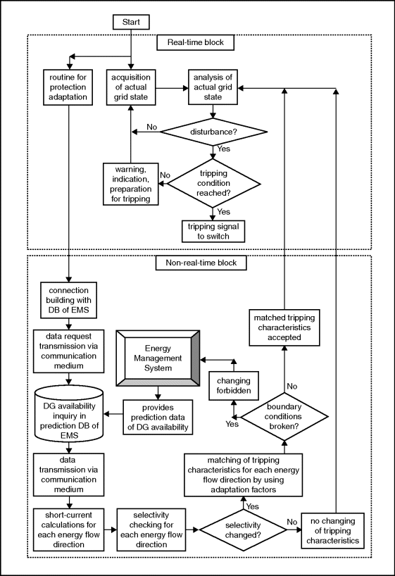
The real-time block analyzes the actual microgrid state, acquired by continuous measurement of microgrid parameters, and detects disturbances due to adjusted tripping characteristics of protection devices. When a tripping condition is detected, a tripping signal to the respective circuit breaker is generated by the MIDR. The non-real-time block uses the prediction data of the availability of DERs in order to review the selectivity of the tripping characteristics for each new operating condition and to adapt them accordingly, if selectivity is not suitably provided any longer. If the adaptation is successful and the boundary conditions are not violated, the tripping characteristics of respective relays will be matched. If there is no possible solution without violating the boundary conditions, a signal will be generated that forbids the acceptance of the operation predicted by the (decentralized) energy management system (DEMS/EMS).
The proposed adaptive protection concept for microgrids with protection settings calculated online was tested and proved in the 10/0.4 kV simulator in the laboratory of Fraunhofer IWES (Figure 4.21). The simulator is equipped with photovoltaic systems, combined heat and power units, diesel generators, models of wind power plants and different types of inverters.
Figure 4.21 Structure and primary equipment of 10/0.4 kV simulator in DeMoTec laboratory at Fraunhofer IWES
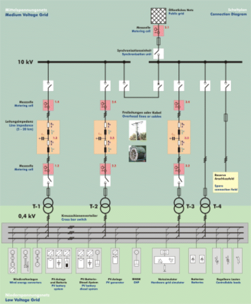
In the test setup, the MIDR comprises the functionalities of both DEMS and MV/LV station controller. For each of the three feeders (transformers T-1 to T-3), there is a separate database server, realized by means of MySQL servers. In the databases, data about the interconnected distributed energy resources (i.e. available short-circuit power provided by DER units) and the actual microgrid configuration is stored. The actual interconnection states and short-circuit power of DER units are stored in the respective databases and continuously communicated to the MIDR. Communication between the MIDR and the database servers can be realized via PLC or Ethernet. Based on the requested operational data (short-circuit power of DER in the different grid sections) and the actual short-circuit power available from the main grid, the MIDR calculates possible short-circuit currents and adapts the protection settings, where required. According to the protection characteristics and the measurement signals supplied by the current and voltage transformers, the MIDR decides whether there is a fault or not, and sends tripping signals to respective circuit breakers, if required. In this concept, the MIDR plays the role of the centralized protection controller which limits its application to a single substation case. For remote circuit breakers, communication can become a bottleneck for fast fault detection and isolation and will require the presence of reliable high-bandwidth communication channels.
Results from the tests are shown next. On the LV side of the transformer T-1, a synchronous generator is connected, which is able to feed the loads of the microgrid for islanded operation. At the LV side of the transformer T-3, an inductive motor with I rated = 50 A is connected. This value is indicated in the two current-time protection diagrams by means of a white line (Figure 4.22).
Figure 4.22 I–t protection diagrams for the feeder 3 (T-3) for the grid connected (left) and the islanded (right) operation modes
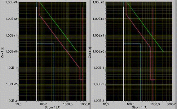
The diagrams of Figure 4.22 show the MIDR protection settings I (t) at the Feeder 3 for the grid connected (left) and the islanded (right) operating conditions. The bottom line shows the simplified motor startup characteristic, the top line indicates the short-circuit characteristic (damage curve) of the LV cable installed between the motor and the transformer T-3 and the middle curve is the tripping characteristic of Feeder 3, which controls the operation of the circuit breaker at the LV side of transformer T-3. The tripping curve is set between the motor startup characteristic and the damage curve of the LV cable. Its high set element (I ![]() ) is set to 0.8 times the maximum available short-circuit current.
) is set to 0.8 times the maximum available short-circuit current.
For the grid connected operation the maximum available short-circuit current at the Feeder 3 is 3700 A, which is indicated by the vertical line. Therefore, I ![]() (right part of the middle line) is set to 0.8 × 3700 A = 2960 A for the grid-connected operation. For the isolated operation (full short-circuit power is provided only by local DER) the maximum available short-circuit current at Feeder 3 is reduced more than four times to 800 A. Therefore, I
(right part of the middle line) is set to 0.8 × 3700 A = 2960 A for the grid-connected operation. For the isolated operation (full short-circuit power is provided only by local DER) the maximum available short-circuit current at Feeder 3 is reduced more than four times to 800 A. Therefore, I ![]() is now set to 0.8 × 800 A = 640 A. The MIDR automatically adapts the protection settings in accordance with the conditions of the microgrid. When a fault occurs in the microgrid, the middle line is exceeded and tripping signals are generated by the MIDR in order to trip the respective circuit breaker(s). The MIDR then behaves like a conventional protection relay which controls more than one circuit breaker.
is now set to 0.8 × 800 A = 640 A. The MIDR automatically adapts the protection settings in accordance with the conditions of the microgrid. When a fault occurs in the microgrid, the middle line is exceeded and tripping signals are generated by the MIDR in order to trip the respective circuit breaker(s). The MIDR then behaves like a conventional protection relay which controls more than one circuit breaker.
Similarly to the example above, during transition from grid-connected to islanded operation, the protection settings will be adapted for a change in the interconnected DER (i.e. a change in short-circuit contribution provided by DER), since some DERs will be left up-stream of the point of connection. The MIDR continuously monitors the DER availability (relevant data available from database servers) and the main grid availability (if applicable) and estimates the short-circuit currents for every short-circuit flow direction. The vertical line of the above diagrams, which indicates the estimated short-circuit current, is shifted accordingly and the curve adapts to the new conditions. The speed of protection adaptability is limited by the probability of fault occurrence during adaptation. During the tests carried out, the time duration for adaptation has been estimated to be in the range of a few seconds.
The suggested adaptive protection concept does not consider the function of automatic reclosing, which is usually employed for temporary faults occurring on overhead lines. Of special relevance to this concept is the data transfer between adaptive relays and EMS over long distances. Communication via power line carrier (PLC) and LAN is a preferred option. For a practical implementation, wireless radio communication should be considered for long distance communication.
For the implementation of the adaptive network protection concept in distribution networks, existing communication systems and protocols can be applied. The IEC 61850 standard allows for real-time communication by means of periodically sent telegrams. For a sudden change of state at the sending unit, a telegram (GOOSE message = Generic Object Oriented Substation Event) will be send with a high repetition rate within a few milliseconds after the change of state. Thus, changes in the microgrid state can be detected rapidly. The communication link can be established by means of common interfaces (RS-485, fiber optic etc.) and protocols. Communication architectures and protocols are discussed in Section 4.3.6.
4.3.6 Communication Architectures and Protocols for Adaptive Protection
As explained in the previous sections, the implementation of an adaptive protection system requires that protection intelligent electronic devices (IEDs) communicate between themselves or with a central controller. By these communications, IEDs can provide and receive information about the actual topology of the microgrid, about the status of generators, energy storage devices and loads, and commands to execute an action (e.g. change of the active setting group). The application of pre-calculated protection settings, can be deployed via a centralized or a decentralized communications architecture:
- A centralized architecture is the most conventional and common communication scheme. There is a central controller that takes decisions about protection IEDs which have different settings for different operating conditions. This architecture is supported by many communication protocols, the most common ones within the electric energy sector being: Modbus, DNP3, IEC 60870-5-101/104 and IEC 61850. The centralized architecture can be deployed with serial communications, bus communications, over PLC or through an Ethernet network.
- A decentralized architecture is less conventional. Within this architecture it is not necessary to employ a central controller that coordinates protection settings, because intelligence is distributed between IEDs themselves. Each IED, with the information received from other IEDs, acts autonomously in order to change its active setting group. This architecture is only feasible when the communication protocol allows it to establish a direct communication between the IEDs, substituting direct hardwired connections between the relays. For standard protocols, today the industry's focus is on IEC 61850. The decentralized architecture needs to be implemented over a bus or Ethernet network, although with a suitable bandwidth it can be implemented with future 4G wireless networks or over PLC.
The most significant advantage of a centralized architecture is that local protection devices do not take decisions and therefore they are simpler. The central controller processes data and makes decisions based on the data received from the local devices. For example, to implement an adaptive protection system, the programmable logic is solely run on the central controller. It receives information about the status of all switching devices (feeder, DERs and loads) from local protection devices, such as IEDs. After the decision is taken, the central controller sends setting switching commands to the corresponding IEDs. The main disadvantage of a centralized architecture is its full dependence on the central device. Failure of this central element means total loss of the adaptive protection system, so redundancy is needed, which means additional cost.
The biggest advantage of the decentralized architecture is that it does not depend on one central controller. Its biggest disadvantage is the requirement for more advanced local protection devices, since each local device will need to run dedicated programmable logic for autonomous adaptation of settings depending on microgrid operating conditions.
Regarding the communication protocols that enable a protection system to become adaptive, the IEC 61850 standard receives most interest. Its main disadvantage is that it requires an Ethernet network. Ethernet is a common technology for automation at HV and MV (the previous section covered adaptive protection based on IEC 61850), but today, it still means extra cost and technical complexity in LV installations. Moreover, it poses additional complexity for the maintenance personnel, who are more familiar with hardwired systems.
The main advantages of IEC 61850 are:
- can be applied to every type of electrical installation and is able to functionally cover any application,
- guaranteed interoperability between devices from different vendors,
- standardized data models,
- simplified engineering process and IED configuration,
- scalable solutions.
For adaptive protection application, this standard has communication services for the usual operations within electrical installations, such as change of settings and setting groups, reporting of information, commands and so on. One remarkable service is the GOOSE (generic object oriented substation event) service, already mentioned in Section 4.3.5. This service makes direct information exchange between IEDs possible, accepting any type of data (single signals, double signals, measurements etc.), guaranteeing that it is transmitted in less than 3 ms (faster than a cable between digital outputs and inputs), and is always available because it is retransmitted indefinitely. It comprises a multi-master system that offers the highest reliability. Obviously, the application of GOOSE messages for communication between IEDs within the microgrid, provides a valuable tool allowing them to adapt their configurations to any operational scenario. Each IED can receive data from all the others very rapidly, so the reconfiguration process is very fast.
Figure 4.23 shows an example of how the GOOSE messaging can be used in a microgrid. A protection IED at the LV side of the distribution transformer in bay 1C issues a signal to block the trip of protection IEDs within the microgrid in bays 1A, 1B, 1D and at the IED immediately on the LV side of the transformer. Protection IEDs on those bays need only subscribe to that GOOSE message in order to effectuate the blocking scheme. GOOSE messages can be used to inform other IEDs about topological changes in a microgrid (e.g. transition from grid connected mode to islanded mode), to implement protection schemes (like the one in Figure 4.23), to execute commands (e.g. open/close circuit breakers), to change active setting group and so on.
Figure 4.23 The blocking scheme based on GOOSE for faults in the microgrid

An adaptive protection system, such as one designed according to the IEC 61850 standard, requires higher investment than a traditional protection system for LV based on fuses and hardwired interlock. However, microgrid operation will not be feasible without an adaptive protection system. Perhaps one of the main concerns in considering the IEC 61850 solution is the cost of the network, especially the cost of devices that were not necessary in traditional LV networks, the “switches”. Switches enable the organizing of the traffic within the network, taking into consideration several parameters, such as the priority of a message, or managing VLANs in order not to mix different traffics. Switches are necessary, but it is possible to use cheaper architectures by means of integrating these switches inside IEDs. The implementation of an Ethernet network as a single ring of IEDs with integrated switches is a very good option in order to reduce the cost of a high-performance microgrid.
4.4 Fault Current Source for Effective Protection in Islanded Operation
As discussed in Section 4.1, one of the major problems in microgrid protection is the low contribution to faults by DERs that have power electronics (PE) interfaces. This section analyzes the installation of an independent system that supplies a fault current in the microgrid dominated by DERs with PE interfaces, for example, PV panels. The proposed system, designed as a fault-current source (FCS), is based on power electronics but uses a simpler and thus less costly technology than is normal in inverters in this power range. An FCS would consist of the following subsystems:
The operating principles of an FCS are illustrated in Figure 4.24. Its power circuit remains idle during normal operation of the network (1). Whenever a fault occurs, the network voltage drops (2), the FCS is activated (3) and it attempts to restore the original network voltage, thereby injecting a fault current into the network. The FCS has finite impedance and, as a consequence, the voltage could be lower than the nominal voltage of the network. The current is high enough to cause a fuse or circuit breaker to clear the fault. Subsequently, the FCS maintains the original voltage and frequency (4), to enable inverters that had turned off to resynchronize and reconnect to the network. After some time, typically 5 seconds, the FCS can turn off because the full load is now supplied by the local sources in the microgrid.
Figure 4.24 Typical voltage waveforms illustrating the operation of an FCS
In most LV networks, there is a statutory requirement to detect and remove a low-impedance fault within a few seconds, for example 5 seconds. Therefore after 5 seconds the FCS can assume that the fault has been cleared and that it is justifiable to cease operation. However, this should not happen instantaneously, because some sources in the microgrid may have switched off as a consequence of the voltage dip during the fault and need some time to reconnect. Therefore, at the end of the 5 second interval, the FCS will remain operating, while gradually increasing its virtual impedance, and then cease operation. Once triggered, the FCS acts like a low-impedance voltage source. The most sensible location for an FCS in a microgrid is therefore the main LV distribution busbar of the distribution step-down transformer, if the microgrid is normally supplied from an MV network. In this way, a classical radial topology is possible with straightforward graded protection settings along individual feeders. In order to avoid a misoperation of the protections in the network, it is recommended to always install DERs, whose fault current contribution is much smaller than the fault level created by the FCS at the first protection device upstream of the DER. If the decision to install a DER is beyond the authority of the network operator, the available DERs have to be taken into account when setting the protections.
In order to demonstrate the operating principle of FCS, a single-phase prototype with the following specifications has been used:
| Network voltage | 230 V single-phase |
| Maximum fault current | 200 A rms |
| Energy storage technology | ultra-capacitors |
| Capacitance of UC stack | 0.44 F |
| ESR of UC stack | 2.3 Ω |
| Maximum voltage of UC stack | 840 VDC |
The FCS would require a minimum voltage of ∼585 VDC to be able to restore the network voltage to a value within statutory limits. This means that the energy effectively available to be injected into the network is 80 kJ. The effective series resistance (ESR) of the ultra-capacitor limits the amount of power that can be delivered by the FCS. If a voltage drop of 20% of the maximum voltage is accepted, the maximum DC discharging current is 73 A and the maximum DC power to be delivered is 49 kW. Technical details of the construction of the FCS and its control logic are provided in Appendix 4.A.2.
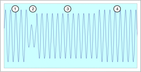
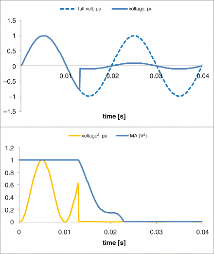
Failure of a network to trigger a thermal fuse can be considered as a failure to deliver the required amount of energy as soon as a fault occurs. For this reason, the fault detection algorithm uses the thermal value of the voltage (the squared value) as a variable to monitor. The squared value of a 50 Hz sinusoidal voltage varies sinusoidally at a frequency of 100 Hz. An accurate measurement of the thermal value therefore involves averaging over an integer number of half-periods. The quickest way to observe changes in the thermal value is by using a moving average of the squared voltage over one half-period. The speed of response of the detection depends on the threshold that is applied. A reasonable upper value of the detection threshold corresponds to 80% of the rated voltage. In this way, the system will never respond to small transients even if the stationary grid voltage is on its lower statutory limit of 90%. The 80% corresponds to a threshold 64% (0.82) for the moving average of the squared voltage. A collapse of the voltage to 10% is detected within 2 ms, as shown in Figure 4.25.
Figure 4.25 Dip of the grid voltage to 10% from T = 0.013 (upper traces), squared grid voltage and moving average of V2 over one half-period (lower traces)
Laboratory tests from the operation of the prototype in parallel to a utility power supply with additional high series impedance are presented next. The circuit diagram is shown in Figure 4.26. Some of the tests have been done using a standard D type thermal fuse, as depicted in the diagram. Other tests have been performed using an automatic circuit breaker with thermal/magnetic operation. The 7 Ω impedance in series with the supply ensures that a short circuit, as indicated in the diagram, will lead to a fault current of ∼30 A, which is too low to trigger either the fuse or the circuit breaker within 5 seconds.
Figure 4.26 General test setup, demonstrating the functionality of the FCS
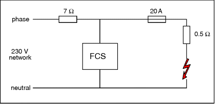
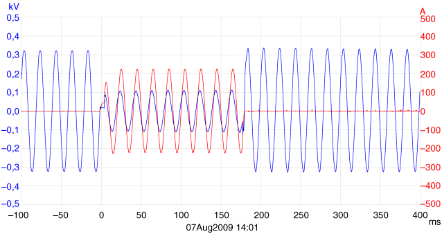
Figure 4.27 depicts the voltage across the FCS and the current through the short circuit. The fuse at the end consumer premises blows after 180 ms. In the particular configuration of this prototype, the FCS is able to blow thermal fuses up to 35 A. If larger fuses need to be blown, the required energy will scale more or less linearly with the required current. As energy content is the main cost driver of an FCS, an FCS capable to blow, for example, a 200 A fuse would be six times bigger and six times more expensive than the prototype.
Figure 4.27 Voltage across the FCS (zero before and after event) and current through the short circuit (larger sinusoid during the event). Protection device: fuse DII 20 A
4.5 Fault Current Limitation in Microgrids
Distribution utilities calculate fault current levels during the network planning stage to ensure that fault levels remain within the design limits of various grid components. These calculations are based on knowledge about connected generating units and rotating equipment at customer sites. In today's distribution networks, the presence of DERs provides an additional contribution to the fault level, and the embedded nature of the DERs makes the fault current calculations more complex, as they should take into account the consequences of operational combinations to a degree not required when all generation is coming from the transmission network [7]. Even if the fault current contribution from a single DER is not large, the aggregated contribution of many DERs can raise the fault current levels beyond the design limits of various equipment components (e.g. circuit breakers, cables, busbars etc.). When the fault level design limits are exceeded, there is a risk of damage to, and failure of, the equipment, with consequent risks of injury to personnel and interruption of supply under short-circuit fault conditions. In this case, a costly upgrade of equipment may be needed.
The fault level contribution from a DER is mainly determined by its type and its coupling method to the grid. Today, DERs connected to LV microgrids are commonly PV generators and micro and mini CHPs. Existing LV microgrids can accept a large number of PV generators. The impact of PV covering 100% of the microgrid load would add less than 5% to the commonly used fault levels. However, for large numbers of domestic mini CHPs equipped with synchronous generators, fault currents may increase considerably, especially in urban areas with low fault-level headroom availability (a fault current level with DER can reach 130–150% of the fault current without DERs). In such circumstances the capability of a microgrid to accommodate additional DER units is reduced.
The duty of a fault current limiter (FCL) is to limit the excessive currents, in the case of a fault. The current-limiting effect is illustrated in Figure 4.28. In case of fault, the fault current increases with a certain rate of rise, depending on the circuit parameters and the phase angle at fault initiation. Usually, the FCL has to react and limit the current before the first peak of the fault-current waveform is reached (<5 ms). Figure 4.29 demonstrates available and emerging technical solutions for current limitation below equipment design limits [14]. These solutions fall in two groups: passive and active.
Figure 4.28 The effect of a fault current limitation
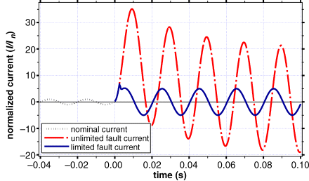
Figure 4.29 Alternative methods of fault current limitation
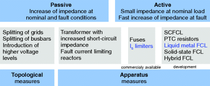
Passive solutions limit the fault current by increasing its current path impedance at nominal and post-fault conditions. Therefore, it generates losses and a voltage drop under nominal conditions. Active devices exhibit a highly nonlinear behavior and quickly increase the impedance during the fault. Their main disadvantage is the need to replace them after each operation and a careful adjustment of the protective relay settings to maintain selectivity [15]. There are also LV circuit breakers available with a built-in current limiting functionality [11]. The current limitation is done by a sufficient voltage build-up inside the breaker. The current path inside a CB is constructed in such a way that magnetic forces quickly move the arc into a set of metallic plates, making the arc split into a number of smaller arcs, each causing a voltage drop of 20–30 V and limiting the fault current [16]. However, the current limiting circuit breakers only limit the current in case of actuation and always interrupt. Selectivity is therefore limited.
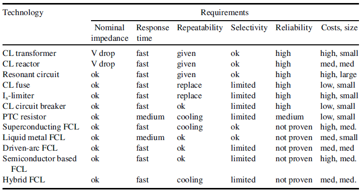
CIGRE WG A3.10 [14] provides a list of requirements for the ideal FCL:
- negligible impedance under nominal operating conditions – that is, negligible resistive and reactive losses, no related needs for cooling and no voltage drop;
- fast response – the first peak of the short-circuit current (<5 ms) must be limited in order to limit the magnetic forces on the primary equipment components;
- multiple operations – the FCL device has to recover automatically, with very short recovery time in order to be able to respond to multiple re-closure cycles and in order not to require a field trip for service personnel to replace components after operation;
- selectivity – the let-through current should be selectable, either by the design of the FCL device or by a configurable setting. It should not limit motor start currents and should not respond to transients or capacitor switching currents. The current for coordination with protective devices has to be provided, so that existing protection concepts do not need to be modified;
- high reliability – the FCL must correctly operate under any fault magnitude and any fault phase condition. Correct response must reliably occur after a long duration without fault events as well as in cases of consecutive multiple faults;
- compact size, long lifetime, maintenance free and low cost.
In Table 4.6, compliance with the requirements of the ideal FCL is given for different technologies.
Table 4.6 Compliance of different technologies with the requirements for the ideal FCL
A device called an Is-limiter combining a fast switch and a current limiting fuse in parallel (Figure 4.30) has been developed [17]. Under normal operation the current flows via the low impedance switch. Upon detection of a fault current by the electronic control circuit, the fast switch is triggered and the current is commutated to the fuse. By using a small charge for interrupting the main current path, the Is-limiter is able to interrupt the fault current within 0.5 ms after receiving the tripping signal. Due to the electronic control the tripping conditions can selectively be chosen. The Is-limiter is a single-shot device, and the switch/fuse insert needs to be replaced after actuation. Is-limiters are available for up to 40.5 kV and for rated currents of several kA.
Figure 4.30 Is-limiter with insert (a) and its current limiting effect (b)
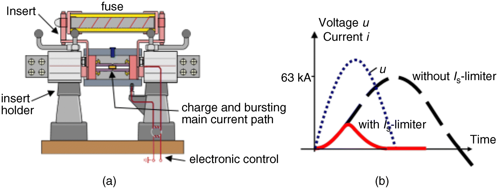
If the current is not allowed to be completely interrupted by the Is-limiter, a parallel combination of an Is-limiter with a reactor can be used. Upon tripping of the Is-limiter the current is commutated on the reactor, which limits the fault current. The elimination of the permanent resistive copper losses of the reactor makes the Is-limiter very cost-effective.
4.6 Conclusions
Effective protection is fundamental for the successful deployment of microgrids. The main challenges are posed by the interconnected DERs resulting in varying operating conditions depending on their status, reduced fault contribution by those interfaced by power electronic inverters and occasionally increased fault levels. This chapter focuses on automatic adaptive protection, in order to modify protection settings according to the microgrid configuration. Techniques to increase the amount of fault current level helped by a dedicated device, and possible use of fault current limitation are also discussed.
Appendices:
4.A.1 A Centralized Adaptive Protection System for an MV/LV Microgrid
In this Appendix a more elaborate application of the adaptive protection system based on pre-calculated settings is provided.
In the microgrid of Figure 4.31 the islanded operation is supported at two voltage levels: the complete MV microgrid can be disconnected from the utility grid and alternatively the LV microgrid can be disconnected from the MV microgrid.
Figure 4.31 A centralized adaptive protection system for the multilevel microgrid
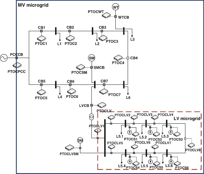
At the MV level, the system includes a single point of common coupling to the utility grid and a number of CBs controlled by IEDs equipped with a directional over-current protection function, shown in Figure 4.31 as PTOC. Each IED supports up to six independent setting groups and is fully compliant with IEC-61850 standard. All IEDs installed at the MV level are integrated into the centralized IEC-61850 automation system with a rugged controller installed at the primary substation (point of common coupling) serving as the core for making the control decisions, as well as providing data and event logging, reporting and human–machine interface (HMI) functionality.
At the LV level, the system consists of a number of LV circuit breakers also equipped with electronic trip units which are capable of performing directional over-current protection functions, and also support two setting groups and Modbus communications via a serial bus [11]. A centralized controller remote terminal unit (RTU) is installed at the point of coupling of the LV to MV networks at the secondary distribution substation. It provides both Modbus master and Modbus to IEC-61850 protocol conversion/gateway functionality, so that the data from the LV side may also be integrated into the centralized IEC-61850 automation system and considered in the programmed logic running at the MV primary station computer.
The controllers at both MV and LV levels communicate with the field protection devices at the corresponding levels and between each other. The main objective of the controllers is to adjust protection settings of each field relay with regard to the current state of the microgrid (both grid configuration and status of DERs are taken into consideration). It is effectuated by a programmed logic control continuously running in each controller for a periodic check and management of relay settings.
There are two major steps in the design and implementation of this concept:
- offline system configuration and
- online system operation.
4.A.1.1 Offline System Configuration
A set of the most common microgrid configurations and DER productions is created for offline fault analysis. Fault currents passing through all monitored CBs are calculated by simulating short circuits (3-phase, 2-phase, phase-to-ground etc.) at different locations of the protected microgrid. During repetitive short-circuit calculations a microgrid topology or the status of a single DER is modified between iterations.
Based on the simulation results, the settings for various network configurations are modeled for relevant microgrid configurations (e.g. islanded, grid-connected with DER off, grid-connected with DER on or radial/closed loop), and the IED setting groups are programmed accordingly.
For the MV part of the system (Figure 4.31), the various network configurations and topology changes that require control action – particularly changing the setting groups – are identified by the status of the corresponding circuit breakers in Table 4.7.
Table 4.7 Setting groups for network configurations at MV level
| CB status | Operating mode description | Corresponding setting group |
| PCCCB – on, SMCB, CB4 – off | Grid connected mode; radial; no large DG | SG1 |
| PCCCB – on, SMCB – on, CB4 – off | Grid connected mode; radial; Large DG contribution | SG2 |
| PCCB – off, SMCB. WTCB – on | Islanded | SG3 |
| All CBs on | Grid connected mode; closed loop; large DER contribution | SG4 |
If a breaker is not listed in the table, its status is unimportant for the control logic. Also, for convenience and to simplify the monitoring from the SCADA operator side, it is decided that all IEDs must adjust their setting groups to exactly the same active setting group number, even though in some cases the actual settings may be identical for several (all) setting groups. This is done so that situations are avoided where some of the IEDs, for example, are switched to setting group 2, while the others are still at setting group 1.
Electronic protection devices used at the LV level are only capable of keeping in memory two sets of setting groups. Therefore, we use the first setting group for the grid-connected mode and the second group is activated during islanded operation. However, we anticipate that future LV protection devices will have more than two setting groups which may further improve sensitivity, selectivity and speed of protection, especially during islanded operation of the microgrid with different types and sizes of DERs.
The next step after selection of setting groups is configuration of communications:
- IEC61850 for MV and
- Modbus-RTU for LV.
4.A.1.2 IEC 61850 Configuration
The overall offline engineering process for the proposed adaptive protection system is shown in Figure 4.32.
Figure 4.32 System configuration for a dynamic protection settings management at MV level
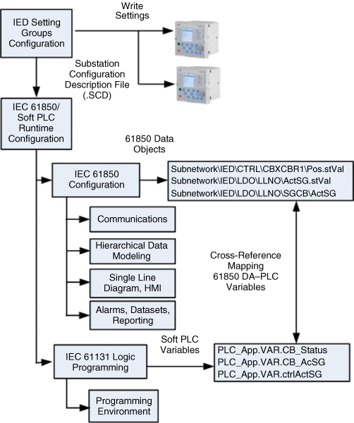
First, a system study is required to determine the IED settings for four setting groups in configurations outlined in Table 4.7, and the IEDs are configured remotely or via a local HMI.
Then the IEC 61850 automation system is created and the reporting is organized as follows. IEC 61850-7-4 Edition 2 defines the standard logical nodes and data objects related to the IED setting groups and circuit breaker position. IEC 61850-7-2 Edition 2 describes the mechanism and the associated abstract communication service interface (ACSI) for both reporting and control of the IED setting groups, which is called the setting group control block (SGCB). The ActSG service parameter of the setting group control block ACSI model can be used to read and write the new setting group value if a change is required due to certain changes in the microgrid topology.
Another standard data attribute used for monitoring the network configuration changes in the system is the circuit breaker position. It is a part of XCBR logical node and can also be included in a dataset. In terms of the IEC 61850 common data classes' definition, the circuit breaker position is described as controllable double point (DPC) with the status value data attribute stVal, which can take four values representing the four different possible states of the circuit breaker: 0 – intermediate, 1 – off, 2 – on, 3 – bad.
The ability to use the standard attributes is an important advantage of IEC 61850; it increases interoperability and allows for easy integration of the IEDs from multiple vendors into the automation system, although true plug-and-play functionality is not yet achieved. For instance, even though the circuit breaker position data attribute is standardized, it may be located in different logical devices for IEDs coming from different vendors.
For the purpose of changing the setting groups based on changes of microgrid topology, the status of the active setting group and the current circuit breaker position must be reported by the IEDs to the substation computer which runs the logic and takes the control decisions. In this case, the central controller (substation computer) acts as a client in the IEC 61850 client/server environment. Therefore these data objects must be either included in a dataset to which the substation computer will subscribe, or be configured to be sent as a GOOSE message. It has been found that the standard IEC 61850 dataset event reporting of the circuit breakers position provides acceptable performance. This method also saves bandwidth and simplifies sending the data across hybrid networks.
The substation computer is represented in the IEC 61850 SCL hierarchy as an IED client device with just one logical node for the HMI. Then the buffered report control blocks are configured for all actual IEDs to send the reports to the substation computer client spontaneously, that is, when a change of the circuit breaker position occurs.
To provide additional dependability, integrity reports may also be enabled, and the integrity polls issued by the client to retrieve and confirm the status of the circuit breaker periodically rather than spontaneously. If the integrity polls are used, it is recommended to create a separate dataset just for the active setting group and circuit breaker status to reduce bandwidth consumption, since the integrity poll will build a report containing all values of the referenced dataset, not just the ones that have been changed since the last poll.
The IEC 61850 data objects and attributes used to monitor the position of the circuit breaker and the active setting group status and control are summarized in Table 4.8.
Table 4.8 IEC 61850 standard data objects

4.A.1.3 Logic Processor Configuration
The logic processor is the brain of the adaptive protection system. It uses the IEC 61131-3 compatible languages to implement the logic used to extract the information received from the IEC 61850 communications infrastructure, perform the analysis and, if necessary, execute the control action by sending a control command back to the IEC 61850 automation system.
Table 4.9 illustrates the cross-mapping of the IEC 61850 objects to the PLC server variables for one of the IEDs.
Table 4.9 IEC 61850 to logic processor cross references
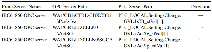
The rest of the IEDs are mapped in a similar manner, and the PLC variables are organized as arrays. The cross-reference mapping includes the direction which defines whether an IEC 61850 attribute is being monitored or controlled by the logic processor.
4.A.1.4 Communications Integration
The system includes the IEC 61850 OPC server, which integrates all the IEC 61850 compatible IEDs with the associated data objects. It also includes the logic processor OPC server which is responsible for monitoring and control. Additionally, the system contains an instance of Modbus TCP OPC server for the integration of the LV part of the network shown in Figure 4.31 through a TCP connection with LV RTU, as well as the DNP LAN slave OPC client used to map the data from the IEC 61850/Modbus microgrid automation system to the upstream DNP3 SCADA master.
4.A.1.5 Online Data Exchange and System Operation
The schematic diagram for the online operation of the system is shown in Figure 4.33.
Figure 4.33 Real-time communications architecture
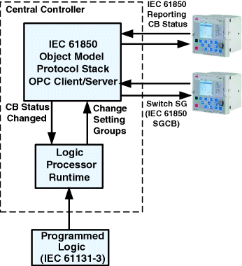
The real-time data exchange is organized as follows. The IEDs at the MV level use IEC 61850 communications; the substation computer runs the IEC 61850 OPC server, in order to receive the report data from the relays. It also executes the monitoring and control logic executed within the runtime logic processor engine. The IEC 61850 data attributes are mapped to the logic processor variables at the offline configuration stage as described in the previous section. Therefore, the logic processor application has fast access to the data received from the IEC 61850 side through the OPC data access mechanism and can detect the system events that will trigger the execution of the adaptive protection module and dictate the need for the control action. It must be noted that there is a delay associated with transferring the data between process signals and logic variables. The shortest possible data transfer cycle is 50 ms.
In situations where a setting's change is required, the logic processor runtime again uses the OPC DA mechanism to connect to the IEC 61850 environment and execute the command to change setting groups. The setting group change will only occur when the circuit breaker is in either on or off position; it will be inhibited if the status of the circuit breaker is undetermined (bad) or intermediate, which means that a circuit breaker is possibly in the middle of the reclosing sequence. The settings change will also be inhibited if the quality attribute of the IEC 61850 data object is bad. After the command to adjust the setting groups has been sent to the IEDs in the next cycle of its operation, the logic will read the ActSG status to make sure that the command was indeed successful.
The system also includes an additional OPC server instance, which can be used to map the microgrid communications data to the distribution network control center via SCADA. A protocol conversion may be executed at this step, if necessary; for example, IEC 61850 objects may be mapped to DNP3.
The logic developed with the IEC 61131-3 compatible tools can be used without changes at both MV and LV.
4.A.2 Description of the Prototype FCS
The circuit diagram of the prototype FCS is shown in Figure 4.34.
Figure 4.34 Circuit diagram of the prototype FCS
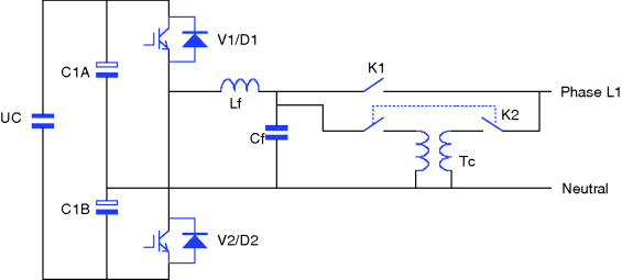
The ultra-capacitor stack UC is composed of 320 cells of 140 F connected in series. The cells are mounted on printed circuit boards each containing 16 cells plus voltage balancing resistors. Capacitors C1A and C1B are electrolytic capacitors acting as a DC-link capacitor in parallel to the IGBT stack. Electrolytic capacitors have a much lower ESR than the ultra-capacitor stack, and serve to reduce the ripple on the DC voltage during operation of the IGBTs. Also, the series connection of two capacitors is used to create a neutral connection to the network. The IGBT stack is formed by IGBTs V1 and V2 and by freewheeling diodes D1 and D2 in a half-bridge configuration. Both during charging and when operating during a fault, the half-bridge generates a pulse width modulated (PWM) sinusoidal voltage. The modulation frequency is 6 kHz. Inductor Lf and capacitor Cf together form the output filter of the FCS. The output filter removes the high-frequency components from the voltage generated by the half-bridge and converts the PWM voltage into a sinusoidal voltage. Moreover, inductor Lf acts as the output impedance of the FCS. The value of Lf is 3 mH, resulting in a physical output impedance of ∼1 Ω at 50 Hz.
Transformer Tc and contactors K2 form the pre-charging circuit of the FCS. If the ultra-capacitor stack is fully discharged, contactors K2 will be closed to start the charging sequence. The secondary no-load voltage of transformer Tc is 80 V. The impedance of the transformer and the inductor Lf together limit the rms AC input current to 50 A. The primary input current of the transformer is then 18 A, which is an acceptable load for the network. The voltage Uc across the ultra-capacitor increases to 150 VDC within 4 seconds. As soon as Uc > 150 VDC, the half-bridge starts switching. The PWM generation is controlled in such a way that the current in inductor Lf has an rms value of 10 A and that the current is in phase with the network voltage. Thus the reactive component is zero. In this way, the FCS takes a constant charging power of 800 W from the network. Subtracting the losses in transformer, inductor and IGBTs, the power delivered to the ultra-capacitor stack is ∼500 W. This part of the charging phase ends as soon as Uc > 600 VDC, which takes ∼2.5 minutes in this configuration. This DC voltage is high enough to justify direct connection of the half-bridge to the network. Consequently, contactors K2 are opened, and contactor K1 is closed. The control parameters of the PWM generation are changed to represent the new topology. Now the current in inductor Lf is controlled to an rms value of 4 A. The ultra-capacitor is further charged until Uc = 840 VDC (during the tests reported here, this maximum was set to 820 VDC).
For safety reasons the FCS may be required to store enough energy to clear more than one fault, because another fault could occur during the recharging period. On the other hand, the full energy content is only needed to trigger the biggest fuse on the most remote fault. If the clearing time is shorter than worst-case, only a small fraction of the energy content is absorbed during a single fault.
The control system operates according to the state transition diagram of Figure 4.35. The system has five operating states and two administrative states, which are described below. If the system was restarted or rebooted while there was still voltage in the DC buffer, the system would automatically proceed through the diagram until it reached the state which is most appropriate for the actual DC voltage. During a reboot, all contactors are opened and the IGBTs are switched to a passive state so that possibly destructive transients cannot occur.
- state 0 – Whenever a hardware-related fault has occurred, the system enters state 0. The system will remain in state 0 until all fault conditions have been removed and an appropriate delay time has elapsed. Within state 0, the fault reset logic has its own state machine.
- state 1 – When the FCS is started or the software is rebooted, the system enters state 1. In state 1, all variables are initialized. The FCS can be enabled/disabled from the user interface.
- state 2 – Contactors K2 are closed so that the ultra-capacitor is charged via the pre-charging transformer, and pre-charging continues until the DC voltage exceeds 2 to 3 times a threshold Uc, which is presently set to 150 VDC. When both the synchronization and the voltage threshold condition are fulfilled, the system will enter state 3.
- state 3 – Contactors K2 remain closed, but now PWM on the inverter will start so that the DC voltage can be further ramped up. The half-bridge is operated in current-control mode. The measured current in inductor Lf is decomposed into an active (in-phase) component and a reactive (out-of-phase) component. These components are the inputs of two controllers, whose outputs are used to calculate the phase and amplitude of the sinewave generated by the PWM. The reference for the reactive part is zero, the reference for the active part is set to −10 A. The minus sign is used because the positive polarity of the current is defined as flowing from the FCS into the grid. This state is finished when the DC voltage Uc is high enough for the inverter to be connected directly to the network, which is the case when Uc > 2*Ugrid, that is, twice the peak value of the grid voltage. The system then enters state 4.
- state 4 – This is the idle state, in which the system is ready for operation but remains idle, to minimize losses. Because both the ultra-capacitor stack and the electrolytic capacitors are provided with voltage sharing resistors, the DC voltage will decrease gradually and a regular top-up is needed to retain the voltage. This recharge is done in state 5 and is initiated if Uc < UCmin1. Threshold parameter UCmin1 is presently set to 780 V. This also means that if the system enters state 4 from state 3 (condition of transition: Uc > 2*Ugrid, which is in the order of 600 V), it will immediately move on to state 5. State 4 is purposely used as an intermediate state. A hardware interlock ensures that contactor K1 can only be closed after contactors K2 have opened and the system is only allowed to enter state 5 after the closing of contactor K1 has been confirmed.
- state 5 – The operation of state 5 is very similar to that of state 3. However, the inverter is now connected to the grid directly, instead of via the transformer, which means that the settings of the PWM are different and that the two current controllers use different control parameters and reference values. In state 5, the reactive current controller has a reference value of a few amps capacitive, so that the inverter will supply the capacitive current flowing into filter capacitor Cf. In this way, the power factor of the input current remains close to 1. In the prototype, the reference value for the active current controller is set to 4 A.
- state 6 – From both states 4 and 5, the system is allowed to enter state 6. This transition occurs when the fault detection logic has detected a probable fault in the network. During the transition to state 6, the sinewave generator for the PWM is detached from the phase-looked loop (PLL) and remains running with a fixed frequency value. The voltage dip associated with the fault may have caused the PLL to observe a frequency step. Therefore the measured value of the frequency is saved in a FIFO buffer in 100 ms. If a fault is detected, the PWM generation continues on the basis of a 100-ms-old value of the frequency, which generally will be a reliable pre-fault value. In state 6, the current controllers are inactive and the PWM uses a fixed amplitude for the output voltage, equal to the pre-fault value of Ugrid. In addition to that, the PWM calculation includes a virtual impedance which can virtually add both inductive and resistive components to the output inductor. With the lapse of time, the virtual impedance will increase, which makes it possible for the other generators in the network to regain control of the voltage and phase of the network. After a preset time – now set to 5 seconds – the FCS will leave state 6 and enter state 2. Depending on the remaining DC voltage after this action, the system may subsequently proceed to state 3, 4 or 5. If during its action in state 6, the DC voltage drops too low, defined as UC < Ucmin0, the system will immediately enter state 2. The value of Ucmin0 is presently set to 600 V.
Figure 4.35 State transition diagram of the FCS control system
1. Feero, W., Dawson, D., and Stevens, J. “Protection Issues of the Microgrid Concept”. Available http://certs.lbl.gov/pdf/protection-mg.pdf.
2. Al-Nasseri, H., Redfern, M.A., and O'Gorman, R. (2005) “Protecting microgrid systems containing solid-state converter generation”, Int. Conf. on Future Power Systems.
3. Vilathgamuwa, D.M., Loh, P.C., and Li, Y. (2006) Protection of microgrids during utility voltage sags. IEEE T. Ind. Electron., 53 (5), 1427–1436.
4. Driesen, J., Vermeyen, P., and Belmans, R. (2007) Protection issues in microgrids with multiple distributed generation units, 4th Power Conversion Conf., Nagoya.
5. Nukkhajoei, H. and Lasseter, R.H. (2007) “Microgrid Protection”, IEEE PES General Meeting.
6. EPRI (2006) “Overview of SEMI F47-0706” [online]. Available www.f47testing.com.
7. KEMA Limited (2005) “The contribution to distribution network fault levels from the connection of distributed generation”.
8. Bower, W. and Ropp, M. (March 2002) “Evaluation of islanding detection methods for photovoltaic utility interactive power systems,” IEA-PVPS, Online report T5-09. Available: http://www.oja-services.nl/iea-pvps/products/download/rep5_09.pdf.
9. Jayawarna, N. (2004) “Fault current contribution from power converters”, EU Microgrids project, Available www.microgrids.eu.
10. Rockefeller, G.D.et al. (1988) Adaptive Transmission Relaying Concepts for Improved Performance. IEEE Transactions on Power Delivery, 3 (4), 1446–1458.
11. ABB SACE SpA (2007), “Low voltage moulded case circuit breakers Tmax”, Product brochure, Available http://library.abb.com/global/scot/scot209.nsf/veritydisplay/117ea5b751d87f12c125734e002a25dc/$File/1SDC210015B0203.pdf.
12. ABB SACE SpA (2008), “DOC simulation tool”, User Manual version 1.0.
13. Shustov, A. and Valov, B. (2006) Lösungswege der Integrationsprobleme dezentraler Energieerzeugungsanlagen in elektrischen Verteilungsnetzen, Vorträge des internationalen wissenschaftlich-technischen Seminars, Polytechnische Universität Tomsk, 10.11.04.
14. CIGRE WG (2003) A3.10 “Fault Current Limiters – Fault Current Limiters in Electrical Medium and High Voltage Systems”, CIGRE Technical Brochure, No. 239.
15. CIGRE WG (2006) A3.16 “Guideline on the impacts of fault current limiting devices on protection systems”, A3-06 (SC) 33 IWD.
16. Lindmayer, M., Marzahn, E., Mutzke, A.et al. (2004) “The process of arc-splitting between metal plates in low voltage arc chutes”, 22nd Int. Conf. on Electrical Contacts, Seattle.
17. ABB Carol Emag (2008) “Is limiter”, Product brochure, Available http://library.abb.com/global/scot/scot235.nsf/veritydisplay/31656b3a0912262ac12574f700565d1e/$File/2243-08%20E_300dpi.pdf.