
Disks are the heart and soul of a database system—they physically store the data accessed by the database server. From both performance and high availability standpoints, ensuring a proper disk configuration is one of, if not the most, important aspect of planning and configuration when it comes to the system that will run Microsoft SQL Server 2000. Even though the decisions of how many processors and how much memory you need are important, you will probably get the most from your SQL Server investment by planning and implementing the best disk subsystem for your needs.
Whenever you design a system for availability, growth, and performance, as noted in Chapter 1, there is some form of tradeoff involved. This chapter guides you step by step through the decision-making, planning, and implementation of disk subsystems used with SQL Server.
This section defines a few terms that are used throughout the rest of the chapter.
Spindle. The physical disk itself. The term is derived from the shape of the disk inside the enclosure, which is a round platter with a head, somewhat resembling a spindle.
Logical Unit, LUN. This will be hardware and software vendor–dependent, but each of these terms has the same meaning—it is one physical disk or a group of disks that appear as one unit to the operating system at a physical level.
Important
If you want to configure more than eight LUNs, you must involve the hardware vendor in the planning and configuration. Microsoft Windows server products support up to eight buses per adapter, 128 target IDs per bus, and 254 LUNs per target ID. Adding support for more LUNs involves modifying the registry. See Chapter 5, for more information. Also keep in mind that your registry cannot grow infinitely large.
Logical Disk. A logical disk is part, or all, of a volume carved out and formatted for use with Windows, and is usually represented by a drive letter. Some storage vendors use the word containers, which can contain multiple logical volumes that represent one logical disk to Windows. In storage vendor language, this might be referred to as a LUN, which is not how LUN is defined here.
Numerous factors go into deciding how your disks will be configured. The first part of that decision process must be capacity planning, the art of determining exactly how much space you need. For new systems, this can range from very simple to very complex, depending on how much information you have up front. For extending existing systems, upgrading, or migrating to a new hardware or software platform, capacity planning should be easier because there should be documented history on the prior growth of that system, database, and application.
Two kinds of disk space usage must be known: raw space, and the physical number of disk drives needed for storage and to achieve the desired level of performance. Remember that figuring out how much raw space, which will then dictate how many drives you need, is based on your application’s requirements of how it will be using SQL Server. The information and equations are based on these basic tenets of disk capacity planning.
Note
The disk space presented by the disk controller at the LUN level and the disk space that is available to the application are not the same. All capacity planning must be based on the actual usable capacity as seen by Windows at the file system level, not what the storage controller thinks is being presented.
Important
Remember that any physical implementation is vendorspecific because each storage vendor might use similar—but different—architectures and structures.
Conceptually, the amount of raw disk space is represented by the following equation:
Minimum Disk Space Needed = Size of Data (per database, including system databases) + Size of All Indexes (per database, including system databases)
There is a flaw in this equation, however. Calculating your disk space based on the minimum amount needed would be a mistake. You need to take into account the growth of the database over the time that the system will be in service. That would transform the equation into this:
Minimum Disk Space Needed = Size of Data (per database, including system databases) + Size of All Indexes (per database, including system databases, full-text indexes, and so on) + Planned Growth + Microsoft Distributed Transaction Coordinator (MS DTC) Logging Space + Amount of Operating Reserve + Amount Reserved for Hardware Optimization
The revised equation is much more realistic. The amount of operating reserve is the total drive space needed to handle an emergency situation.
For example, if you need to add a new column to a table, you need enough transaction log space for the entire table (possibly two times the table) because all changes are logged row by row and the table is affected in its entirety within one transaction. The amount reserved for hardware optimization is based on the disk drive performance of the inner tracks of the physical drive, which might be slower than the outer tracks (see the section "Understanding Your Hardware" later in this chapter for information on media banding and physical drive characteristics).
In this case, the amount can range from 10 to 40 percent depending on whom you ask, but the performance characteristics might be different on more modern disk drives (up to 25 percent faster on the outer tracks than the inner tracks). You can combine this reserve space with the operating system reserve in most cases. With MS DTC usage, if you have high transactional volume, the logging of MS DTC might become a bottleneck.
Each application using SQL Server has its own signature that is its distinct usage of SQL Server. Assess each application that will be utilizing one or more databases. What kind of work is it doing? Is it mainly reads? Mainly writes? A mixture? Only reads? Only writes? If the workload is a combination of reads and writes, what is the ratio of reads to writes? (Some hardware solutions can assist you in this matter to report on real read versus write statistics, as well as storage caching statistics.) If this is an existing database system, how has the usage changed over time? If this is a new system, what is the projected usage of the system? Do you anticipate changes in usage patterns? You might need to ask more questions. For a packaged application that you are not developing, ensure that your vendor can reasonably answer the questions so you can plan your hardware appropriately. If possible, get the input of other customers who have used that software as well.
For example, an accounting package might have heavy inserts, for 70 percent on average, and 30 percent reads. Because the software is doing some aggregations at the SQL Server level and bringing back intermediate result sets, it also uses tempdb heavily. The company that manufactures the accounting package recommends a minimum of 60 GB as a starting size for the database, but you can best determine how the software would be used in your environment.
These questions are vital to starting the disk configuration process because, like the guiding principles that will carry through the entire high availability process, how the database is to be used directly influences every decision made about disk configuration.
Knowing the schema and how data is used also helps you determine the capacity needed. Important things to track are whether it is a custom in-house application or a third-party application; usage of data that is inserted, updated, and deleted; the most frequently used tables (for reads and writes); and how much these tables grow. A database administrator (DBA) or someone else, if appropriate, should track these items on a regular basis. Tracking these items over time for new and existing systems not only provides an accurate picture of your database usage, but also helps in areas such as performance tuning (figuring out what indexes to use, avoiding hotspotting at a physical level when designing a disk subsystem). If you have been using a database for years and now need to migrate it to a new version of the database software (for example, from Microsoft SQL Server 7.0 to Microsoft SQL Server 2000), you can accurately know how to configure your disk subsystem and SQL Server file sizes only if you know the answers to the above questions.
One consideration when thinking about schemas is the use or nonuse of Unicode. Unicode data is stored as nchar, nvarchar, and ntext data types in SQL Server as opposed to char, varchar and textr. This means that Unicode data types take up twice as much storage as non-Unicode data types, effectively halving how data is actually stored at a physical level (or doubling your space requirement, depending on how you look at it). This must be taken into account when calculating how much each row will total in terms of bytes—if a row that is non-Unicode is 8000 bytes, for a Unicode row it will be 16,000 bytes.
Another consideration is fixed-length versus variable-length text columns. To be able to predict row length, and ultimately table growth over time, you should use fixed-length fields such as a char instead of a varchar. A varchar also consumes more disk space. If you are writing an application that must support international customers in different languages, you need to account for the space required for each language. Therefore, if you are writing an application that must store information in English, French, Spanish, Dutch, Japanese, and German, you need to account for up to six different versions of each column. As with many other things related to system and application designs, there are trade-offs when it comes to schema design.
For example, you have an application that accesses a table named CustomerInfo. Table 4-1 shows the table structure.
Table 4-1. CustomerInfo Table
Column Name | Type/Length | Column Size (in Bytes) |
|---|---|---|
Customer_id | Int | 8 |
Customer_lname | char(50) | 50 |
Customer_fname | char(50) | 50 |
Cust_addr1 | char(75) | 75 |
Cust_addr2 | char(75) | 75 |
Cust_city | char(30) | 30 |
Cust_state | Int | 8 |
Cust_province | char(40) | 40 |
Cust_postalcode | char(15) | 15 |
Cust_country | Int | 8 |
Total | 359 |
According to Table 4-1, each row inserted into the CustomerInfo table consumes 359 bytes. Assume that this is an e-commerce application, and the database is expected to grow to 500,000 customers in two years. That equates to 179,500 kilobytes, or just fewer than 180 MB for this table alone. Each entry might also include updates to child tables (such as customer profiles or customer orders). With each insert, you need to take into account all parts of the transaction. If your table has 10, 20, 50, 100, or 500 tables in it, suddenly 180 MB is only a small part of the puzzle. If you have not gathered already, things get complex very quickly when it comes to disk architecture.
Important
Remember to take into account columns that might also be able to contain a value of NULL, such as VARCHAR. Most column types require the same space at a physical level even if you use NULL and technically do not store data. This means that if you do not count the nullable column into your row size calculations in determining how many rows fit per page, you might cause page splits when actual data is inserted into the row.
Indexes are integral to a schema and help queries return data faster. Take performance out of the equation for a moment: each index takes up physical space. The total sum of all indexes on a table might actually exceed or equal the size of the data. In many cases, it is smaller than the total amount of data in the table.
There are two types of indexes: clustered and nonclustered. A clustered index is one in which all the data pages are written in order, according to the values in the indexed columns. You are allowed one clustered index per table. Clustered indexes are great, but over time, due to inserts, updates, and deletions, they can become fragmented and negatively impact performance.
Indexes can help or hurt performance. UPDATE statements with corresponding WHERE clauses and the right index can speed things up immensely. However, if you are doing an update with no WHERE clause and you have several indexes, each index containing the column being updated needs to be updated.
In a similar vein, if you are inserting a row into a table, each index that contains the row has to be updated, in addition to the data actually being inserted into the table. That is a lot of disk input/output (I/O). Then there is the issue of inserting bulk data and indexes—indexes hinder any kind of bulk operation. Think about it logically—when you do one insert, you are not only updating the data page, but all indexes. Multiply that by the number of rows you are inserting, and that is a heavy I/O impact no matter how fast or optimized your disk subsystem is at the hardware level. For performing bulk inserts, indexes should be dropped and re-created after the inserting of the data in most cases.
Queries might or might not need an index. For example, if you have a lookup table with two columns, one an integer, and one a fixed length of five characters, putting indexes on the table, which might only have 100 rows, could be overkill. Not only would it take up more physical space than is necessary, but also a table scan on such a small amount of data and rows is perfectly acceptable in most cases.
More Info
You also need to consider the effect of automatic statistics and their impact on indexes. See the sections "Index Statistics" and "Index Cost" in Chapter 15 of Inside Microsoft SQL Server 2000 by Kalen Delaney (Microsoft Press, 2000, 0-7356-0998-5) for more information. SQL Server Books Online (part of SQL Server documentation) also explores indexes in much more detail than what is offered here.
The code you write to delete, insert, select, and update your data is the last part of the application troika, as it contains the instructions that tell SQL Server what to do with the data. Each delete, insert, and update is a transaction. Optimizing to reduce disk I/O is not an easy task because what is written is directly related to how well designed the schema is and the indexing scheme used. The key is to return or update only the data that you need, keeping the resulting transaction as atomic as possible. Atomic transactions and queries are ones that are kept extremely short. (It is possible to write a poor transaction that is seemingly atomic, so do not be misled.) Atomicity has an impact on disk I/O, and in terms of technologies like log shipping and transactional replication, the smaller the transaction that SQL Server has to handle, the better off you are in terms of availability.
For example, a Web-based customer relationship management (CRM) program used by your sales force allows you to access your company’s entire customer list and page through the entries one by one. The screen only displays 25, and at a maximum, displays up to 200. Assume the schema listed earlier for the CustomerInfo table is used. The application developer implements this functionality by issuing a SELECT * FROM CustomerInfo query with no WHERE clause; as you might have deduced, the combination of a SELECT * that pulls back all columns and no WHERE clause to narrow the result set is not recommended. The application then takes the results and displays only the top 200 customers. Here is the problem with this query: when you reach 500,000 customers, every time this functionality is called, it returns 180 MB of data to the client. If you have 500 salespeople, 100 of whom are always accessing the system at one time, that is 18,000 MB or 18 GB of data that can potentially be queried at the same time. Not only will you be thrashing your disks, but network performance will also suffer. A better optimization would be to issue the same query with a TOP 200 added so that you are only returning the maximum result set handled by the application. Another way to handle the situation is to make the rowcount a parameter allowing each user to customize how many rows he or she would like returned, but that would not guarantee predictability in the application.
To make matters worse, if the user wanted to do different sorts, the application developer would not utilize the 180 MB result set that was already queried: he or she issues another SELECT * FROM CustomerInfo query, this time with a sorting clause (such as ORDER BY Customer_lname ASC). Each round trip, you are thrashing disks and consuming network bandwidth when you want to do a sort! If there were any sort of action associated with the rows returned, you would now have multiple users going through the list in different directions, potentially causing deadlocks and compounding the problem. Unless the data that will be pulled back changes, the application should be able to handle the sort of the data for display without another round trip. If you need to pull back different data, using a WHERE clause combined with the aforementioned TOP also helps disk I/O, especially if you have the proper indexing scheme, as you can go directly to the data you are looking for.
Transact-SQL statements that use the locking hints in SQL Server, such as HOLDLOCK, NOLOCK, and so on can either help or hinder SQL Server performance and availability. You should not use locking hints because the query processor of SQL Server in most cases chooses the right locking scheme behind the scenes as its default behavior. For example, a user of the same CRM application updates a row into the CustomerInfo table. The developer, with the best of intentions, wants to ensure that no one else can update the record at the same time, so naively he or she adds the XLOCK hint to the UPDATE statement. Adding XLOCK forces the transaction to have an exclusive lock on the Customer-Info table. This means that no other SELECT, INSERT, UPDATE, or DELETE statements can access the table, backing up requests for SQL Server, backing up disk resources, and causing a perceived unavailability problem in the application because the users cannot do their work. Thus one seemingly small decision can affect not only many people, but also various resources on the server.
If you are using a database now, or are testing one that is going into production, you need to capture statistics about what is going on at the physical and logical layers from a performance perspective under no load, light load, medium load, and heavy load scenarios. You might be set with raw disk capacity in terms of storage space, but do you already have a performance bottleneck that might only get worse on a new system configured in the same way?
For Microsoft Windows 2000 Server and Microsoft Windows Server 2003, disk performance counters are permanently enabled. If, for some reason, they are not currently configured in Performance Monitor (they should appear as the LogicalDisk and PhysicalDisk categories), execute DISKPERF –Y to enable the disk performance counters at the next system restart. Obviously, this causes a potential availability problem if a restart is required immediately. For more information about the different options with DISKPERF, execute DISKPERF /? at a command prompt. Having the disk performance counters turned on adds approximately 10 percent of overhead to your system.
Once the disk performance counters are enabled, you can begin capturing information to profile your disk usage. There are two types of disk statistics to consider:
The most important statistics are the physical counters, although the logical ones could help in some environments. It really depends on how your disk subsystem is configured and what is using each physical and logical disk. More on logical and physical disks is covered in the section "Pre-Windows Disk Configuration" later in this chapter.
The performance counters described in Table 4-2 should provide you with a wealth of information about your disk subsystem.
Table 4-2. Performance Counters
Category | Counter | Purpose | How to Interpret |
|---|---|---|---|
Physical Disk | % Disk Time—track for each physical disk used | Percentage of the elapsed time that the selected physical disk drive has spent servicing read and write requests. | This number should be less than 100 percent. However, if you are seeing sustained high utilization of the physical disk, it might either be close to being overutilized, or should be tracked according to its mean time between failures (MTBF). For further follow-up or information, % Disk Read Time and % Disk Write Time can be tracked. |
Physical Disk | Avg. Disk Queue Length—track for each physical disk used | The average number of requests (both reads and writes) that were waiting for access to the disk during the sample interval. | Realistically, you want the number to be 0. However, 1 is acceptable, 2 could indicate a problem, and above 2 is definitely a problem. However, keep in mind that this is relative—there might not be a problem if the queuing is not sustained, but was captured in one interval (say, one reading of 3), or if it is sustained. Remember that the number should not be divided by the number of spindles that make up a LUN. Queuing relates to the single worker thread handling the physical volume and therefore still represents a bottleneck. Follow-up or additional information can be captured with Avg. Disk Read Queue Length, Avg. Disk Write Queue Length, and Current Disk Queue Length for more isolation. |
Physical Disk | Avg. Disk sec/Read | The average time (in seconds) it takes a read of data to occur from the disk. | This can be used to help detect latency problems on disk arrays, especially when combined with the total number of updates and the aggregate number of indexes. |
Physical Disk | Avg. Disk sec/Write | The average time (in seconds) it takes a write of data to occur from the disk. | This can be used to help detect latency problems on disk arrays, especially when combined with the total number of updates and the aggregate number of indexes. |
Physical Disk | Disk Bytes/sec—track for each physical disk used | The total amount of data (in bytes) at a sample point that both reads and writes are transferred to and from the disk. | This number should fit the throughput that you need. See "Pre-Windows Disk Configuration" for more details. For more information or follow-up, Disk Read Bytes/sec and Disk Write Bytes/sec can further isolate performance. The average, and not actual value, can also be tracked in addition to or instead of this counter (Avg. Disk Bytes/Read, Avg. Disk Bytes/Transfer, Avg. Disk Bytes/Write). |
Physical Disk | Disk Transfers/sec—track for each physical disk used | The sum of all read and write operations to the physical disk. | For more information or follow-up, Disk Reads/sec and Disk Writes/sec further isolate performance. |
Physical Disk | Avg. Disk sec/Transfer | The time (in seconds) on average it takes to service a read or write to the disk. | Sustained numbers mean that the disks might not be optimally configured. For follow-up or more isolation, use Avg. Disk sec/Read and Avg. Disk sec/Write. |
Physical Disk | Split IO/sec | The rate (in seconds) at which I/Os were split due to a large request or something of that nature. | This might indicate that the physical disk is fragmented and is currently not optimized. |
% Free Space—track for each logical disk used | The amount of free space available for use. | This should be an acceptable number for your organization. Note that with NTFS, there is something called the master file table (MFT). There is at least one entry in the MFT for each file on an NTFS volume, including the MFT itself. Utilities that defragment NTFS volumes generally cannot handle MFT entries, and because MFT fragmentation can affect performance, NTFS reserves space for MFT to keep it as contiguous as possible. With Windows 2000 and Windows Server 2003, use Disk Defragmenter to analyze the NTFS drive and view the report that details MFT usage. Remember to take MFT into your free space account. Also keep in mind that database disks rarely get extremely fragmented because file creation does not happen as often (unless you are expanding frequently or using the SQL disks for other purposes). | |
Logical Disk Free Megabytes | The amount of free space on the logical drive, measured in megabytes. | As with % Free Space, this should be at an acceptable level. | |
Some of the counters in Table 4-2, such as Avg. Disk sec/Transfer, have equivalents in the LogicalDisk category. It is a good idea to further isolate and gather performance statistics to track numbers for each logical disk used by SQL Server to help explain some of the numbers that occur on the PhysicalDisk counters.
SQL Server can also help you understand what is happening with your disk usage. SQL Server has a function named fn_virtualfilestats that provides I/O information about all of the files (data, log, index) that make up an individual database. fn_virtualfilestats requires the number of the database you are looking for statistics about, which can be gathered by the following query:
SELECT * FROM master..sysdatabases
Or you could use the following:
sp_helpdb
To see the actual names of the files used in your database, execute the following query:
SELECT * FROM databasename..sysfiles
Finally, to get the statistics for all files for a specified database, execute a query using fn_virtualfilestats. It takes two parameters: the database ID, which is the first number, and the file number. If you want to return all files, use -1 for the second parameter. This example retrieves the results for all files used with pubs, as shown in Figure 4-1.
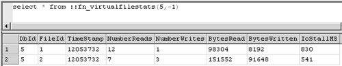
Figure 4-1. The results of a query designed to show the I/O statistics for all files comprising the pubs database.
If you take the data returned from the IOStallMS column and divide by the sum of NumberReads and NumberWrites (IOStallMS/[NumberReads+Number-Writes]), the result determines if you have a log bottleneck.
There are three main types of disk subsystems you need to understand when putting together a SQL Server solution: Direct-Attached Storage (DAS), Network-Attached Storage, and storage area networks (SANs).
Direct-Attached Storage (DAS) is the traditional SCSI bus architecture. There are quite a few variations of SCSI, and describing them all is beyond the scope of this chapter. With DAS, you have a disk or set of disks dedicated to one host, or in the case of a failover cluster, potentially available to the nodes. SCSI has some inherent cabling issues, such as distance limitations, and adding a new disk with DAS can cause an availability outage. One of the biggest problems with DAS is that when it is used with a server cluster, you have to turn all caching off, so you take a potential performance hit because the redundant array of independent disks (RAID) controllers are located in each node. However, this can vary with each individual hardware implementation. If the node’s SQL Server resources fail to the other node and there are uncommitted transactions in the cache of the local controller, assuming that node is not cycled and you fail the resources back at some point, you then potentially corrupt your data when the original node sees the disks again and flushes its cache.
Keep in mind that if the material in the cache is not something that needs to be written to the log (such as an insert, update, or delete), it might not matter. SQL Server automatically rolls back any unfinished transactions in a failover.
Network-Attached Storage devices are fairly new to the storage arena. These devices are function-focused file servers that enable administrators to deploy and manage a large amount of disk storage in a single device. Network-Attached Storage behaves like any other kind of server—it integrates into a standard IP-based network to communicate with other clients and servers. Some storage vendors present Network-Attached Storage as a DAS device. Network-Attached Storage is usually used for file-based storage, but it can be used with SQL Server if it meets all of your performance, availability, and other goals. Besides generic Network-Attached Storage devices, there are also Windows-powered Network-Attached Storage devices based on Windows 2000 that are optimized and preconfigured for file storage. Before purchasing a Network-Attached Storage–based SQL Server storage solution, consider the following:
If you do not use a Windows Hardware Quality Labs (WHQL) certified Network-Attached Storage, it might not meet the I/O guarantees for a transactional database, although it might work with your SQL Server solution. Should there be data corruption due to use of a non-WHQL certified Network-Attached Storage, Microsoft will not support the data-related issues and instead will refer you to the Network-Attached
Storage vendor for support. Check with your vendor about compatibility of the device for use with SQL Server and database systems. If the Network-Attached Storage device offers support for snapshot backup using split-mirror (with or without copy-on-write), the Network-Attached Storage device must support the SQL Server Virtual Device Interface (VDI) for backups. The vendor-supplied Network-Attached Storage utilities and third-party software should also support the VDI if this functionality is needed. If the VDI is not supported, availability could be impacted (SQL Server would need to be stopped so that the mirror could be split) or the SQL Server databases could become corrupt (by splitting the mirror without allowing SQL Server to cleanly flush pending writes and leaving the databases in a consistent state for backup).
Make sure that your network bandwidth can handle the traffic that will be generated by SQL Server to and from the Network-Attached Storage devices. Consider a dedicated network that will not impact any other network traffic.
SQL Server 2000 failover clustering is currently not a supported configuration with Network-Attached Storage as the disk subsystem. SQL Server 2000 currently only supports stand-alone instances for use with Network-Attached Storage.
For a normal non-Network-Attached Storage–based SQL Server installation, if the network or a network card malfunctions, it is probably not a catastrophic failure because SQL Server and its disk subsystem are properly working. On a clustered SQL Server installation, a network or a network card malfunction can result in a SQL Server restart and possible failover of the service. This implication does not apply because Network-Attached Storage use is not supported with virtual servers. Because Network-Attached Storage solutions are based on the network and network card being available, you must guarantee 100 percent uptime for the network and network card to avoid any data problems, data corruption, or data loss.
If you are using RAID, make sure that the Network-Attached Storage device supports the level of RAID that will give you the performance and availability that you require.
When deploying Network-Attached Storage for a transactional database, contact the Network-Attached Storage vendor to ensure that the device is properly configured and tuned for use with a database.
Prior to making any storage purchase decisions, you need to determine the required disk throughput, disk capacity, and necessary processor power. If you are considering a Network-Attached Storage solution, these additional requirements need to be taken into account:
Network-Attached Storage performance is dependent on the Internet Protocol (IP) stack, the network interface card, other networking components, and the network itself. If Network-Attached Storage is used as the data store for SQL Server, all database I/O is processed by the network stack instead of the disk subsystem (as it would be in DAS) and is limited by the network’s bandwidth.
Because processor utilization can increase with database load, only databases with a smaller load should be used with Network-Attached Storage. However, if a high-speed switched network interconnect is used between your SQL Server and Network-Attached Storage device, such as the Virtual Interface Architecture (VIA), processor utilization and network latency can be reduced for every SQL Server I/O. If you have a multiprocessor system, you need multiple network cards, and vice versa: if you have multiple network cards, you need multiple processors, otherwise you might see unbalanced processor loads, especially in a high-bandwidth network or Network-Attached Storage environment.
Most networks are configured at 10 or 100 megabits (Mb). This means that Network-Attached Storage performance might be significantly less than that of DAS or SANs, which are optimized for high disk transfer rates.
If many Network-Attached Storage devices are placed on a shared network, they might consume a large portion of network bandwidth. This has a significant impact not only on SQL Server, but also on anything else accessing the network.
SQL Server is not configured by default to support the creation and usage of a data store on a network file share, either those located on a standard server or a Network-Attached Storage device. In the case of Network-Attached Storage, data corruption could occur due to network interruptions if the process that ensures database consistency issues a write that cannot be committed to the disks of the Network-Attached Storage device.
To enable support for network file shares, trace flag 1807 must be enabled. This trace flag bypasses the check to see if the location for the use and creation of the database file is on a network share. Use Query Analyzer, select the master database, and execute the following command:
DBCC TRACEON(1807)
The successful result of this command should be as follows:
DBCC Execution Completed. If DBCC Printed Error Messages, Contact Your
System Administrator.
It is now possible to use a mapped drive or a Universal Naming Convention (UNC) path (that is, \servernamesharename) with SQL Server 2000. If trace flag 1807 is not enabled prior to using a Network-Attached Storage device with SQL Server, you will encounter one of the following errors:
5105 (Device Activation Error)
5110 (File ’file_name’ Is On A Network Device Not Supported For Database Files).
Warning
Although the preceding section illustrates how SQL Server can be configured to use Network-Attached Storage for its data store, remember that the usage is currently limited to a stand-alone SQL Server installation. A clustered SQL Server installation is not supported using Network-Attached Storage. Consult http://support.microsoft.com to see if this changes in the future.
SANs are a logical evolution of DAS, and they fix many of the issues, such as the caching problem, associated with DAS. The purpose of a SAN is to give you flexibility, scalability, availability, reliability, security, and device sharing. SANs cache work at the physical level on the disk of sectors, tracks, and cylinders.
SQL Server itself technically does not care what protocol you use to access your SAN, but your choice impacts performance. SCSI and Fibre Channel have been mentioned, but there is also the VIA protocol, traditional IP, Ethernet, and Gigabit Ethernet. Fibre Channel, which does have some low-level SCSI still embedded, is strongly recommended. It is the most effective at carrying blocktype data from storage to the computer writing or reading data. It also delivers predictable performance under higher loads than traditional Ethernet loads. Most important, Fibre Channel is extremely reliable.
More Info
Remember to separate the transport from the actual protocol. For example, iSCSI, Fibre Channel, and VIA are transports. Typically the block transfer protocol on top is SCSI. So, for example, iSCSI is SCSI over IP. Fibre Channel fabrics are SCSI over Fibre Channel, and so on.
The speed of your SAN is largely related to its architecture, which has a host bus adapter that is in each server accessing the SAN, controllers for the disk, switches, and finally, the disks themselves. Each manufacturer implements SANs a bit differently, although the overall concepts are the same, so it is important to work with your hardware vendor to ensure you understand what you are implementing.
From a security standpoint, with a SAN, you can do things like zoning and masking, although your SAN vendor must support these features. Zoning occurs when you set up the SAN so that systems can be isolated from one another, and this feature is very useful for clustering. Masking allows you to hide LUNs from certain systems. Cluster nodes can be in the same or different, overlapping zones that are configured with masking.
Because SANs support a wide range of operating systems and servers, a company might purchase a large SAN for use with many different servers or types of workload. Although it is good that you have a SAN, you need to realize the implications of this. Because all systems attached to the system have different workloads and the SAN only has one cache, you will be sharing the cache among multiple systems. If, for example, you also have an Exchange server on your SAN that is heavily utilizing the cache, this could impact the performance of your SQL Server.
Also consider how the other operating systems or applications interface with the SAN at a base level—if another Windows server or cluster issues a bus reset as it comes online (say, after a reboot of a node), will it affect your current Windows server or cluster with SQL Server that is running with no problems? These are things you should know prior to putting the SAN into production.
You might also be sharing spindles between different servers on a SAN depending on how the vendor implemented its disk technology. What this means is that one physical disk might be carved up into multiple chunks. For example, a 36-GB disk might be divided into four equal 9-GB partitions at a physical level that Windows and SQL Server would never even see; they only see the LUN. You must recognize if your hardware does this and plan accordingly.
With so many choices available to you, what should you choose? Simply put, choose what makes sense for your business from many standpoints: administration, management, performance, growth, cost, and so on. This is not like other decisions you will make for your high availability solution, but it might be one of the most important technology decisions you make with regard to SQL Server. When considering cost versus performance, features, and so on, look at the long-term investment of your hardware purchase. Spending $100,000 on a basic SAN might seem excessive when compared to a $10,000 traditional DAS solution, but if your company is making millions of dollars per month, and downtime will affect profitability, over time, that SAN investment gets cheaper. The initial cost outlay is usually a barrier, however.
As you might have gathered, Network-Attached Storage is currently not the best solution when you want to configure SQL Server. From an availability standpoint, your network is one large single point of failure, and the possibility of data corruption due to network interruption decreases your availability if you need to restore from a backup.
That leaves DAS and SAN. At this point the main issues will be cost, supportability, and ease of expansion and administration. DAS is usually SCSI-based and it is much cheaper, but it is less flexible, and because you cannot, for example, use the write cache (read is just fine), it might not be ideal for your high availability usage of SQL Server. SANs are the way to go if you can afford a solution that fits your needs. The ease of configuration and expansion as well as flexibility are key points to think about when looking at SANs.
Although they are not mentioned directly, there is always the option (in a nonclustered system) to use separate disks internal to a system, whether they are SCSI or Integrated Device Electronics (IDE). Some internal SCSI disks also support RAID, which is described in more detail in the section "A RAID Primer" later in this chapter.
There are two types of storage I/O technologies supported in server clusters: parallel SCSI and Fibre Channel. For both Windows 2000 and Windows Server 2003, support is provided for SCSI interconnects and Fibre Channel arbitrated loops for two nodes only.
Important
For larger cluster configurations (more than two nodes), you need to use a switched Fibre Channel (fabric/fiber-optic, not copper) environment.
If you are implementing SCSI, the following considerations must be taken into account:
It is only supported in Windows 2000 Advanced Server or Windows Server 2003 up to two-nodes.
SCSI adaptors and storage solutions need to be certified.
SCSI cards that are hosting the interconnect should have different SCSI IDs, normally 6 and 7. Ensure device access requirements are in line with SCSI IDs and priorities.
SCSI adaptor BIOS should be disabled.
If devices are daisy-chained, ensure that both ends of the shared bus are terminated.
Use physical terminating devices and do not use controller-based or device-based termination.
SCSI hubs are not supported.
Avoid the use of connector converters (for example, 68-pin to 50-pin).
Avoid combining multiple device types (single ended and differential, and so on).
If you are implementing Fibre Channel, the following considerations must be taken into account:
Fibre Channel Arbitrated Loops (FC-AL) support up to two nodes.
Fibre Channel Fabric (FC-SW) support all higher combinations.
Components and configuration need to be in the Microsoft Hardware Compatibility List (HCL).
You can use a multicluster environment.
Fault-tolerant drivers and components also need to be certified.
Virtualization engines need to be certified.
When you really think about it, clusters are networked storage configurations because of how clusters are set up. They are dependent on a shared storage-infrastructure. SCSI-based commands are embedded in fiber at a low level. For example, clustering uses device reservations and bus resets, which can potentially be disruptive on a SAN. Systems coming and going also lead to potential disruptions. This behavior might change with Windows Server 2003 and SANs, as the Cluster service issues a command to break a reservation and the port driver can do a targeted or device reset for disks on Fibre Channel (not SCSI). The targeted resets require that the host bus adapter (HBA) drivers provided by the vendor for the SAN support this feature. If a targeted reset fails, the traditional entire buswide SCSI reset is performed. Clusters identify the logical volumes through disk signatures (as well as partition offset and partition length), which is why using and maintaining disk signatures is crucial.
Clusters have a disk arbitration process (sometimes known as the challenge/defense protocol), or the process to reserve or "own" a disk. With Microsoft Windows NT 4.0 Enterprise Edition, the process was as follows: for a node to reserve a disk, it used the SCSI protocol RESERVE (issued to gain control of a device; lost if a buswide reset is issued), RELEASE (freed a SCSI device for another host bus adapter to use), and RESET (bus reset) commands. The server cluster uses the semaphore on the disk drive to represent the SCSI-level reservation status in software; SCSI-III persistent reservations are not used. The current owner reissues disk reservations and renews the lease every 3 seconds on the semaphore. All other nodes, or challengers, try to reserve the drive as well. Before Windows Server 2003, the underlying SCSI port did a bus reset, which affected all targets and LUNs. With the new StorPort driver stack of Windows Server 2003, instead of the behavior just described, a targeted LUN reset occurs. After that, a wait happens for approximately 7 to 15 seconds (3 seconds for renewal plus 2 seconds bus settle time, repeated three times to give the current owner a chance to renew). If the reservation is still clear, the former owner loses the lease and the challenger issues a RESERVE to acquire disk ownership and lease on the semaphore.
With Windows 2000 and Windows Server 2003, the arbitration process is a bit different. Arbitration is done by reading and writing hidden sectors on the shared cluster disk using a mutual exclusion algorithm by Leslie Lamport. Despite this change, the Windows NT 4.0 reserve and reset process formerly used for arbitration still occurs with Windows 2000 and Windows Server 2003. However, the process is now used only for protecting the disk against stray I/Os, not for arbitration.
More Info
For more information on Leslie Lamport, including some of his writings, go to http://research.microsoft.com/users/lamport/. The paper containing the fast mutual exclusion algorithm can be found at http://research.microsoft.com/users/lamport/pubs/pubs.html#fast-mutex.
As of Windows 2000 Service Pack 2 or later (including Windows Server 2003), Microsoft has a new multipath I/O (MPIO) driver stack against which vendors can code new drivers. The new driver stack enables targeted resets using device and LUN reset (that is, you do not have to reset the whole bus) so that things like failover are improved. Consult with your hardware vendor to see if their driver supports the new MPIO stack.
Warning
MPIO is not shipped as part of the operating system. It is a feature provided to vendors by Microsoft to customize their specific hardware and then use. That means that out of the box, Windows does not provide multipath support.
When using a SAN with a server cluster, make sure you take the following into consideration:
Ensure that the SAN configurations are in the Microsoft HCL (multicluster section).
When configuring your storage, the following must be implemented:
Zoning. Zoning allows users to sandbox the logical volumes to be used by a cluster. Any interactions between nodes and storage volumes are isolated to the zone, and other members of the SAN are not affected by the same. This feature can be implemented at the controller or switch level and it is important that users have this implemented before installing clustering. Zoning can be implemented in hardware or firmware on controllers or using software on hosts. For clusters, hardware-based zoning is recommended, as there can be a uniform implementation of access policy that cannot be disrupted or compromised by a node failure or a failure of the software component.
LUN masking. This feature allows users to express a specific relationship between a LUN and a host at the controller level. In theory, no other host should be able to see that LUN or manipulate it in any way. However, various implementations differ in functionality; as such, one cannot assume that LUN masking will always work. Therefore, it cannot be used instead of zoning. You can combine zoning and masking, however, to meet some specific configuration requirements. LUN masking can be done using hardware or software, and as with zoning, a hardware-based solution is recommended. If you use software-based masking, the software should be closely attached to storage. Software involved with the presentation of the storage to Windows needs to be certified. If you cannot guarantee the stability of the software, do not implement it.
Firmware and driver versions. Some vendors implement specific functionality in drivers and firmware and users should pay close attention to what firmware and driver combinations are compatible with the installation they are running. This is valid not only when building a SAN and attaching a host to it, but also over the entire life span of the system (hosts and SAN components). Pay careful attention to issues arising out of applying service packs or vendor-specific patches and upgrades.
Warning
If you are going to be attaching multiple clusters to a single SAN, the SAN must appear on the both the cluster and the multicluster lists of the HCL. The storage subsystem must be configured (down to the driver level, fabric, and HBA) as described on the HCL. Switches are the only component not currently certified by Microsoft. You should secure guarantees in writing from your storage vendor before implementing the switch fabric technologies.
Tip
Adding a disk to a cluster can cause some downtime, and that amount of downtime is directly related to how much you can prepare for it. If you have the disk space, create some spare, formatted LUNs available to the cluster if you need to use them. This is covered in more depth in Chapter 5.
Now that you understand how to calculate disk capacity from a SQL Server perspective, it is time to put that knowledge into planning and action. Disks require configuration before they can be presented to Windows and, ultimately, SQL Server. A few tasks must be performed prior to configuring a disk in Windows to allow SQL Server to use it.
How many disks do you need to get the performance you desire and the space you need? Calculate the number of spindles (actual disks) based on the application data you have gathered or should have available to you.
Important
Remember when figuring out the number of spindles needed to take into account how many will make up a LUN. Some hardware vendors allow storage to be expanded only by a certain number of drives at a time, so if you need to add one disk, you might actually need to add six. Also, just because your storage vendor supports a certain number of spindles per LUN, it does not mean you should actually use that many disks. Each vendor has its own optimal configuration, and you should work with the vendor to determine that configuration.
This is the easiest of the calculations. For this, you need to know the following:
The number of concurrent users
The amount of data each user is returning
The time interval used by the user
Assume you have 250 concurrent users. Each needs to simultaneously bring back 0.5 MB of data in less than one second. This means that in total, you must be able to support constantly bringing back 125 MB of data from your disk subsystem in less than a second, every second, to get the performance you desire.
It is time to calculate the throughput of a single physical drive. You must know the following information:
Maximum I/Os supported for the physical drive in its desired configuration (that is, RAID level, sector size, and stripe size are factors).
Ratio of 8k page reads to 64k readaheads for the operations. You might not know this information, but it is ultimately useful. You can use the numbers shown here as a rough estimate if you do not know. Each drive is rated at a certain number of I/Os that the hardware manufacturer should be able to provide.
Continuing from step 1, assuming 80 percent 8k page reads and 20 percent 64k readaheads, and knowing that the drive can support 100 I/Os per second:
Note
Individual drive throughput might or might not be as important with SANs as it is with DAS. It depends. Because high-end storage subsystems might have lots of cache space, physical performance can be optimized, compensated for, or masked by the architecture of the solution. This does not mean you should buy lower speed 5400 rpm speed disks. It just means you should understand the physical characteristics of your disk subsystem.
Now that you have the amount of data being returned and the throughput of the individual drive, you can calculate the number of drives needed. The formula is:
Continuing the example started in step 1, 125/1.6 = 78 spindles. Realistically, not many companies buy 78 disks just to achieve optimum performance for your data. This does not even take into account space for indexes, logs, and so on. More important, this does not even take into account the type of RAID you will use. This is just performance, so you can see where trade-offs come into play.
Disks are physical hardware, and understanding their benefits and limitations will help you during the planning process. Each manufacturer’s hardware is different, so sometimes it is hard to perform a comparison, but when it comes to implementation, understanding the disk technology you are employing enhances your ability to administer disks and make them available.
Here are some key points to consider:
How fast are the disks that will be fitted in the enclosure? This is measured in rpm, and in most cases, faster is better because it translates directly into faster seek and transfer times. However, many fast-spinning drives generate heat and greater vibration, which translates into planning at a datacenter level (that is, when you buy hardware, make sure it has proper cooling; with lots of systems that spin lots of drives in one physical location, you need sufficient cooling).
What is the rated MTBF for the drives? Knowing what the average life span of a drive is helps mitigate any risks that might arise from a disk failure. If you put an entire disk solution in place with drives, remember that they all have the same MBTF, which is affected by their individual usage. This might or might not be a factor for your environment, but it is worth mentioning.
Does the disk solution support hot-swappable drives? If it does not, what is the procedure to fix the drive array with a disk failure? If one disk drive fails, you do not want to affect your availability by having to power down your entire system just to add a new drive in. Taking your service level agreements (SLAs) into account, you can easily fail to meet them if you do not ask your hardware vendor this type of question up front.
When you venture into physical design of a disk subsystem, you must understand how the servers you bought contribute to performance, and how the disk drives themselves work.
Hard disks are platters with a head that reads and writes the data, and then sends it across some protocol such as SCSI or Fibre Channel. No two drives are the same, and some are faster than others. Even drives rated at the same speed might perform differently in different circumstances. One important concept with modern hard disk drives is media banding, which occurs when the drive’s head progresses from the outside track closer into the center of the drive, and data delivery rates drop. When you architect for performance, you need to understand exactly where on the physical platters your data could be sitting and how physical placement on the disk affects how fast your disk returns the data to you. Things like media banding are relevant today, but as storage moves toward virtualization, it might not be as important. Storage virtualization is basically the decoupling of the logical representation from the physical implementation. It allows users to present a logical storage infrastructure to operating systems and applications that is independent of how and where the physical storage is located. This will definitely change any planning that you would make, should you employ virtualization.
Note
Your choice of a storage vendor will govern the architecture implemented, ranging from small and fast to large and slower, or anything in between. Individual drive characteristics might not be a choice, as the vendor solution is optimized for their use of disks.
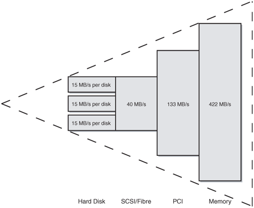
Once you get past the drives, look at the physical architecture of your system. Historically, as you move farther away in the signal chain from the processor, bandwidth decreases, which is shown in Figure 4-2. If you have a 800-MHz processor with 512 MB of PC133 SDRAM, talking over a 300 MHz bus that has a SCSI controller that can deliver up to 40 MB per second, and finally to a single drive that can sustain 15 MB per second, you have a pyramid with its smallest point, or tip, at the disk drive. Changing that picture a bit, changing one or more components of the system, or ensuring, say, a faster front side bus, might actually result in better performance. For example, does your solution need multiple SCSI controllers to fill your existing bus, or just a fatter, higher MHz 64-bit bus?
Next, break it down to your choice of hardware: what does each component bring to the table, and how can it possibly hinder you from a performance or availability standpoint? Very few people actually take the time to understand their hardware to this level, but in the availability and performance arenas, you must.
SQL Server has three types of disk I/O: random, readahead, and sequential. Random I/O is the 8k reads from a page, whether it is data or index. An example of a random I/O is a query with a WHERE clause. Readahead I/O issues 64k reads, and this maps to table and index scans. Table and index scans might be advantageous because the I/O cost of retrieving 64k when contiguously placed on the disk is close to that of retrieving 8k when paying the disk "seek" time between the next 8k. The final type of I/O, sequential I/O, is what the transaction log uses. Basically, you want the head to never pick up from the disk and just have it write to the log in a continuous stream. If the head has to pick up and go elsewhere, and then go back to the next position in the virtual log file, your writes to the log are slower, so reducing or eliminating latency for logs allows log records to be written faster. When SQL Server writes to a disk, it writes at the 8k page level (data or index). One of the main reasons SQL Server writes 8k pages is that these are database engine pages, not memory pages. 8k is a memory-address page boundary aligned requirement to use the high-speed I/O employed by SQL Server.
It is extremely important to consider the page size of 8k when designing schemas and indexes. Will all data from one row fit on a single page? Can multiple rows fit on a page? What will happen if you are inserting or updating data and you need to do a page split, either in data, or more to the point, in an index? Avoid page splits if at all possible because a page split causes another I/O operation that is just as expensive as a full 8k write. Keep this in mind with Unicode, as noted earlier, because it has slightly different storage characteristics.
Online transaction processing (OLTP) systems are heavy-duty read/write systems such as e-commerce systems. There are more random reads and writes with OLTP systems, and a safe assumption is at least 100 I/Os per second. The disk controller and cache should be matched to the ratio of reads and writes (see the next section, "Understanding Disk Cache"). For an OLTP system, it is potentially better to have a larger number of smaller drives to achieve better performance. One large disk (or LUN) over a smaller amount of disks might not result in the performance you want. To optimize the log, you might want to consider a dedicated controller set to 100 percent write as long as the transaction log is on a dedicated disk.
Caution
Do not attempt such a configuration unless you are certain that you are only using the write cache; otherwise you might encounter data corruption.
OLTP systems can quickly become log bound if your application performs many very small inserts, updates, and deletes in rapid succession (and you will see hotspotting on the log files if this is the case), so if you focus on the number of commits per second, ensure that the disk containing the log can handle this.
Tip
Consider analyzing your percentage of reads versus your percentage of writes. If you have more reads than writes, you might want more indexes, stripes with more spindles, and more RAM. If you have more writes than you do reads, large stripes and RAM will not help as much as more spindles and individual LUNs to allow the spindles to write without contention with other write I/O requests. Write cache can also help, but make sure you are completely covered when using the write cache for RDBMS files in general, and specifically, your log.
Planning for data warehouses is different than planning for OLTP systems. Data warehouses are largely based on sequential reads, so plan for at least 150 I/Os per second per drive due to index or table scans. The controller and cache should be set to heavy read. Put your data and indexes across many drives, and because tempdb will probably be heavily used, you should consider putting it on a separate LUN. Do not try to be a hero for object placement, because the query performance profile will change over time with use, addition of different data, new functionality, and so on. Achieving maximum performance would include having a dedicated performance and maintenance staff, but if that is not possible, design for maximizing I/O bandwidth to all disks and ensure proper indexes. Try to make the top 80 percent of your queries perform at optimal levels, and realize that 20 percent will be the outliers. You probably will not be able to have 100 percent of your queries perform optimally—choose the most used and most important, and then rank them on that basis. Log throughput is not as important, as data can be loaded in bulk-logged recovery mode, but it is still important for recoverability.
Taking technology out of the picture for a second, you need to understand the ratio of reads to writes in your individual application to be able to set the disk cache at the hardware level if possible (that is, you cannot do it if you are on a cluster and are using SCSI). If you have a 60 percent read, 40 percent write application, you could configure your cache to that ratio if your hardware supports this type of configuration. However, if you have more than one application or even multiple devices, say, attached to a SAN, optimizing your disk cache is nearly impossible if you have multiple applications sharing a LUN. Many SANs cache at the LUN level, but if they do not, your cache is shared among all LUNs, and you will only be able to do the best you can. This might also force you to have separate disk subsystems for different systems or types of systems to increase performance.
No discussion about availability and disks would omit a discussion on RAID. Over the years, RAID has stood for different things, but from a definition standpoint, it is the method of grouping your disks into one logical unit. This grouping of disks is called various things depending on your hardware vendor: logical unit, LUN, volume, or partition. A RAID type is referred to as a RAID level. Different RAID levels offer varying amounts of performance and availability, and each one has a different minimum number of physical disk drives required to implement it. There are many levels of RAID, and each manufacturer might even have its own variation on some of them, but the most popular forms of RAID are introduced here.
Important
Not all vendors support all the choices or options listed here for RAID, and some might even force you into a single, optimized method for their storage platform. Understand what you are purchasing.
Disk striping, or RAID 0, creates what is known as a striped set of disks. With RAID 0, data is read simultaneously from blocks on each drive. Because you only get one copy of the data with RAID 0, there is no added overhead of additional writes as with many of the more advanced forms of RAID. Read and write performance might be increased because operations are spread out over multiple physical disks. I/O can happen independently and simultaneously. RAID 0 spreads data across multiple drives, which means that one drive lost makes the entire stripe unusable. Therefore, for availability, RAID 0 by itself is not a good choice because it leaves you exposed without protection of your data. RAID 0 is bad for data or logs, but might be a good solution for storing online backups made by SQL Server before they are copied to tape. However, this is a potential risk, as you would need to ensure whatever process copies the backup to another location works, because losing a disk would mean losing your backup.
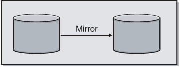
Disk mirroring, or RAID 1, is simple: a mirrored set of disks is grouped together. The same data is simultaneously written to both drives, and in the event of one drive failure, the other disk can service requests (see Figure 4-3). Some vendors support more than two disks in a mirror set, which can result in something like a triple or quadruple mirror. Read performance is improved with RAID 1, as there are two copies of the data to read from (the first serving disk completes the I/O to the file system), and unlike RAID 0, you have protection in the event of a drive failure. RAID 1 alone does have some high availability uses, which are detailed in the section "File Placement and Protection" later in this chapter. The disadvantage of mirroring is that it requires twice as many disks for implementation.
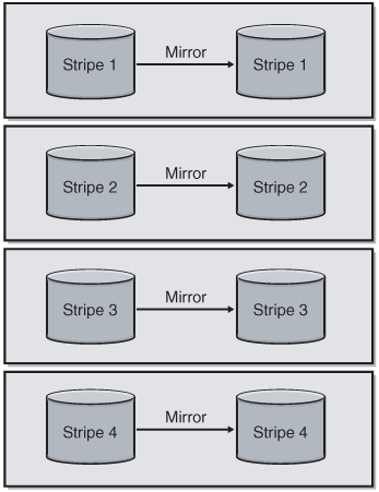
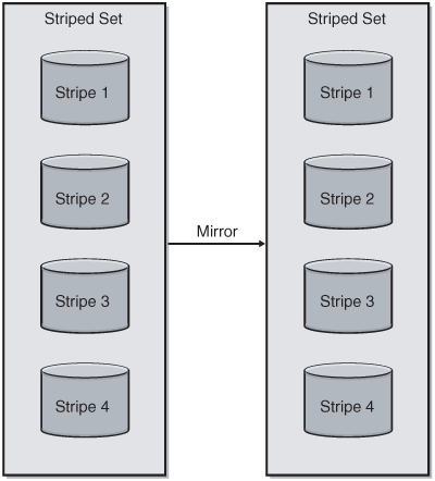
Striped mirrors are a hybrid of disks that are first mirrored with RAID 1, and then all mirrors are striped with RAID 0, as shown in Figure 4-4. Striped mirrors offer the best availability of the options presented in this chapter, as they can tolerate a drive failure easily and provides good fault tolerance. You could lose up to half of your disks without a problem, but losing the two disks constituting a mirror pair renders the entire stripe unreadable. Assuming no problems, you also have the ability to read from each mirror. When a failed disk is replaced, the surviving disk in the mirrored pair can often regenerate it, assuming the hardware supports this feature. Striped mirrors require a minimum of four drives to implement and can be very costly because the number of disks needed is doubled (due to mirroring). Striped mirrors are the most common recommendation for configuring disks for SQL Server.
Mirrored stripes are similar to striped mirrors, except the disks are first striped with RAID 0, and then each stripe is mirrored with RAID 1 (see Figure 4-5). This offers the second best availability of the RAID options covered in this chapter. You can tolerate the loss of one drive in each stripe set, as that renders that stripe set unusable. Your risk for failure goes up significantly once you encounter one drive failure. Mirrored stripes require a minimum of four drives to implement, and this solution is very costly, as you usually need at least two times the number of drives to get the physical space you need.
Striping with parity, shown in Figure 4-6, is also known as RAID 5, but it is parity that is not contained on one dedicated drive (that would be RAID 3); it is written across all of the disks and takes up the equivalent of one drive. RAID 5 is probably the most popular RAID level, as it is often the most cost effective in terms of maximizing drives for space.
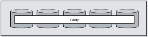
From an availability standpoint, RAID 5 is not the best—you can only tolerate the loss of one drive. When you lose a drive, your performance suffers, and once you lose more than one drive, your LUN no longer functions. RAID 5 uses the equivalent of one drive for storing a parity bit, which is written across all disks (hence only being able to lose one drive). RAID 5 also has slower write speeds, and so would not be appropriate for, say, a heavily used OLTP system. That said, many fast physical disks might mitigate (or mask) some RAID 5 performance issues. Caching capabilities of storage subsystems might also mitigate this so that it is no longer a point of consideration.
In a situation with unlimited financial and disk resources, striped mirrors give you better performance and reliability. In a limited disk scenario (for example, having only 12 or 16 disks), RAID 5 might be a faster or better implementation than striped mirrors. Of course, that would need to be evaluated.
A physical disk controller (hardware, not software) has two channels. Striped mirrors and mirrored stripes require both to mirror. RAID 5 could use two truly separate LUNs to separate out log and data, and you could access each individually, potentially increasing performance. If you have more than one disk controller and implement striped mirrors or mirrored stripes, you could get the same effect.
Assume you have 12 disks. With striped mirrors or mirrored stripes, you would only have six disks worth of space available because your storage is effectively halved. Even if the hardware can support simultaneous reads (that is, reading from both or all disks in the mirrored pair if you have more than two mirrors), you cannot have simultaneous writes from the application perspective because at a physical level, the hardware is performing simultaneous writes to maintain the mirror. Therefore, in some cases, RAID 5 with a smaller number of disks might perform better for some types of work.
Parity is a simple concept to grasp. Each physical disk has data (in megabytes or gigabytes), which then breaks down into smaller segments, ultimately represented by zeroes or ones. Picture a stripe, of say, 8 and you get the following:
1 0 1 0 0 0 1 1 (also known as A3 in hexadecimal)
Parity is simply the even or odd bit. For even parity, the parity bit would be 0 because if you sum the preceding numbers, you get four, and if you divide by two, there is no remainder.
Now that you understand the basics of parity, what does it buy you? Assume you lose the third disk, which would now make the example look like this: 1 0 x 0 0 0 1 1. If you then sum these numbers and divide by two, you now have odd parity. Therefore, you know you are missing a drive that must have contained a 1 to make the parity check.
Beyond the different types of RAID, there are two implementation forms: hardware-based and software-based. Hardware-based RAID is obviously implemented at a physical level, whereas software-based RAID is done after you start using the operating system. It is always optimal to have RAID done at a physical level.
For high availability, nothing can really beat a solution that allows you to geographically separate disks and maintain, say, two SQL Servers easily. This is more often than not a hardware-assisted solution. Remote mirroring is really the replication of storage data to a remote location. From a SQL Server perspective, the disk replication should be transactional based (as SQL Server is). If replication is not based on a SQL Server transaction, the third-party hardware or software should have a process (not unlike a two-phase commit) that ensures that the disk block has been received and applied, and if not, you are still maintaining consistency for SQL Server. If you are considering remote mirroring, ask yourself these questions:
Which disk volumes do you want to replicate or mirror?
What are the plans for placing the remote storage online?
What are the plans for migrating operations to and from the backup site?
What medium are you going to use for your disk replication? Distance will dictate this, and might include choices such as IP, Fibre Channel over specific configurations, and Enterprise Systems Connection.
What is the potential risk for such a complex hardware implementation?
Torn pages are a concern with remote disk mirroring. SQL Server stores data in 8k pages, and a disk typically guarantees writes of whole 512-byte sectors. A SQL Server data page is 16 of these sectors, and a disk cannot guarantee that each of the 16 sectors will always be written (for example, in the case of a power failure). If an error happens during a page write, resulting in a partially written page, that is known as a torn page. Work with your storage vendor to learn how they have planned to avoid or handle torn pages with your SQL Server implementation.
Each storage subsystem has a certain physical design with a high but limited number of disk slots. These are divided across multiple internal SCSI buses and driving hardware (processors, caches, and so forth), often in a redundant setup. If we now construct, for instance, a RAID 5 set but the same internal SCSI bus drives two spindles, that would be a bad choice for two reasons:
A failure on that internal bus would fail both disks and therefore fail the entire RAID 5 set on a single event. The same is true for two halves of a mirror, and it also applies to other redundant constructs of a storage subsystem.
Because RAID 5 uses striping, driving all spindles concurrently, two spindles on the same internal bus would need to wait on each other because only one device at a time on a single bus can be commanded. There is little waiting, as internally this happens asynchronously, but it still represents two consecutive operations that could have been one across all spindles at the same time, as is the intention of striping.
For these reasons, among others, some vendors do not offer these choices and abstract that to a pure choice in volume sizes, doing everything else automatically according to best available method given a particular storage solution design.
Windows supports three kinds of disks: basic, dynamic, and mount points.
A basic disk is the simplest form of disk: it is a physical disk (whether a LUN on a SAN or a single disk physically attached to the system) that can be formatted for use by the operating system. A basic disk is given a drive letter, of which there is a limitation of 26.
A dynamic disk provides more functionality than a basic disk. It allows you to have one volume that spans multiple physical disks. Dynamic disks are supported by both Windows 2000 and Windows Server 2003.
A mount point is a drive that can be mounted to get around the basic 26-drive letter limitation. For example, you could create a drive that is designated as F:SQLData, but maps to a local drive or a drive on a disk array attached to the server.
Caution
Only basic disks are supported for a server cluster using the 32-bit versions of Windows and SQL Server 2000 failover clustering. Basic disks are also supported under all 64-bit versions of Windows. Mount points are supported by all versions of Windows Server 2003 for a base server cluster, but only the 64-bit version of SQL Server supports mount points for use with failover clustering. Dynamic disks are not supported natively by the operating system for a server cluster under any version of Windows, and a third-party tool such as Veritas Volume Manager can be used. However, at that point, the third-party vendor would become the primary support contact for any disk problems.
Windows supports the file allocation table (FAT) file system, FAT32, and the NTFS file system. Each version of Windows can possibly update the version of the particular file system, so it is important to ensure that would not have any adverse affects in an upgrade process. For performance and security reasons, you should use NTFS.
Important
Only NTFS is supported for server clusters. FAT and FAT32 cannot be used to format the disks.
Tip
Keep in mind when that using Windows 2000 and Windows Server 2003, the 32-bit versions have a maximum limitation of 2 TB per LUN with NTFS. 64-bit versions remove this limitation, so if you are building large warehouses, you should consider 64-bit versions.
Warning
Do not enable compression on any file system that will be used with SQL Server data or log files; this is not supported in either stand-alone or clustered systems. For a clustered SQL Server, an encrypted file system is not currently supported. Windows Server 2003 clusters at the operating system level do support an encrypted file system. For updates, please consult http://support.microsoft.com.
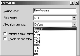
How you format your disks affects the performance of your disks used for SQL Server data. Disk subsystems optimized for a file server or for Exchange are not optimized for SQL Server. As discussed in the earlier section "Understanding How SQL Server Interacts with Disks," if your file system is not designed for SQL Server, you might not be able to get maximum performance. Whether using Computer Management or the command line format, set the NTFS block size appropriately (see Figure 4-7); 64K is recommended, and with 64-bit systems, this can even be set higher. If going beyond 64K, try it first on a test system. For SAN-based systems, make sure you work with your hardware vendor to ensure you are using the optimal stripe size settings for the type of RAID you employ.
Important
Make sure that you work closely with your preferred hardware vendor to ensure that the disks configured for your database are exactly the way you want them to be configured and that they are not optimized for other types of disk use. It is important to get the configuration documented for verification. In addition, if a problem occurs, you should have a guarantee from the vendor that the disks were configured properly. It can also help Microsoft Product Support Services or a third-party vendor assist you in the troubleshooting of any disk problems.
Another crucial factor in database availability and performance is where you place the data, log, and index files used by SQL Server, and what level of RAID you employ for performance and availability. This is another difficult piece in the disk puzzle, because it goes hand-in-hand with designing your storage at the physical hardware level. You cannot do one without the other. Especially at this stage, what you do not know about your application will hurt you. The physical implementation of your logical design, not unlike turning a logical schema into actual column names and data types, is a difficult process. They are both closely tied together, so one cannot be done in isolation from the other. For example, the logical design at some level has to take into account the physical characteristics of any proposed disk subsystem.
Note
In a failover cluster, all system databases are placed on the shared disk array. No databases are local to either node, otherwise a failover would be impossible.
On the other hand, the SQL Server 2000 binaries for both clustered and nonclustered systems are installed to local, internal drives in the system itself. This is a change from SQL Server 7.0. As in a cluster, you needed to put the binaries on the shared cluster disk. You should standardize where on each server SQL Server will be installed so that any DBA or administrator will know where SQL Server resides. In a clustered system, these binaries must exist in the same location.
For file placement of the system databases, it is easier to give general recommendations for both clustered and nonclustered systems. The only difference for a failover cluster versus a stand-alone SQL Server is that the system databases must all reside on the shared disk array in a cluster—they cannot be local to a server node. The following are the two main system databases for which you need to be concerned about file placement:
Tempdb. This system database is at the top of the list. Tempdb is often forgotten in the configuration equation, but can be a pivotal linchpin in the success of your SQL Server implementation because it serves as the scratch pad for the system. Tempdb is used to store all temporary tables (the ones that have a # prefix) and temporary stored procedures, and it is also used by queries for things like joins (which can create temporary work tables) and sorts. Tempdb is re-created every time SQL Server is restarted, so it is not a database that needs to factor into a backup and restore strategy. Tempdb, because it is write-intensive, would be better off placed on a RAID 1 LUN of its own if it is heavily used. RAID 5 might not buy you much with tempdb unless you could either give tempdb its own control channel or more working spindles. Combining tempdb with user databases is not a good idea if each individual database is heavily used.
Tip
Remember, tempdb also has a log file. Although it is rare, there are extreme cases in which it is possible to cause the performance problems for the tempdb log with enough transactional load. This would then require you to move this log to a separate disk or disk stripe in the same way you would for user data. Again, do not configure tempdb this way unless you have to.
Distribution. The distribution database is created when replication is installed. With merge and snapshot replication, the distribution database only stores status. However, with transactional replication, it is much more heavily used and must factor into any planning and performance. Hotspotting can potentially occur with RAID 5 if your disks are not quick enough to handle a heavy transactional volume with replication because of the overhead incurred to calculate and write the parity bit, so a striped mirror or mirrored stripe would probably help the distribution database. If your distribution database is located on the same server as your publication database and you have performance problems, you might try moving the distribution functionality to another server before you alter the disk subsystem.
Full-text indexes are also I/O intensive. In a cluster, these also obviously need to be on the shared disk array. In a nonclustered environment, you should not put the full-text index on the same drive or LUN as your log or data. Unless you have numerous spindles, your write performance suffers with RAID 5, so use some other form of RAID to increase your write and read performance.
Database backups are covered in depth in Chapter 9, "Understanding Your Backup and Restore Barriers," but they should be taken into account at the time of disk configuration. It might be cheaper and quicker to back up to disk, but if you are placing backups onto disk, or doing your primary backup to disk first, you need to account for that in your performance and storage requirements. You do not want to be performing a backup to a database and placing its resulting file on the same LUN or disk as the existing data file, as that reduces both your disk performance and available space.
For the system databases (master, model, tempdb, and so on), there is generally much less I/O than there is in a user database. Make sure that you protect them with at least RAID 1 for recovery and availability. Msdb is very important because it contains some settings that would be harder to restore without a good backup or having it available. Master is also important, but it can be rebuilt to an initial state with the REBUILDM command-line utility. You would still need a backup with your settings to restore over that, but there is no corresponding REBUILDM-like tool for msdb.
Where to place the user databases is always the million-dollar question, with no one-size-fits-all answer. Like all of high availability, it depends, based on all of the factors presented in this chapter.
As noted in Chapter 3, only one instance of SQL Server can access a given LUN (which might even have multiple logical drive letters configured on it), so it cannot be shared among instances. Similarly, the quorum, which is used by a server cluster (but not a majority node set server cluster—for more information, see Chapter 5), must be on its own disk because the base cluster resources need this disk. The minimum size recommendation for the quorum is 500 MB, and it might be larger if you keep the default configuration for the clustered MS DTC, which logs to the quorum disk. Again, MS DTC configuration is covered in Chapter 5. All of these factors affect any placement of databases and files in the cluster, so it must be planned for up front.
One of the biggest questions is when to use files and filegroups. Each database for SQL Server 2000 has a primary data file, and others, known as secondary data files, can also be used. In addition to the data files, there are files used for the transaction log. The primary data file has an extension of .mdf, secondary data files have an extension of .ndf, and log files have an extension of .ldf. Filegroups are exactly what they sound like: a group of files, but they are files that are grouped together. You cannot have files or filegroups used by more than one database. If you create a database named MyDatabase, only that database can use its corresponding .mdf and .ldf files.
Although there is a potential performance benefit to using multiple files and filegroups, the main reason you would consider implementing files and filegroups would be for easier administration. First and foremost, when you use multiple files for a database, whether log or data, they are filled proportionally. If you add a new file into the filegroup, it might show heavy I/O until it catches up with the other files. Second, files and filegroups allow you to deal with smaller portions of your database when doing maintenance, such as backups and restores, making maintenance windows easier to deal with. The success of files and filegroups is not to split up I/O bandwidth but to combine I/O bandwidth (that is, placing a file on each disk stripe for each filegroup). Scan density is king. SQL Server 2000 bases the degree of parallelism on the system load at the time the query execution plan is built. Readahead is based on the size of the buffer pool and the overall capacity of the I/O subsystem, so the number of files in a filegroup does not influence this.
However, as with any technology, there are always catches. Probably the biggest one for files and filegroups is that some maintenance within SQL Server 2000, such as DBCC INDEXDEFRAG, only works on a per-file basis. If you have an index that spans multiple files, you might encounter some fragmentation. DBCC DBREINDEX spans multiple files, but that is a trade-off for the potential performance impact and possible blocking due to employing it.
Caution
Do not use files and filegroups just for the sake of using them. If your database is small enough to easily be backed up and restored by your current strategy, files and filegroups might complicate things for you from an administrative perspective. In this case, if you decide to employ files and filegroups, it would generally be a performance improvement decision, which is not the usual case for implementing them—it is usually an administrative decision.
Once database file placement is worked out, one final step in the database configuration must be determined: the size of the files used for each user database, as well as tempdb. Again, what you do not know at this stage can hurt you when you move into production.
In versions of SQL Server prior to SQL Server 7.0, if you wanted to expand your database, you would have to do it by adding another segment. When you ran out of segments, you were out of luck. SQL Server 7.0 introduced the automatic growth functionality for a database, which allows a database to grow on the fly. This is a great feature, but it should be used with care, because if you accept the defaults, which are 10 percent growth and a file size of 1 MB (see Figure 4-8), you might be constantly chunking out to disk while the database is trying to continually expand as it is used.
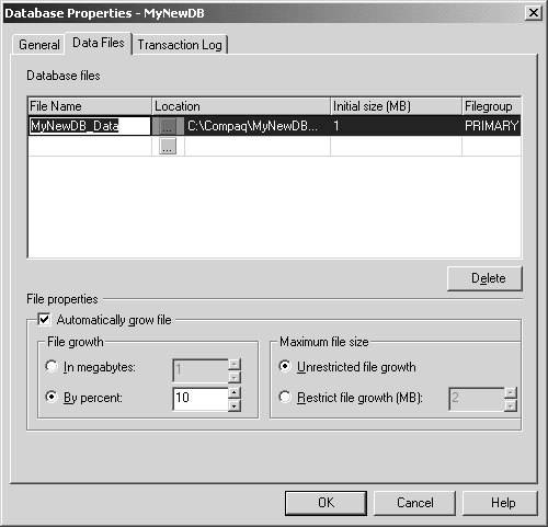
As the database grows, 10 percent growth might be sufficient, but in an initial, small database, this generally won’t fit your data curve. That creates a performance and potential availability problem because a large portion of your disk I/O is dedicated to expanding your disks, not just SQL Server usage. You can alter the growth properties of a database through Enterprise Manager, or use the ALTER DATABASE Transact-SQL command with the SIZE, MAXSIZE, UNLIMITED, or FILEGROWTH options. You should not set the file growth to UNLIMITED, as it allows the file chosen to grow until the disk is full. Some might want to set a maximum file size as well. If you do use the automatic growth, set a reasonable size, either by a percentage or physical size on disk, so that the database does not have to constantly grow.
Tip
Do not set the system databases to autogrow without good reason. Extra space in the system databases (with some exceptions, such as using transactional replication heavily in msdb where it stores history as well as the transactions) is generally not needed unless you are doing some sort of version upgrade or installing a service pack, and this would be detailed in the information supplied with the software you are upgrading to. Pick a size you are comfortable with when SQL Server is first installed.
User databases. What you probably care about most are the databases for your applications, whether third party or custom. The initial size of your database files should cover how much data you expect to have in the database for a time period of your determination plus some reasonable amount of growth.
Tempdb. Provides important functionality to SQL Server—especially for queries—so its size must be properly set. Do you know if your applications use tempdb heavily? If not, find out. If tempdb is continually expanding to meet your needs, you will always experience disk contention for tempdb, and if that file is placed in the same location as your data or log files, it has a domino effect on performance. Especially if you consolidate onto fewer SQL Servers, knowing how each application uses tempdb helps you determine the size of tempdb (it needs to accommodate all workloads), and also helps you determine if the workloads will actually work well together.
Important
You can always add more space to tempdb as needed. You can also take away space, but keep in mind that you cannot reduce the size of tempdb below the size at which you initially configured it when starting the SQL Server service without stopping and restarting SQL Server.
You can use SQL Server’s alerting capabilities to warn you when the file size for your database equals, exceeds, or falls below a certain size, as shown in Figure 4-9. This is a great way to notify you that there might be an upcoming problem, and if you have set a hard maximum size, you can take action, or let the alert take an action, such as issuing an ALTER DATABASE statement. See Chapter 14, or Chapter 15, for more information.
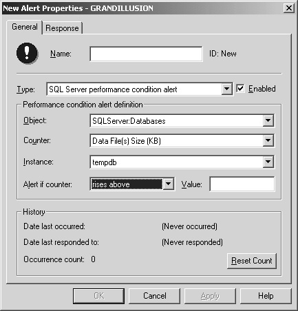
You can also decrease the size of your database and database files if, for example, you created them too large and have not experienced the growth you planned for. Like automatic growth, this should be done with care, as it might cause excessive disk I/O that will affect performance and possibly availability. To access the functionality in Enterprise Manager, right-click on a database, select All Tasks, and then select Shrink Database (see Figure 4-10).
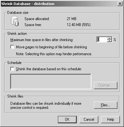
To shrink a database using Transact-SQL, use the DBCC SHRINKDATABASE command. DBCC SHRINKDATABASE shrinks all data and log files for a specified database. If you only want to shrink a particular data or log file, you can issue a DBCC SHRINKFILE command. Whether you shrink the entire database or just one file, it shrinks to the specified amount of free space you designate. You can also set the AUTO_SHRINK property ON or OFF for the database. If set to ON, this property periodically shrinks the database.
This section walks you through an example disk configuration. The goal is to understand the complexity of designing a disk array for a failover cluster that needs to take into account growth, performance, availability, and cost.
On the CD
A sample configuration worksheet can be found on the CD-ROM that accompanies this book. The file name is Disk_Configuration_Worksheet.doc, and it can be used to hypothesize the following scenarios or serve as a reference for the environment that you put together to become a part of your run book.
An application is going to be upgraded to use SQL Server 2000. Currently, it is on a stand-alone machine running SQL Server 7.0 with all disks local. For a primary form of availability, you have decided to use failover clustering, which means the disk array needs to be upgraded to one on the cluster-specific HCL (including new controllers if needed) and needs some careful consideration to be optimized for the new disk usage patterns.
Unfortunately, without DBA involvement, management has already purchased the hardware, and you are constrained by the following rules:
The array has already been purchased and has the capacity to hold 16 disks.
12 disks have been purchased, and unless necessary, no more will be bought. You would need to justify the extra disks.
Each disk is 36 GB with a speed of 10,000 rpm.
The array can be configured so that two disks are online spares.
The array is configured to talk over one channel, so splitting the array into, say, two disks of eight that might use more than one channel, is impossible.
Remember the location for tempdb and the quorum in the configuration.
Two years’ worth of growth should be factored in.
Important
Outside the context of this example, be aware that having no DBA involvement in the hardware decision making is not recommended. All DBAs should be involved with hardware procurement because these decisions affect not only your servers, but your job as well. You would much rather have people praise you for the performance and availability of a system than ask you why it is down or how long it takes to run a query ("I kick off my query before lunch because it takes too long, and the results are there when I get back").
As shown in Table 4-3, this application uses three databases:
Sales. This database is currently 50 GB, and has historically grown approximately 33 percent per year. This database uses tempdb heavily.
Billing. This database is currently 150 GB and has seen growth of about 25 percent per year.
Contacts. This database is currently 500 MB in size and grows roughly 10 percent per month.
Table 4-3. Databases Used by Sample Application
Database Name | Size at End of Year 1 (in GB) | Size at End of Year 2 (in GB) |
|---|---|---|
Sales | 66.5 | 88.5 |
Billing | 187.5 | 234.5 |
Contacts | 1.5 | 4.5 |
Raw Space Totals | 255.5 | 327.5 |
Assuming a 90:10 data-to-transaction log ratio, Table 4-4 shows the breakdown of file sizes to complement Table 4-3.
Table 4-4. Breakdown of File Sizes
Database Name | Size at End of Year 1 (in GB) | Size at End of Year 2 (in GB) |
|---|---|---|
Sales | 59.85 data/6.65 log | 79.65 data/8.85 log |
Billing | 168.75 data/18.75 log | 211.05 data/23.45 log |
Contacts | 1.35 data/0.15 log | 4.05 data/0.45 log |
Raw Space Totals | 229.95 data/25.55 log | 294.75 data/32.75 log |
Table 4-5 shows the total amount of raw drive space available.
There are more possible configurations, but the following four samples should give you a good idea of how challenging it is to configure a drive array. These examples all assume no use of files and filegroups. For your own edification, you might want to take these samples and try to think about how files and filegroups can be used with these configurations, and how they would change because of them.
None of the samples uses RAID 1+0/10/0+1. There are not enough drives to use that RAID level given the projected growth. None of these samples takes into account the archiving of data, either.
This sample (shown in Table 4-6) also adheres to the 12-drive limit. Quorum and tempdb each get their own RAID 1 LUN, and all of the data and logs are placed on a single RAID 5 LUN, meaning you will have a huge availability problem if the RAID 5 LUN fails. Notice that the total of 252 GB is not enough space for two years’ worth of growth, given the projections. The company has to buy more disks. No online spares means the company would have to stock drives in the event of drive failures.
This sample (shown in Table 4-7) also adheres to the 12-drive limit. The quorum and logs each get their own RAID 1 LUN (fixing the availability problem of Sample 1), and all of the data and tempdb are placed on a single RAID 5 LUN. Again, 252 GB is not enough space for two years’ worth of growth, given the projections. If the RAID 5 partition fails, you lose all of your databases, but you do have access to your logs in this case. You will have a serious performance problem because tempdb is on the same LUN as all of your data. Once more, the company has to buy more disks. No online spares means the company would have to stock drives in the event of drive failures.
Now that you know 12 disks are clearly not enough, there is a decision to buy two more disks. This time (Table 4-8), with 14 disks, you decide to split tempdb onto its own RAID 1 set to increase performance. You are still short on data growth space for two years’ worth of growth. As with Sample 2, your logs are split out, so you do have increased availability, but because all your logs are on one RAID 1 set, you will not get the maximum performance from your logs. You still need more drives. No online spares means the company would have to stock drives in the event of drive failure.
The decision to max out the drive array at 16 disks is made. This configuration (Table 4-9) gives the proper amount of drive space, but you could not add online spares even if you wanted to.
This sample (Table 4-10) shows you from a maximum performance and space standpoint how you could potentially configure a disk subsystem if you have enough drives. This does not address files and filegroups, manageability, and hotspotting, which would come from knowing your data—this just handles space and base performance from a 10,000-foot view.
Proper disk configuration ensures that your SQL Server implementations are highly available and deliver the performance that you need from your disk subsystem. Planning can prevent future problems due to growth, performance, or disk availability. It is sometimes better to buy enough disk storage space—that is, the physical enclosure space—up front than it is to buy all of your disks at once. If your disk solution supports dynamic or easier growth, you can maximize your hardware investment, as you have planned for all of your growth but can expand when you need it. Using multiple controllers to support different types of reads and writes might be optimal, but it is expensive. Whatever you buy and implement affects every other aspect of your SQL Server and application solution.