
In this chapter, we will look at a useful technique that combines several functions into a single formula. We can call it a megaformula. In other words, we have one or more functions nested inside other functions. The use of megaformulas is a contentious issue. Some people claim that having multiple intermediate formulas results in a clearer understanding of what is happening as compared to having a single complex formula. As a user, it’s your call as to whether megaformulas would be helpful in your scenario.
What Is a Megaformula?
Many times, we use intermediate formulas in a worksheet to produce a result that we want. In other words, we have formulas that depend on other formulas. Once all these formulas are working correctly, we can remove all of these intermediate formulas and combine them to create a single large, complex formula. We can call such a formula a megaformula.
Advantages of Megaformulas
- 1.
They use fewer cells, resulting in faster recalculations. This of course will depend on the specific scenario and the formulas used.
- 2.
You can impress your boss and colleagues with your ability to build complex formulas.
Disadvantages of Megaformulas
- 1.
The formula probably will be difficult to understand or modify, even for the creator of the megaformula.
Examples of Megaformulas
Now, let us look at some examples.
Dynamic Lookup Using INDEX MATCH Functions
INDEX function with MATCH function
- 1.
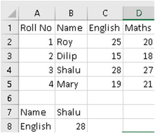
The first argument to the INDEX function is the search range from A1 to D5. Note that we have used absolute reference for the search range.
- 2.
The second argument to the INDEX function is MATCH(B7,$B$1:$B$5,0), Here, we are telling the MATCH function to find the value in cell B7 (Shalu) in the range B1 to B5. This will return 4, as the value Shalu occurs in the fourth row of the search range B1 to B5.
- 3.
The third argument to the INDEX function is MATCH(A8,$A$1:$D$1,0). Here, we are telling the MATCH function to find the value in cell A8 (English) in the range A1 to D1. This will return 3, as the value English occurs in the third column of the search range A1 to D1.
- 4.
Now that we have the row and column references, we tell the INDEX function to return the cell value at the intersection of the fourth row and third column. This is the value in cell C4.
As you saw in this example we have the two MATCH functions nested inside the INDEX function.
Create a Name Using the First Letter of the First Name and the Last Name
Name example
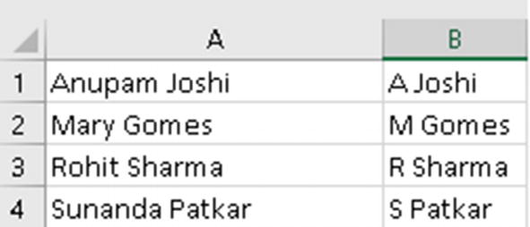
In cells A1 to A4 we have names consisting of first name and last name. In cell B1 we have used the formula =LEFT(A1,1) & MID(A1, FIND(" ", A1), LEN(A1)). Copy the formula in cell B1 to cells B2 to B4.
- 1.
First, the function LEFT(A1,1) is evaluated. This will return the first character from cell A1, which is the first letter from the first name. This will return the value A.
- 2.
Next, the formula FIND(" ", A1) is evaluated. This will find the position of the first space in cell A1. This will return 7.
- 3.
The value returned in step 2 is used in the MID function as follows: MID(A1, 7, LEN(A1)). Here, we are saying return the text starting from position 7 till the end of the string (the end of the string is given by the function LEN(A1)). This will return the value Joshi.
- 4.
The value returned in step 3 is joined using the ampersand (&) to the value returned in step 1.
Create a Name Consisting of Only First and Last Name
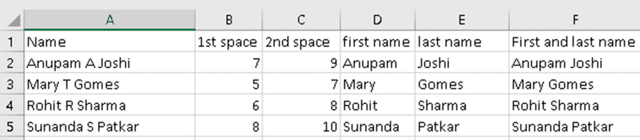
How Excel will look with intermediate formulas
Formula Used for Cells in Figure 13-3
Cell Reference | Formula | Explanation |
|---|---|---|
B2 | =FIND(“ ”, A2) | Find the position of the first space in cell A1. |
C2 | =FIND(“ ”, A2, B2+1) | Find the position of the second space in cell A1. |
D2 | =LEFT(A2,B2-1) | Return the first name. |
E2 | =MID(A2,C2+1,LEN(A2)) | Return the last name. |
F2 | =D2 & “ ” &E2 | Combine the first name and last name separated by a space. |
Copy the formulas in cells B2 to F2 to cells B3 to F5.
Now let us create a megaformula to eliminate the intermediate formulas. Enter the following formula in cell H2:
=MID(A2,1,FIND(" ", A2)-1) & " " & MID(A2,FIND(" ", A2, FIND(" ", A2)+1)+1,LEN(A2)). Copy this formula to the other cells.
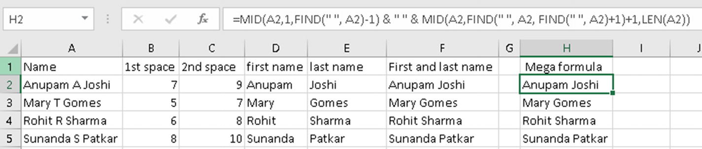
First and last names using a megaformula
Reverse a Text String
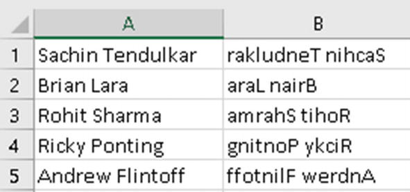
Reverse a string
In cell B1, we have used the formula =TEXTJOIN("", 1, MID(A1, ABS(ROW(INDIRECT("1:" & LEN(A1))) - (LEN(A1) + 1)), 1)) . For those of you who do not have Microsoft 365, after entering the formula, press Ctrl+Shift+Enter, as this is an array formula. For those of you who have Microsoft 365, you need to just press the Enter key, even for an array formula. Copy the formula in B1 to cells B2 to B5.
- 1.
First, the formula will find the length of the string.
- 2.
Based on the length of the string, the individual positions will be determined in reverse order. The part of the formula that does this is ABS(ROW(INDIRECT("1:" & LEN(A1))) - (LEN(A1) + 1)).
- 3.
Next, each character is extracted using the MID function, starting from the last character to the first character.
- 4.
Finally, each character extracted in step 3 is concatenated using the TEXTJOIN function.
Summary
In this chapter, we looked at megaformulas. As always, I suggest you try out the examples from this chapter using your own data and also using the different options for the arguments. This will give you more clarity regarding how the functions actually work.
In the next chapter, we will look into the interesting topic of array formulas.