
In this chapter, we will look into what named ranges are, how to create one, and what their benefits are. Then, we will look into a powerful but often overlooked feature of Excel, the Excel table.
Named Ranges
instead of regular cell references in formulas,
to define the source for graphs, and
to define the data validation source.
Advantages of Named Ranges
Formulas become easier to understand and debug.
The creation of complicated spreadsheets becomes easy.
They help to simplify your macros.
Create a Named Range
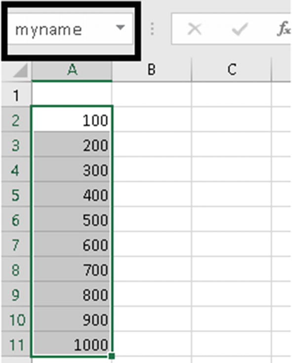
Create a named range
Name Manager
- 1.
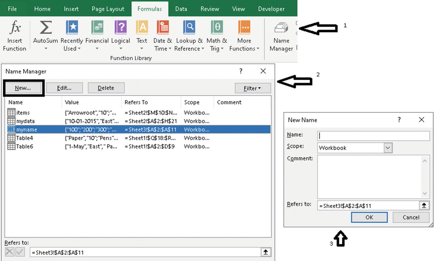
Click on the Formulas tab in the ribbon, as shown by arrow 1.
- 2.
Click on Name Manager. You get the Name Manager, as shown in Figure 5-2 at arrow 2.
- 3.To create a new named range, click on New in the Name Manager window. You get the New Name window, as shown by arrow 3 in Figure 5-2. Here you can supply the following:
The name for the range
The scope of the named range. The default is workbook, which means the name can be referenced anywhere in the current workbook. The other scope is the sheet name, which means the name can be referenced only in the selected worksheet. To use a named range with a worksheet scope throughout the workbook, you need to put the name of the worksheet before the named range; e.g., Sheet1!myNamedRange.
Refers To is the range the name refers to. This can also be a literal value or a formula.
Rules for Creating Names
It can start with a letter or an underscore (_).
The name cannot exceed 255 characters.
Spaces are not allowed as part of a name.
Names cannot be the same as a cell reference, such as A$35.
You cannot use C, c, R, or r as a defined name—they are used as selection shortcuts.
SalesReps or sales_reps
CompanyNames or company_names
StudentsList or students_list
Benefits of Named Ranges
Names are easier to remember when typing formulas.
Formulas are easier to read when using named ranges.
You can jump to a specific location easily without the need to remember the row and column address.
Excel Tables
Tables allow you to easily manage and analyze a group of related data. You can turn a range of cells into an Excel table. Every Excel table that you create is automatically named by Excel. You can change the table name to your liking. So, you can see that a table name is like a named range. Tables are a powerful but often overlooked feature of Excel.
Benefits of Using Excel Tables
Excel keeps track of the range used for the table. This frees you from having to manually track row/column additions/deletions.
Users typically face a problem when working with a large data set. The column headers tend to disappear as you scroll down the data. Tables solve this problem. When the column headers scroll off, Excel replaces the names of the worksheet columns with table headers. This will happen only when a cell in the table is selected.
Excel tables can have a dedicated Total row, which is automatically updated as data is added/modified/deleted.
When you enter a formula in a column of an Excel table, the formula is automatically copied throughout the column. You do not have copy and paste the formula to other cells.
Sort and filter options are available the moment you create an Excel table.
Creating a Table
- 1.
Select a cell in the data that you wish to convert to an Excel table.
- 2.
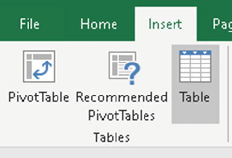
Select the Table option, as shown in Figure 5-3. The Table button is in the Insert tab.
Create a table
- 3.
In the Create Table dialog box, the range for your data should automatically appear. Depending on the type of data in the table, the My table has headers option may or may not be checked. You can adjust the range and uncheck or check the box if required. Figure 5-4 shows the Create Table dialog box. Click OK to accept changes.

Create Table dialog box

Excel table
As you can see, the data is nicely formatted with filters automatically applied to the column headers.
Styling a Table

Applying styles to table
In Figure 5-6, the large black box shows some of the styles available. To see more styles, click on the arrow in the inner small black box.
Renaming a Table
Rename a table
- 1.
Ensure that the active cell is in the table to be renamed.
- 2.
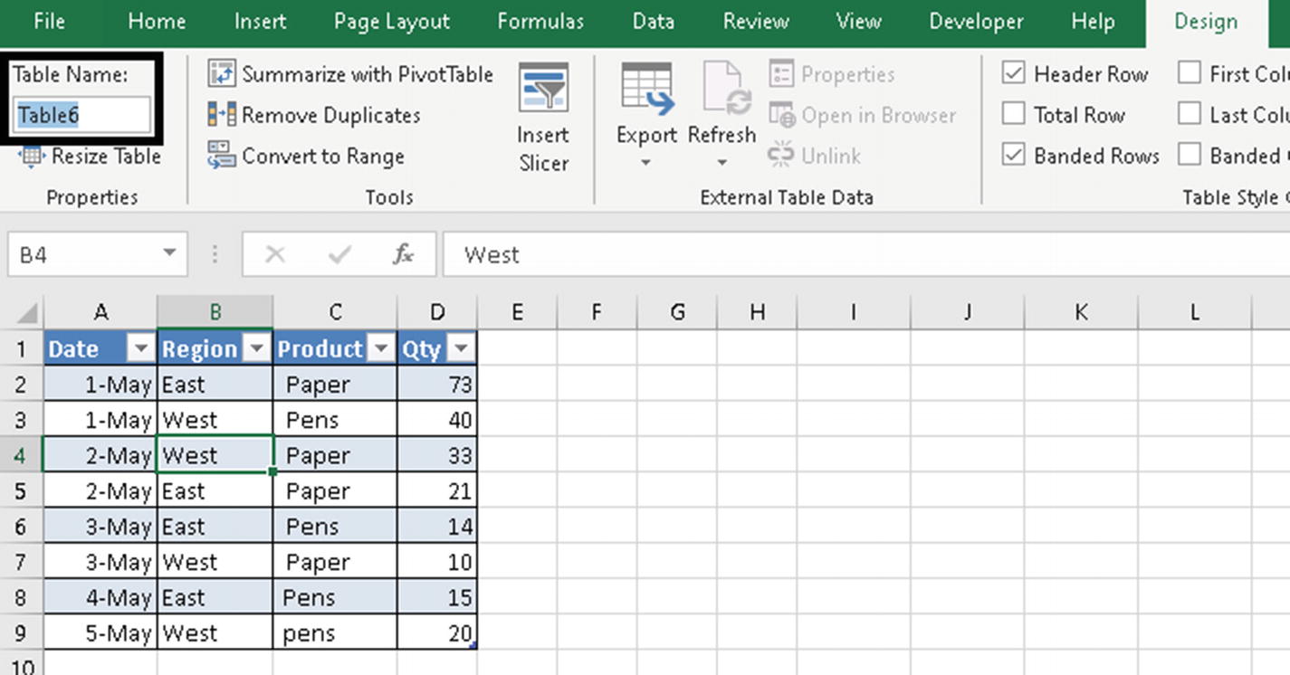
Click on the Design tab in the ribbon bar.
- 3.
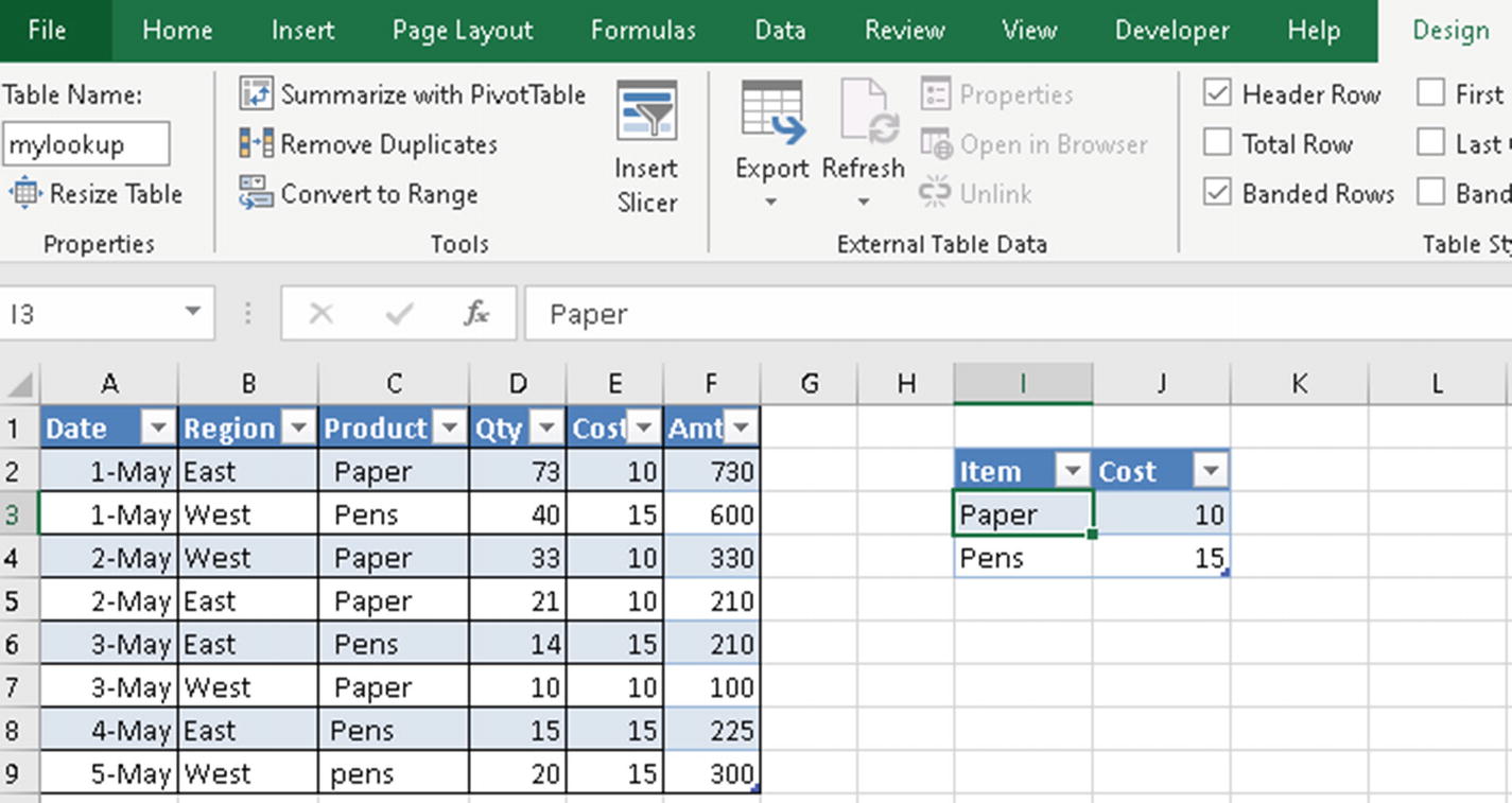
By default, Excel gives a name to every table that you create. To change the name, click on the Table Name box highlighted by the black box in Figure 5-7. Change the table name and press the Enter key so that the new name is used.
Table names follow the same rules as named ranges.
Adding a Reference to Another Table
How to refer to one table from another in a formula
In Figure 5-8, we have created a lookup table in the cells I3 to J4. This lookup table contains the items and their cost per unit. We have named this lookup table mylookup, as can be seen in Figure 5-8.
First, we add a new column named Cost in column E. The moment you enter “Cost” in cell E1 and press the Enter key, the new column gets automatically added to the existing table. Similarly, add the value Amt in cell F1.
You might be wondering what the [@Product] in the VLOOKUP formula is. Well, it refers to the value in the Product column for the current row.
Similarly, for the second argument of VLOOKUP, we have used the lookup table name instead of a cell range.
[@Qty] refers to the value from the Qty column for the current row.
[@Cost] refers to the value from the Cost column for the current row.
Excel Table References
Referring to | Referred in Formula as | Comments |
|---|---|---|
The entire table | =Table1 | We use the table name to refer to the entire table. |
The current row | =Table1[@Qty] | We prefix the column name with an @ sign to indicate the current row. |
Table headers | =Table1[#Headers] | This is used when you want to refer to only the table headers in your formula. |
Adding a Total Row to the Table

Total row in table
- 1.
Ensure that a cell in the table is selected.
- 2.
Select the Design ribbon and then click on Total Row, as shown by the black box in Figure 5-9.
- 3.
You get the total for the Amt column. This is the default behavior.
- 4.
The formula that Excel will automatically put in cell F10 is =SUBTOTAL(109,[Amt]). We will look into the SUBTOTAL function in the chapter on aggregate functions.
Your table should look like the one in Figure 5-9 after adding the Total row.
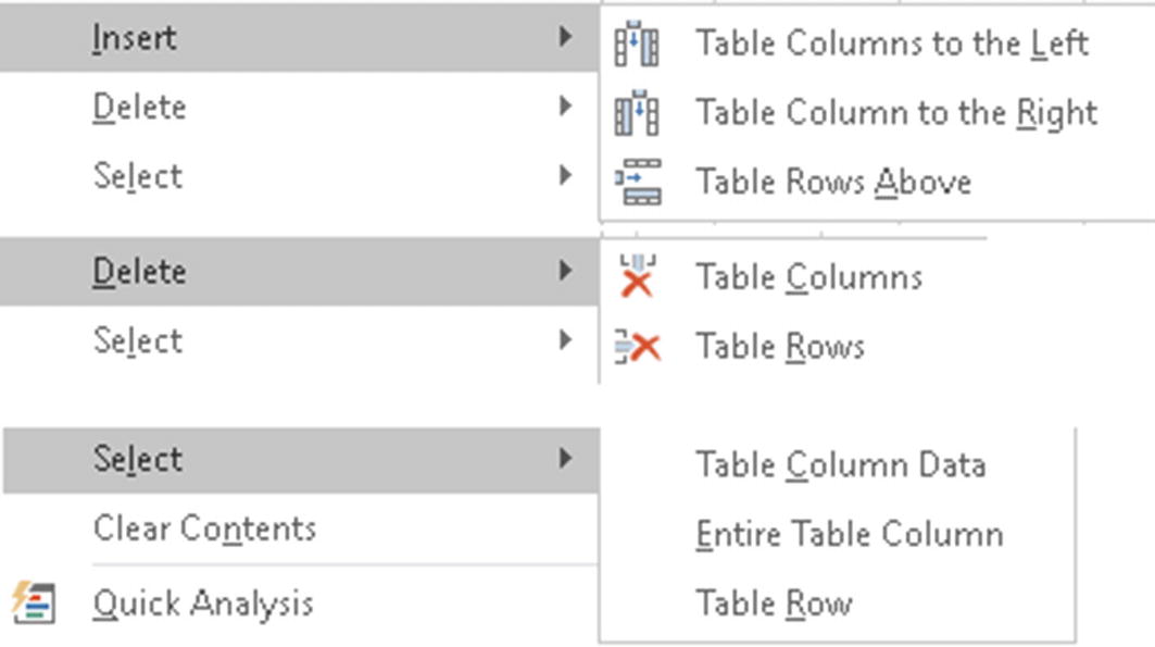
Excel table options insert/delete/select
Summary
To summarize, in this chapter we looked at named ranges and Excel tables. As always, I suggest you try out the examples from this chapter using your own data and also using the different options for the arguments. This will give you more clarity regarding how the functions actually work.
In the next chapter, we will look at lookup functions.