
In this chapter, we will look into some of the most commonly used finance functions provided by Excel for use in financial calculations. So, let us began.
FV Function
The FV function returns the future value of an investment that has periodic constant payments and a constant interest rate.
Syntax
- The first argument is the interest rate for the period. Here, it is assumed that payment is made once per year. If the payment period is different, divide the rate accordingly. So,
if payment is monthly, divide the rate by 12; or
if payment is quarterly, divide the rate by 4.
- The second argument is the total number of payment periods. Here again, if the payment period is different, the number of payment periods has to be entered accordingly. So,
if payment is monthly, the number of periods will be 12; or
if payment is quarterly, the number of periods will be 4.
The third argument is the payment made each period. If this argument is omitted, the present value (which is the fourth argument) must be given.
The fourth argument is optional. The fourth argument specifies the present value. If this argument is omitted, it is considered to be zero.
- The fifth argument is the type. This argument is optional. This argument specifies if the payment is made at the beginning or the end of the period. It can have one the following values:
0 – Indicates payment is made at the end of the period. The value 0 is used if this argument is omitted.
1 – Indicates payment is made at the beginning of the period.
Example
FV function
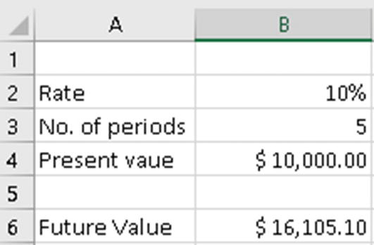
In Figure 11-1, we are trying to get the future value of $10,000 invested at 10 percent yearly interest for a period of five years. The formula used in cell B6 is =FV(B2,B3,,-B4). The value returned is $16,105.1. What this indicates is that for an amount of $10,000 invested for five years at 10 percent interest compounded annually, the maturity amount will be $16,105.1.
Let us look at another example. Enter the following formula in a blank cell: =FV(10%/12,60,-1000). Here, we are trying to find out the future value of an investment of $1,000 per month for a period of five years. The interest is 10 percent per year, and each payment is made at the start of the month. The return value is $77,437.07.
Since the payments are made monthly, the annual interest rate of 10 percent has been converted into a monthly rate (=10%/12), and the five-year period has been input as a number of months (60).
Also, since the monthly payments are paid out, we have used -1000 as input to the function.
PV Function
The PV function returns the present value of an investment based on a series of future payments.
Syntax
- The first argument is the interest rate for the period. Here, it is assumed that payment is made once per year. If the payment period is different, divide the rate accordingly. So,
if payment is monthly, divide the rate by 12; or
if payment is quarterly, divide the rate by 4.
- The second argument is the total number of payment periods. Here again, if the payment period is different, the number of payment periods has to be entered accordingly. So,
if payment is monthly, the number of periods will be 12; or
if payment is quarterly, the number of periods will be 4.
The third argument is the payment made each period. If this argument is omitted, the future value (which is the fourth argument) must be given.
The fourth argument is optional. The fourth argument specifies the future value. If this argument is omitted it is considered to be zero.
- The fifth argument is the type. This argument is optional. This argument specifies if the payment is made at the beginning or the end of the period. It can have one of the following values:
0 – Indicates payment is made at the end of the period. The value 0 is used if this argument is omitted.
1 – Indicates payment is made at the beginning of the period.
Example
PV function
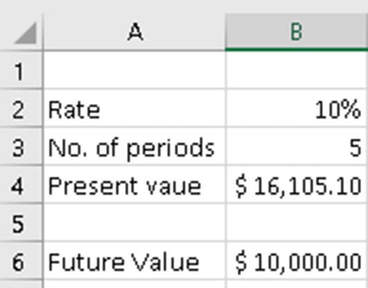
In Figure 11-2, we are trying to get the present value of $16,105.1 invested at 10 percent yearly interest for a period of five years. The formula used in cell B6 is =PV(B2,B3,,-B4). The value returned is $10,000.
Let us look at another example. Enter the following formula in a blank cell: =PV(10%/12,60,,-5000). Here, we are trying to find out the present value of an investment that has a total value $5,000 after making monthly payments for five years. The interest is 10 percent per year, and each payment is made at the start of the quarter. The return value is $3,038.94.
Since the payments are made monthly, the annual interest rate of 10 percent has been converted into a monthly rate (=10%/12), and the five-year period has been input as a number of months (60).
Also, since the monthly payments are paid out, we have used -5000 as input to the function.
PMT Function
The PMT function is used to calculate the periodic payment value. This is generally used to calculate the EMI of a loan.
Syntax
The first argument is the interest rate for the period.
The second argument is the number of periods over which the payment/investment is to be made.
The third argument is the present value of the loan or investment.
The fourth argument is optional. It specifies the future value of the loan or investment at the end of all payments. If this argument is omitted, it is considered to be zero.
- The fifth argument is the type. This argument is optional. This argument specifies if the payment is made at the beginning or the end of the period. It can have one the following values:
0 – Indicates payment is made at the end of the period. The value 0 is used if this argument is omitted.
1 – Indicates payment is made at the beginning of the period.
Example
For this example, the PMT function is used to calculate the monthly payments on a loan of $500,000 that is to be paid off in full after five years. Interest is charged at a rate of 10 percent per year, and the payment to the loan is to be made at the end of each month. Enter the following formula in a blank cell: =PMT( 10%/12, 60, 500000).
As the payments are made monthly, the annual interest rate of 10 percent is divided by 12 to convert it into the monthly rate, and the period of five years is converted in months (60).
The future value and type arguments are omitted as the future value is zero, and the payment is to be made at the end of the month.
The value returned from the function is negative, as this represents an outgoing payment for repayment of the loan taken.
IPMT Function
The IPMT function returns the interest payment for a specific period of a loan or investment where the payments and interest rates are constant.
Syntax
The first argument is interest rate for the period.
The second argument is the period for which you want to find the interest. This value should be between 1 and the total number of periods.
The third argument is the total number of periods.
The fourth argument is the present value of the loan or investment.
The fifth argument is optional. It is the future value at the end of the number of periods specified in the third argument. If this argument is omitted, future value is taken as zero.
- The sixth argument is the type. This argument is optional. This argument specifies if the payment is made at the beginning or the end of the period. It can have one the following values:
0 – Indicates payment is made at the end of the period. The value 0 is used if this argument is omitted.
1 – Indicates payment is made at the beginning of the period.
Example

IPMT function
In Figure 11-3, we have a loan amount of $50,000 to be paid back in twelve monthly installments. The interest rate is 10 percent. In cell B4 we have used the formula =IPMT($B$2/12,A4,$B$3,$B$1). This will return the value $416.67. This is the interest part of the loan installment for the first month. Copy the formula in cell B4 to cells B5 to B15. These will return the interest parts of the loan installments for the respective months. As you can see, the interest part keeps reducing as we move toward the end of the payment period.
PPMT Function
The PPMT functions returns the principal payment for a specific period of a loan or investment where the payments and interest rates are constant.
Syntax
=PPMT(rate, period, number of periods, present value, [future value], [type])
The first argument is the interest rate for the period.
The second argument is the period for which you want to find the principal paid. This value should be between 1 and the total number of periods.
The third argument is the total number of periods.
The fourth argument is the present value of the loan or investment.
The fifth argument is optional. It is the future value at the end of the number of periods specified in the third argument. If this argument is omitted, future value is taken as zero.
- The sixth argument is the type. This argument is optional. This argument specifies if the payment is made at the beginning or the end of the period. It can have one the following values:
0 – Indicates payment is made at the end of the period. The value 0 is used if this argument is omitted.
1 – Indicates payment is made at the beginning of the period.
Example
PPMT function
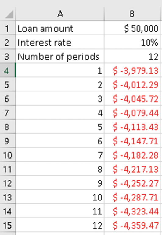
In Figure 11-4, we have a loan amount of $50,000 to be paid back in twelve monthly installments. The interest rate is 10 percent. In cell B4 we have used the formula =PPMT($B$2/12,A4,$B$3,$B$1). This will return the value $3,979.13. This is the principal part of the loan installment for the first month. Copy the formula in cell B4 to cells B5 to B15. These will return the principal parts of the loan installments for the respective months. As you can see, the principal part keeps increasing as we move toward the end of the payment period.
RATE Function
to pay off a loan, or
to reach a target amount of investment.
Syntax
The first argument is the number of periods over which the loan/investment is to be paid off.
The second argument is the fixed amount to be paid for each period.
The third argument is the present value of the loan/investment.
The fourth argument is the future value; this argument is optional. If omitted it is considered as zero.
- The fifth argument is the type. This argument is optional. This argument specifies if the payment is made at the beginning or the end of the period. It can have one the following values:
0 – Indicates payment is made at the end of the period. The value 0 is used if this argument is omitted.
1 – Indicates payment is made at the beginning of the period.
The sixth argument is the estimate of the interest rate. This argument is optional. If omitted, it is assumed to be 10 percent.
Example
In this example, we are trying to calculate the interest rate to pay off a loan amount of $80,000 over a period of four years with a fixed monthly payment of $2,000. Enter the following formula in a blank cell: =RATE(4*12,-2000,80000). This will return 0.77 percent. Since this is the monthly rate, we need to convert it into an annual rate by multiplying it by twelve. So, change the formula you just entered to make it look like the following formula: =RATE(4*12,-2000,80000) *12. This will return 9.24 percent, which is the annual rate.
NPER Function
The NPER function is used to calculate the number of periods required to pay off a loan wherein the periodic payment amount and interest rate are constant.
Syntax
The first argument is the interest rate.
The second argument is the periodic payment amount.
The third argument is the present value of the loan.
The fourth argument specifies the future value of the loan. This argument is optional. If omitted, this value is taken as zero.
- The fifth argument is the type. This argument is optional. This argument specifies if the payment is made at the beginning or the end of the period. It can have one the following values:
0 – Indicates payment is made at the end of the period. The value 0 is used if this argument is omitted.
1 – Indicates payment is made at the beginning of the period.
Example
In this example, we try to calculate the number of periods required to pay off a loan of $500,000 at the rate of $120,000 per year. The interest rate charged is 10 percent. The payment is made at the start of the period.
The payment for the loan is a negative value (-10000), as this represents an outgoing payment.
The payments are made monthly, so the annual interest rate of 10 percent is converted into a monthly rate (10%/12).
The type argument is set to 1, as the payment is to be made at the beginning of each month.
The value returned from the NPER function is in months, which is 64.24 months, which is the same as 5.35 years.
NPV Function
The NPV function is used to calculate the net present value of an investment based on a discount rate and a series of future payments (negative values) and incomes (positive values). Here, the cash flows are assumed to be periodic.
Syntax
The first argument is the discount rate.
Value1 to value254 is the list of numeric values representing payments and incomes.
Negative values are treated as payments.
Positive values are treated as income.
Example

NPV function
In Figure 11-5, first let us look at the formula in cell B9, which is =NPV(B2,B3:B8). In this formula, the discount rate comes from cell B2 and the value arguments come from cells B3 to B8. This function gives the result $50,166.21. In this example, the initial investment of $100,000 (shown in cell B3), is made at the end of the first period. Therefore, this value is included as the first value argument to the NPV function.
In Figure 11-5, the formula in cell C9 is =NPV(C2,C4:C8)+C3. In this formula, the discount rate comes from cell C2 and the value arguments come from cells C4 to C8. This function gives the result $55,182.83. In this example, the initial investment of $100,000 (shown in cell C3) is made at the start of the first period. Therefore, this value is not included as the first value argument to the NPV function. Instead it is added to the NPV formula.
IRR Function
The IRR function returns the internal rate of return for a series of periodic cash flows. The internal rate of return (IRR) is widely used in business to choose between investments, as it indicates the profitability of an investment.
Syntax
The first argument is an array of values or a reference to cells that contain numbers for which you want to calculate the internal rate of return. The values list must contain at least one positive value and one negative value to calculate the internal rate of return.
The second argument is the initial guess of the expected IRR. This argument is optional. Starting with a guessed value given by the user, the IRR function cycles through the calculation until the result is within 0.00001 percent accuracy. If this argument is omitted, Excel will take it to be 10 percent. If the IRR function cannot find a working result after twenty tries, the #NUM! error value is returned.
Example

IRR function
In Figure 11-6, cell A2 shows the initial investment. Since this is a cash outflow, the value is negative. Cells A3 to A7 contain the expected income from the first year to the fifth year. In cell A9, we have used the formula =IRR(A2:A5). Here, we are trying to find out the internal rate of return for the initial investment of $-100,000 after three years. The value returned is -11 percent. In cell A10, we have used the formula =IRR(A2:A7). Here, we are trying to find out the internal rate of return for the initial investment of $-100,000 after five years. The value returned is 13 percent. So, you can see that the IRR is negative after three years but is positive after five years. Since we have not used the guess argument, Excel takes 10 percent as the starting point for the iteration of up to twenty attempts to achieve the required accuracy. Being more accurate will make Excel faster and reduce the risk of getting a #NUM! error, but in most circumstances will not change the outcome of the result.
XIRR Function
The XIRR function returns the internal rate of return for a series of cash flows that are not periodic.
Syntax
The first argument is an array of values or a reference to cells that contain numbers for which you want to calculate the internal rate of return. The values list must contain at least one positive value and one negative value to calculate the internal rate of return.
The second argument is the series of dates corresponding to the values supplied.
The third argument is the initial guess of the expected IRR. This argument is optional. Starting with the guessed value given by the user, the IRR function cycles through the calculation until the result is within 0.00001 percent accuracy. If this argument is omitted, Excel will take it to be 10 percent. If the IRR function cannot find a working result after twenty tries, the #NUM! error value is returned.
Example
XIRR function
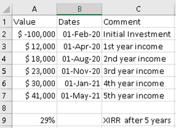
In Figure 11-7, in cell A9 we have used the formula =XIRR(A2:A7,B2:B7). This will return a value of 29 percent.
XNPV Function
The XNPV function is used to calculate the net present value of an investment where the cash flows are not periodic.
Syntax
The first argument is the discount rate to be applied to the cash flows.
The second argument is a series of cash flows. Negative values are treated as outflows and positive values are treated as inflows.
The third argument is the series of dates for the cash flows. The length of the date series should be the same as the values series.
Example

XNPV function
In Figure 11-8 in cell B8 we have used the formula =XNPV(B2,B3:B8,C3:C8). This will return the value $94,332.65.
Summary
In this chapter, we had a look at some of the financial functions available in Excel. As always, I suggest you try out the examples from this chapter using your own data and also using the different options for the arguments. This will give you more clarity regarding how the functions actually work.
In the next chapter, we will look into handling errors that occur in Excel formulas.