Chapter 3: DirectQuery Optimization

Until now, we have looked at Power BI performance from a relatively high level. You have learned which areas of Power BI performance can be impacted by your design decisions and what to consider when making these choices. These decisions were architectural, so were about choosing the right components to ensure the most efficient movement of data to suit your data volume and freshness requirements.

However, this knowledge alone is not sufficient and will not guarantee good performance. With the gateways in the previous chapter, we saw how a single component of the solution can be configured and optimized quite heavily. This applies to most of the other areas of Power BI, so now we will begin to deep dive into how specific design decisions in each area affect user experience and what configurations should be avoided.

In Chapter 2, Exploring Power BI Architecture and Configuration, we looked at storage modes for Power BI datasets and learned about Import and DirectQuery. In this chapter, we will look specifically at the DirectQuery storage mode. Power BI reports issue queries in parallel by design. Each user interaction on the report can trigger multiple queries. You can have many users interacting with DirectQuery reports that use the same data source. This potentially high rate of queries to the external source must be taken into consideration when building DirectQuery models.

We will look at data modeling for DirectQuery models to reduce the chance of overwhelming the data source. You will learn how to avoid Power BI and the data source performing extra processing. We will learn about the settings available to adjust DirectQuery parallelism. We will also look at ways to optimize the external data source and leverage its strengths to handle the type of traffic that Power BI generates.

This chapter is broken into the following sections:

• Data modeling for DirectQuery
• Configuring for faster DirectQuery

Data modeling for DirectQuery

Data modeling can be thought of very simply as determining which data attributes are grouped into tables, and how those tables connect to one another. Building a DirectQuery data model in Power BI allows you to load table schema metadata and relationships from the data source. If desired, you can also define your own relationships and calculations across any compatible tables and columns.

Calculations in a DirectQuery model are translated to external queries that the data source must handle. You can check the external query that is being generated in the Power Query Editor by right-clicking on the query step and then choosing View Native Query, as shown in the following figure:

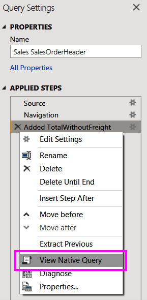
Figure 3.1 – The View Native Query option in Query Settings

You can check the native query to see how Power BI is translating your calculation to the data source's native query language to assess if it might have performance implications. The following example shows the native query for a table where a single calculation was added. The source is a SQL server and the calculation is a simple subtraction of two numerical columns:

Figure 3.2 – Native T-SQL query with a custom calculation

Tip

In DirectQuery mode, keep calculations simple to avoid generating complex queries for the underlying data source. For measures, initially limit them to sum, count, minimum, maximum, and average. Monitor the native queries generated and test responsiveness before adding more complexity, especially with CALCULATE statements.

Another point to keep in mind is that there do not need to be any physical relationships in the underlying data source to create virtual relationships in the Power BI data model. Physical relationships are created intentionally by data engineers to optimize joins between tables for common query patterns, so we want Power BI to leverage these whenever possible.

The following figure shows a simple DirectQuery model in Power BI Desktop with an arbitrary relationship created across two Dimension tables – Person and Product.

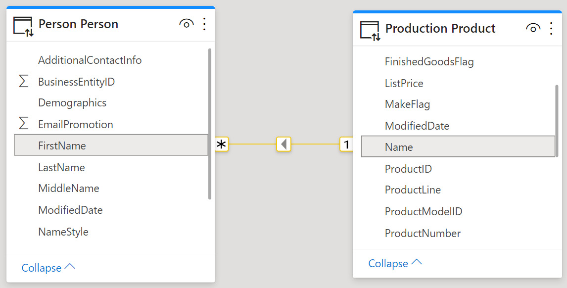
Figure 3.3 – An arbitrary relationship in DirectQuery

This trivial data model, with a single relationship, is simply for the sake of illustration. The point is that it is highly unlikely that the underlying database would have a relationship set up across these tables, and certainly not across those text columns representing the names of products and people. However, when we create such a relationship in Power BI, we are asking the data source or Power BI to perform that join on- demand. This is typically much slower as it cannot take advantage of any existing relationship optimizations at the source.

Tip

In DirectQuery mode, avoid creating relationships across tables and columns that do not have physical relationships and indexes already set up at the data source. If this cannot be avoided, consider limiting yourself to smaller tables, at least on one side of the relationship.

This was a good example of how the flexibility provided by Power BI can lead to unintended consequences if we do not fully understand the implication of our choices. There will be more of these as we progress through future chapters.

Optimizing DirectQuery relationships

Let's build further on physical relationships in the data source. There are likely to be existing Primary Key and Foreign Key columns with relationships, constraints, and indexes defined at the data source. Figure 3.4 provides a simple example from a retail sales scenario, where a territory lookup table is related to a sales order table. The TerritoryID column in each table is used for the join:

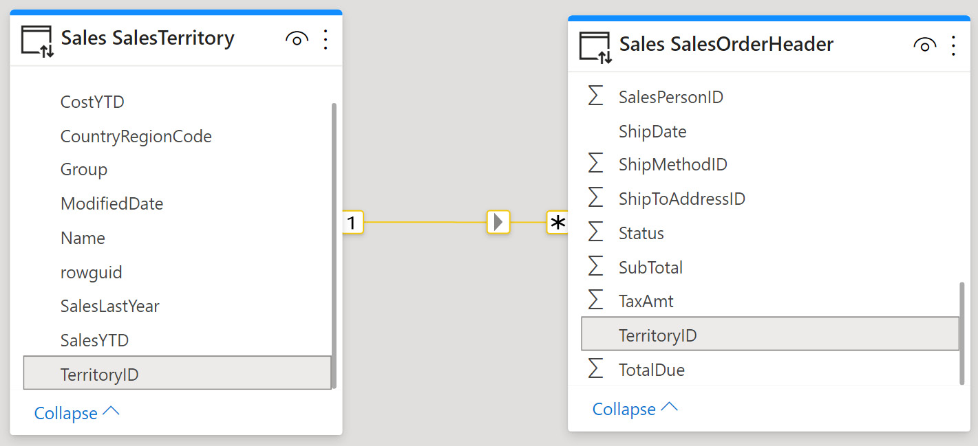
Figure 3.4 – Typical relationship to a lookup table on a numerical identifier

In cases like this, referential integrity may be enforced at the source. This means that the SalesTerritory table can be considered the master list of territories and that every entry in the SalesOrderHeader table must have a corresponding TerritoryID. This implies that there cannot be null/empty values for TerritoryID in either table. This is a good practice enforced in many database systems, which is important for Power BI because a DirectQuery dataset can issue more efficient queries to the remote data source if you can assume referential integrity.

In database terms, having referential integrity means Power BI can use an INNER JOIN instead of an OUTER JOIN when pulling data across more than one table. Referential integrity means a more efficient INNER JOIN can be used with a safe assumption that no rows from either table will be excluded due to a failure to match keys. You need to instruct Power BI to do this in the data model for each relevant relationship. The following figure shows where to do this in the relationship editor in Power BI Desktop for the sales example we discussed earlier:

Figure 3.5 – Setting referential integrity for a DirectQuery relationship

Another convenience provided by Power BI is the ability to define calculated columns, which does work for DirectQuery tables. Power BI supports building relationships using a single column from each table. However, occasionally when data modeling it may be necessary to use a combination of columns to uniquely identify some entities. A simple modeling technique to address this is to introduce a calculated column to concatenate the relevant columns into a unique key. This key column is then used to build relationships in the Power BI model. Relationships across calculated columns are not as efficient as those across physical columns. This is especially true for DirectQuery.

Tip

In DirectQuery mode, avoid creating relationships using calculated columns. This join may not be pushed down to the data source and may require additional processing in Power BI. When possible, use COMBINEVALUES() to create concatenated columns because it is specifically optimized for DirectQuery relationships.

Other ways of pushing this column calculation to the data source are to add a computed column or materialized view.

Two more aspects of relationships to consider are Cardinality and Cross filter direction (as seen in Figure 3.5). A cardinality setting of Many-to-many will disable the referential integrity setting and might result in less efficient queries if the data does in fact support a One-to-many relationship instead. Similarly, having cross filter direction set to Both (sometimes called a bi-directional relationship) could result in additional queries to the data source. This is because more tables are affected by minor report actions like slicer changes, as the filter effect needs to be cascaded across relationships in more tables. Consider whether a bi-directional relationship is necessary to support your business scenario.

Tip

Bi-directional relationships are sometimes used to have slicer values in a report update as the filter state of the report changes. Consider using a measure filter on the slicer visual to achieve the same effect. Continuing with our sales scenario as an example, this technique could be used to only show values in a product slicer if the product did have some sales.

The final piece of advice on relationships in DirectQuery concerns the Globally Unique Identifier (GUID) or slightly differently defined Universally Unique Identifier (UUID). These are represented by 32 hexadecimal characters and hyphens. An example of a GUID is 123e4567-e89b-12d3-a456-426614174000. They can be used to uniquely identify a record in a data store and are often found in Microsoft products and services.

Tip

Avoid creating logical relationships on GUID columns in DirectQuery. Power BI does not natively support this data type and needs to convert when joining. Consider adding a materialized text column or integer surrogate key in the data store instead and use those to define the relationship.

In the next section, we will look at configuration and data source optimization that can benefit DirectQuery.

Configuring for faster DirectQuery

There are a few settings that can be adjusted in Power BI to speed up DirectQuery datasets. We will explore these next.

Power BI Desktop settings

In the Power BI Desktop options, there is a section called Published dataset settings (as shown in Figure 3.6). The highlighted area shows the setting that controls how many connections per data source can be made in parallel. The default is 10. This means no matter how many visuals are in a report, or how many users are accessing the report in parallel, only 10 connections at a time will be made.

If the data source can handle more parallelism, it is recommended to increase this value before publishing the dataset to the Power BI service. However, with very busy data sources, you may find overall performance can improve by reducing the value instead. This is because too many parallel queries can overwhelm the source and result in a longer total execution time. A lower value means some queries will have to wait and be issued a little later, giving the data source some breathing room.

Important Note

Power BI Desktop will allow you to enter large numbers for the maximum connections setting. However, there are hard limits defined in the Power BI service that can differ depending on whether you are using a Premium capacity and what size your capacity is. These limits can change and are not publicly documented, so it is recommended to contact Microsoft Support to learn more for your scenario.

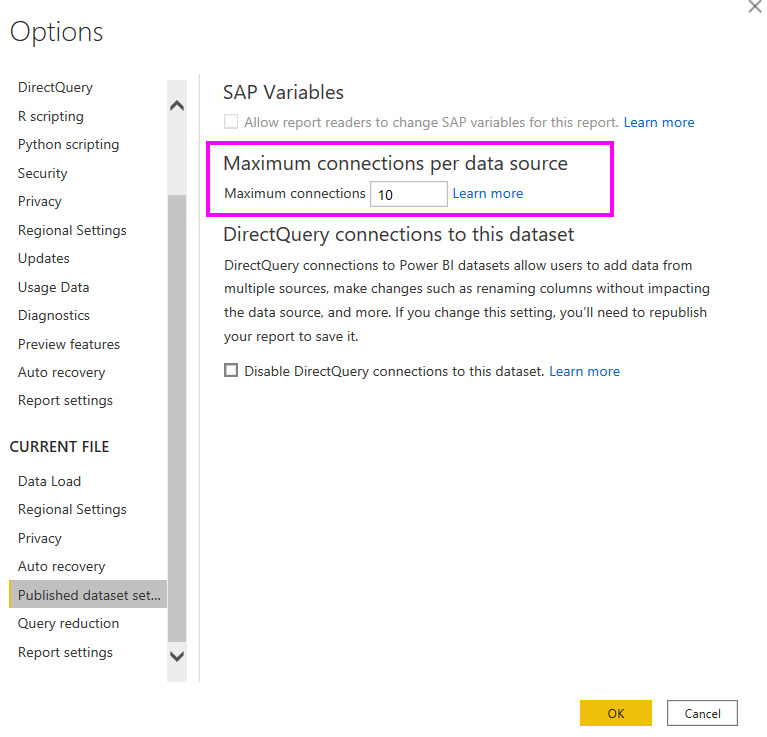
Figure 3.6 – Maximum connections per data source setting

Another useful section of Power BI Desktop options that can benefit DirectQuery is Query reduction (as shown in Figure 3.7). The figure reflects the default setting, which means that Power BI will issue queries to update visuals for every filter or slicer change a user makes in a report. This keeps the experience highly interactive but can have undesired effects with DirectQuery sources that are busy or not optimized, and with reports that have complex underlying queries. This is because the data source may not even have finished processing queries for the first filter or slicer change when the user makes further changes, which issues even more queries.

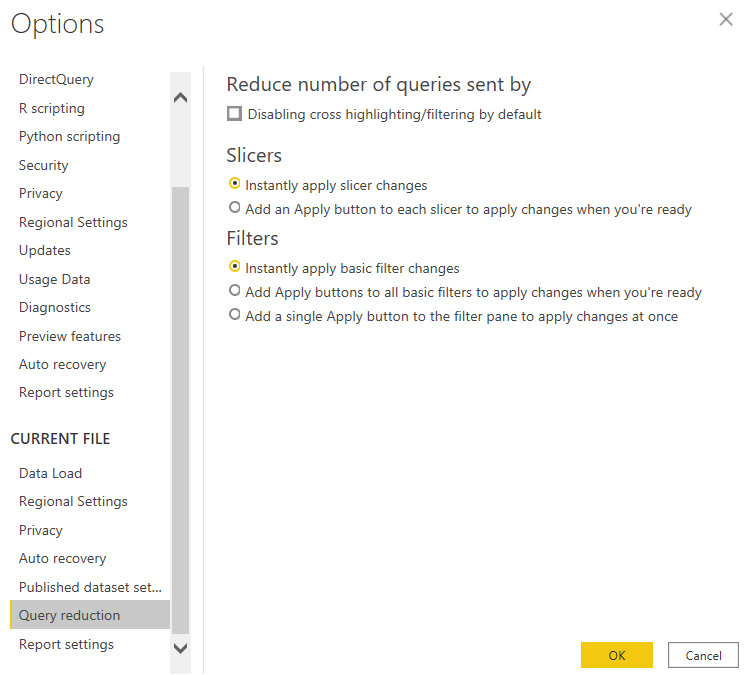
Figure 3.7 – Query reduction settings

The query reduction settings allow you to add Apply buttons for slicers and filters. This allows the user to make multiple selections before applying changes, so only a single set of queries will be sent. The report snippet in Figure 3.8 shows a single slicer and the filter pane of a report after the query reduction settings have been applied:

Figure 3.8 – Apply buttons added to slicers and filters

Next, let's look at how you can optimize the external data source to perform better in DirectQuery scenarios.

Optimizing external data sources

We have learned that DirectQuery datasets can perform slower than Import datasets because the external source might not be designed to handle workloads from Business Intelligence tools.

Regardless of what technology is powering the external data source, there are some common practices that apply to many storage systems that you should consider implementing to speed up queries for Power BI. These are as follows:

• Indexes: An index provides a database with an easy way to find specific records for operations such as filtering and joining. Consider implementing indexes on columns that you use for Power BI relationships or that are often used in report filters or slicers to limit data.
• Column storage technology: Modern data storage platforms allow you to define special indexes that use column storage instead of typical row-storage principles. This can speed up aggregate queries in Power BI reports. Try to define the index using columns that are often retrieved together for summaries in reports.
• Materialized views: A materialized view is essentially a query whose results are pre-computed and physically stored like a regular table of data. Whenever the base data changes, the materialized view is updated to reflect the current state. You can move transformations to a materialized view in the data source instead of defining them in Power BI. The source will have the results ready for Power BI to consume. This works well with data that does not change very frequently. Be aware that too many materialized views can have a performance impact on the source, as it must continually keep them up to date. Over-indexing can start reducing performance gains.
• In-memory databases: One reason Import datasets can perform very well is that they keep all data in memory instead of slower disk storage. The DirectQuery source system may have its own in-memory capabilities that could be leveraged for Power BI.
• Read-only replicas: Consider creating a read-only replica of your source system dedicated to Power BI reports. This can be optimized for Power BI traffic independently of the original data source. It can even be synchronized periodically if a real-time replica is not necessary, which can improve performance further.
• Scaling up/out: You may be able to increase the power of the source system by giving it more computing and memory resources and distributing the load across multiple servers or nodes to better handle complex parallel queries. The latter is a common pattern in Big Data systems.
• Maintaining Database Statistics: Some database systems use internal statistics to help the internal query optimizer pick the best query plan. These statistics need to be maintained regularly to ensure the optimizer is not making decisions based on incorrect cardinality and row counts.

You will need to understand what queries Power BI is sending to the external data source before you can decide what optimizations will provide the best return on investment. In Chapter 4, Analyzing Logs and Metrics, and Chapter 5, Desktop Performance Analyzer, you will learn how to capture these queries from Power BI. You can also use query logging or tracing in the external source to do this, which is more typical in production scenarios where reports are published to the Power BI service.

Let's now review the key learnings for DirectQuery datasets before we move on to discuss the sources of performance metrics available in Power BI.

Summary

In this chapter, we defined basic data modeling as a process where you choose which data attributes are grouped into entities and how those entities are related to one another. We learned that for DirectQuery, transformations in Power Query should be kept simple to avoid generating overly complex query statements for the external source system. We also learned how to use the native query viewing feature in Power Query to see the exact query Power BI will use. We saw how transformations can also be translated to native query language.

We learned that Power BI is flexible enough to allow you to define your own relationships across DirectQuery tables not necessarily matching those already in the data source. This must be used with care and some planning. It is better to leverage relationships and referential integrity that are already defined in the external data source where possible as these are likely already optimized for joining and filtering. We also explored relationship settings and their implications for DirectQuery.

Next, we explored settings in Power BI Desktop that can be used to control the level of parallelism at the data source and report level. We concluded by learning about the ways in which many widely available data platforms can be optimized and scaled to improve the performance of DirectQuery models. These external optimizations may require collaboration with other administration teams to implement options, run tests, and choose the ones that make the most sense for Power BI.

In the next chapter, we will highlight different sources of performance metrics available in Power BI, what data they make available to you and which areas of performance tuning they can help you with.