Chapter 2: Exploring Power BI Architecture and Configuration

In the previous chapter, we established guidelines for setting reasonable performance targets and gained an understanding of the major solution areas and Power BI components that should be considered for holistic performance management.

In this chapter, you will dig deeper into specific architectural choices, learning how and why these decisions affect your solution's performance. You will learn to consider broad requirements and make an informed decision to design a solution that meets the needs of different stakeholders. Ultimately, this chapter will help you choose the best components to host your data within Power BI. We will focus mainly on the efficient movement of data from the source system to end users by improving data throughput and minimizing latency.

We will begin by looking at data storage modes in Power BI and how the data reaches the Power BI dataset. We will cover how to best deploy Power BI gateways, which are commonly used to connect to external data sources. These aspects are important because users often demand up-to-date data, or historical data, and can number in the thousands of parallel users in very large deployments.

This chapter is broken down into the following sections:

• Understanding data connectivity and storage modes
• Reaching on-premises data through gateways
• General architectural guidance

Understanding data connectivity and storage modes

Choosing a data connectivity and storage mode is usually the first major decision that must be made when setting up a brand-new solution in Power BI. This means choosing between Import and DirectQuery, which we introduced in the previous chapter. Within Power BI Desktop, you need to make this decision as soon as you connect to a data source and before you can see a preview of the data to begin modeling.

Important Note

Not every data connector in Power BI supports DirectQuery mode. Some only offer Import mode. You should be aware of this because it means you may need to use other techniques to maintain data freshness when a dataset combines different data sources.

Figure 2.1 shows a SQL Server data source connection offering both Import and DirectQuery modes:

Figure 2.1 – Data connectivity options for a SQL Server source

Excel workbooks can only be configured as Import mode. Figure 2.2 demonstrates this, where we can only see a Load button without any choices for data connectivity mode. This implies that it is Import mode.

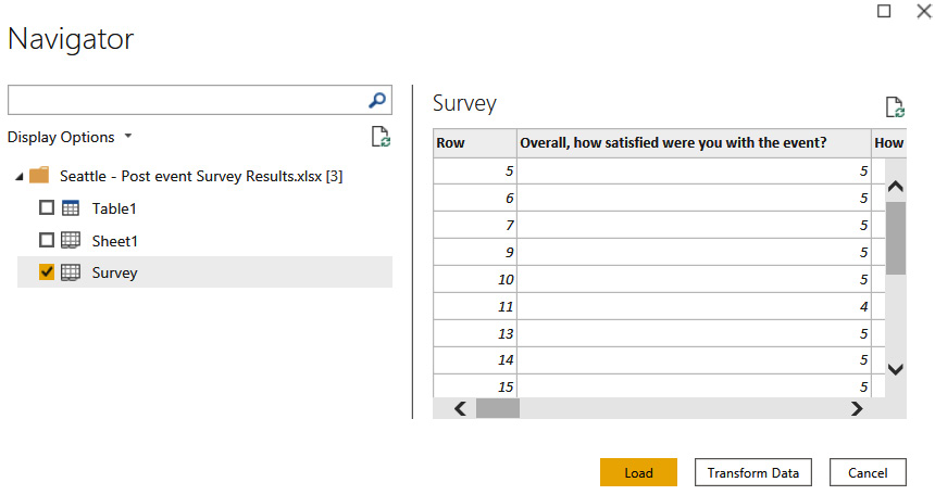
Figure 2.2 – Data connection for Excel showing no Import/DirectQuery choice

Choosing between Import and DirectQuery mode

Import data connectivity mode is the default choice in Power BI because it is the fastest, sometimes by orders of magnitude. Import mode tables store the data in a Power BI dataset, which is effectively an in-memory cache. A necessary first step for Import mode tables is to copy that source data into the Power BI Service, usually locally within the same geographical Power BI region that is processing reports. This is known as the home region. A DirectQuery source is not necessarily close to the Power BI home region. If it is not in the home region, the data needs to travel further to reach the Power BI report. Also, depending on how the data model is set up in DirectQuery, the Analysis Services engine may need to perform expensive processing on the data for each report interaction or analytical query.

Therefore, from a purely performance-oriented standpoint, we recommend Import mode over DirectQuery as it offers the best interactive experience. There are exceptions to this general rule, however, which we will explore in later sections.

The other reason why Import models are much faster is that they use Power BI's proprietary xVelocity storage also known as VertiPaq. xVelocity is a column-based storage engine, as opposed to row-based storage typically found in many database products. Column-based storage came about to deal with how badly row-based transactional databases handled queries from typical business reporting tools. They do many aggregations, potentially over large volumes of data while also offering detailed data exploration capability.

Row-based data storage engines physically store information in groups of rows. This works well when used by transactional systems because they frequently read and write individual or small groups of rows. They end up using most or all columns in the underlying table and were traditionally optimized to save and retrieve whole rows of data. Consider a sales management system where a new order is entered into a system – this would require writing a few complete rows in the database. Now consider the same system being used to view an invoice on screen – this would read a few rows from various tables and likely use most of the columns in the underlying tables.

Now, let's consider typical reporting and analytical queries for the same sales management system. Business staff would most often be looking at aggregate data such as sales and revenue figures by month, broken down into various categories or being filtered by them. These queries need to look at large volumes of data to work out the aggregates, and they often ignore many columns available in the underlying tables. This access pattern led to column-based storage engines, which store columns physically instead of rows. They are optimized to perform aggregates and filtering on columns of data without having to retrieve entire rows with many redundant columns that do not need to be displayed. They also recognize that there is often significant repetition within a column of data; that is, the same values can be found many times. This fact can be leveraged to apply compression to the columns by not storing the same physical values many times. The xVelocity engine in Power BI does exactly this – it applies different compression algorithms to columns depending on their data type. This concept of reducing repetition to reduce data size is not new and is the same technique you end up using when you compress or zip files on a computer to make them smaller.

The following diagram shows a simplified view of a table of data represented as rows or columns. The bold sections demonstrate how the data will be physically grouped. In column storage, repeating values such as customer ID 16 can be compressed to save space.

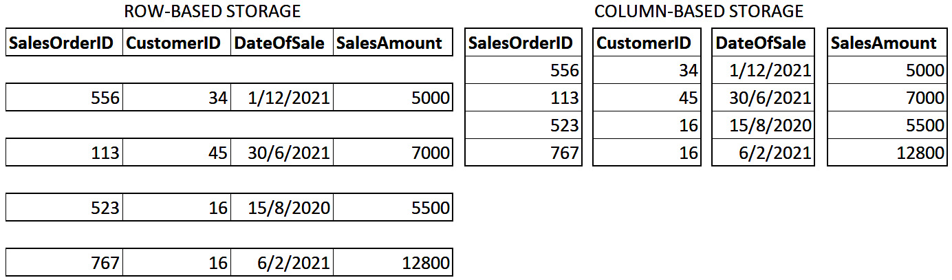
Figure 2.3 – Comparison of row and column storage

In summary, xVelocity's column-based compression technology gives you the best speed by bringing the data close to reports and squeezing that data down to significantly less than the original size. In Chapter 10, Data Modeling and Row-Level Security, you will learn how to optimize import models. Keeping Import models as small as possible will help you avoid hitting system limits such as the per-workspace storage limit of 10 GB in Shared capacity.

Important Note

A good rule of thumb is that Import mode tables using xVelocity are about 5x-10x smaller. For example, 1 GB of raw source data could fit into a 100 MB-200 MB Power BI dataset. It is often possible to get even higher compression depending on the cardinality of your data.

Next, we will look at legitimate reasons to avoid Import mode.

When DirectQuery is more appropriate

While Import mode offers us great benefits in terms of dataset size and query speed, there are some good reasons to choose DirectQuery instead. Sometimes, you will not have a choice and requirements will dictate the use of DirectQuery.

The main difference with DirectQuery, as the name implies, is that queries against the Power BI dataset will send queries to the source system. The advantage of this configuration is that you get the latest information all the time. Data is not copied into the Power BI dataset, which contains only metadata such as column names and relationships. This means that there is no need to configure data refresh or to wait for refreshes to complete before you can work with the latest data. Thus, it is typical to find DirectQuery datasets ranging in size from a few kilobytes to about 2 MB.

Important Note

Import versus DirectQuery is a trade-off. Import gives you the best query performance while needing data refresh management and potentially not having the latest data available. DirectQuery can get you the latest data and allow you to have data sizes beyond Power BI's dataset size limits. DirectQuery sacrifices some query speed and can add optimization work to the source system.

Here are the major reasons why you would use DirectQuery mode:

• Extremely large data volumes: A dataset published to a workspace on a Power BI Premium capacity can be up to 10 GB in size. A dataset published to a workspace on Shared capacity can be up to 1 GB in size. These sizes refer to the Power BI Desktop file (.pbix) that is published to the Power BI service, though in Premium datasets can grow far beyond the 10GB publication limit. If you have significantly more data, it may be impractical or simply impossible to move it into Power BI and refresh it regularly. DirectQuery does have a 1 million row limit per query, though this should not be a cause for concern as there should not be any practical use for so much unaggregated data in a report.
• Real-time access to source data: If business requirements require real-time results from the data source for every query, the only obvious choice is DirectQuery.
• Existing data platform investments: Some organizations may already have significant investments in a data warehouse or data marts typically stored in a central database. These already contain clean data, modeled in a form that is directly consumable by analysts and business users, and act as a single source of truth. These data sources are likely to be accessed by different reporting tools and a consistent, up-to-date view is expected across these tools. You may want to use DirectQuery here to fit into this central source of truth model and not have older copies in a Power BI dataset.
• Regulatory or compliance requirements: Laws or company policies that restrict where data can be stored and processed may require source data to remain within a specific geographical or political boundary. This is often referred to as data sovereignty. If you cannot move the data into Power BI because it would break compliance, you may be forced to use DirectQuery mode.

Like Import, DirectQuery mode can also benefit from specific optimization. This will be covered in detail in Chapter 3, DirectQuery Optimization.

Now that we have investigated both Import and DirectQuery modes and you understand the trade-offs, we recommend bearing the following considerations in mind when choosing between them:

• How much source data do you have and at what rate will it grow?
• How compressible is your source data?
• Is Premium capacity an option that allows larger Import datasets to be hosted?
• Will a blended architecture suffice? See the following section on Composite models.

Composite models

Power BI does not limit you to using only Import or DirectQuery in a single dataset or .pbix file. It is possible to combine one or more Import mode tables with one or more DirectQuery tables in a composite model. In a composite model, the Import and DirectQuery tables would be optimized the same way you would in a strictly Import-only or strictly DirectQuery-only model. However, combined with the Aggregations feature, composite models allow you to strike a balance between report performance, data freshness, dataset size, and dataset refresh time. You will learn how to leverage aggregations in Chapter 10, Data Modeling and Row-Level Security.

LiveConnect mode

In LiveConnect mode, the report will issue queries on demand to an external Analysis Services dataset. In this way, it is like DirectQuery in that the Power BI report does not store any data in its local dataset. However, the distinction is that LiveConnect mode is only available for Analysis Services. No data modeling can be performed, and no DAX expressions can be added. The Power BI report will issue native DAX queries to the external dataset. LiveConnect mode is used in the following scenarios:

• Creating reports from a dataset available in a Power BI workspace from Power BI Desktop or Power BI Web.
• Your organization has invested in Azure Analysis Services or SQL Server Analysis Services and this is the primary central data source for Power BI reports. The top reasons for choosing this are as follows:

a) You need a high level of control around partitions, data refresh timings, scale-out, and query/refresh workload splitting.

b) Integration with CI/CD or similar automation pipelines.

c) Granular Analysis Services auditing and diagnostics are required.

d) The initial size of the dataset cannot fit into Premium capacity.

The following diagram highlights the scenarios that use LiveConnect:

Figure 2.4 – LiveConnect scenarios

Important Note

Connections to Analysis Services also support Import mode, where data is copied and only updated when a data refresh is executed. The external Analysis Services dataset may itself be in Import mode, so you should consider whether LiveConnect is indeed a better option to get the latest data. Import can be a good choice if you are simply building lookup tables for a smaller data mart or temporary analysis (for example, a list of products or customers).

The way a report connects to its data source depends on where the report is being run. A connection from Power BI Desktop from a work office may take a completely different route than a connection from the Power BI Service initiated by a person using the Power BI Web portal or mobile app. When organizations need a way to secure and control communications from Power BI to their on-premises data sources (data that is not in the cloud), they deploy Power BI Gateways. In the next section, we will discuss Power BI Gateways, their role in data architecture optimization, and specific tips on getting the most out of gateways.

Reaching on-premises data through gateways

The on-premises data gateway provides a secure communications channel between on-premises data sources and various Microsoft services, including Power BI. These cloud services include Power BI, Power Apps, Power Automate, Azure Analysis Services, and Azure Logic Apps. Gateways allow organizations to keep sensitive data sources within their network boundaries on-premises and then control how Power BI and users can access them. The gateway is available in both Enterprise and Personal versions. The remainder of this section focuses on the Enterprise version.

When a gateway is heavily loaded or undersized, this usually means slower report loading and interactive experiences for users. Worse, an overloaded gateway may be unable to make more data connections, which will result in failed queries and some empty report visuals. What can make matters worse is that users' first reaction is often to refresh the failed report, which can add even more loads to a gateway or on-premises data source.

How gateways work

Gateways are sometimes thought of as just a networking component used to channel data. While they are indeed a component of the data pipeline, gateways do more than just allow data movement. The gateway hosts Power BI's Mashup Engine and supports Import, DirectQuery, and LiveConnect connections. The gateway service must be installed on a physical or virtual server. It is important to know that the Gateway executes Power Query/M as needed, performing the processing locally on the gateway machine. In addition, the gateway compresses and then encrypts the data streams it sends to the Power BI Service. This design minimizes the amount of data sent to the cloud to reduce refresh and query duration. However, since the gateway supports such broad connectivity and performs potentially expensive processing, it is important to configure and scale gateway machines so they perform well.

Figure 2.5 – The on-premises gateway performs mashup processing locally

Good practices for gateway performance

Some general guidelines should be applied whenever gateways are deployed. We will discuss each one in the following list and provide reasons to explain how this design benefits you:

• Place gateways close to data sources: You should try to have the gateway server as physically close to the data sources as possible. Physical distance adds latency because information needs to travel further and will likely need to pass through different computers and networking infrastructure components along the way. These are referred to as hops. Each hop adds a small amount of processing delay, which can grow when networks are congested. Hence, we want to minimize both hops and physical distance. This also means having the gateway on the same network as the data source if possible, and ensuring it is a fast network. For data sources on virtual machines in the cloud, try to place them in the same region as your Power BI home region.
• Remove network throttling: Some network firewalls or proxies may be configured to throttle connections to optimize internet connectivity. This may slow down transfers through the gateway, so it is a good idea to check this with network administrators.
• Avoid running other applications or services on the gateway: This ensures that loads from other applications cannot unpredictably impact queries and users. This could be relaxed for development environments.
• Separate DirectQuery and Scheduled Refresh gateways: Import mode connections would only be used during data refresh operations and are often used more after hours when data refreshes are scheduled. Since they often contain Power Query/M data transformations, refresh operations consume both CPU and memory and may require significant amounts for complex operations on large datasets. We will learn how to optimize Power Query/M in Chapter 8, Loading, Transforming, and Refreshing Data. For DirectQuery connections, in most cases, the gateway is acting as a pass-through for query results from data sources. DirectQuery connections generally consume much less CPU and memory than Import. However, since dataset authors can perform transformations and calculations over DirectQuery data, this can consume significant CPU in bursts. Deploying multiple gateways with some dedicated to DirectQuery and others to Refresh allows you to size those gateways more predictably. This reduces the chances of unexpected slowdowns for users running reports and queries.
• Use sufficient and fast local storage: The gateway server buffers data on the disk before it sends it to the cloud. It is saved to the location %LOCALAPPDATA%MicrosoftOn-premises data gatewaySpooler.

If you are refreshing large datasets in parallel, you should ensure that you have enough local storage to temporarily host those datasets. We highly recommend using high-speed, low-latency storage options such as solid-state disks to avoid storage becoming a bottleneck.

• Understand gateway parallelism limits: The gateway will automatically configure itself to use reasonable default values for parallel operations based on the CPU cores available. We recommend monitoring the gateway and considering the sizing questions from the next section to determine whether manual configuration would benefit you. To manually configure parallelism, modify the gateway configuration file found at Program FilesOn-premises data gateway Microsoft.PowerBI.DataMovement.Pipeline.GatewayCore.dll.config.

Set the following:

MashupDisableContainerAutoConfig = true

Now you can change the following properties in the configuration file to match your workload profile and available machine resources:

Figure 2.6 – A table showing available gateway configuration settings

Sizing gateways

Most organizations start with a single gateway server and then scale up and/or out based on their real-world data needs. It is very important to follow the minimum specifications suggested by Microsoft for a production gateway. At the time of writing, Microsoft recommends a machine with at least 8 CPU cores, 8 GB RAM, and multiple gigabit network adapters. Regular monitoring is recommended to understand what load patterns the gateway experiences and which resources are under pressure. We will cover monitoring later in this chapter.

Unfortunately, there is no simple formula to apply to get gateway sizing exactly right. However, with some planning and the right tools, you can get a good idea of what your resource needs will be and when you should consider scaling out.

We have already learned that the gateway supports different connection types. The type and number of connections will largely determine resource usage on the gateway server. Therefore, you should keep the following questions in mind when planning a gateway deployment:

• How many concurrent dataset refreshes will the gateway need to support?
• How much data is going to be transferred during the refresh?
• Is the refresh performing complex transformations?
• How many users would hit a DirectQuery or LiveConnect source in parallel?
• How many visuals are in the most used DirectQuery/LiveConnect reports? Each data-driven visual will generate at least one query to the data source.
• How many reports use Automatic Page Refresh and what is the refresh frequency?

In the next section, we will look at how to monitor a gateway and gather data to inform sizing and scaling to ensure consistent performance.

Configuring gateway performance logging

The on-premises gateway has performance logging enabled by default. There are two types of logs captured – query executions and system counters. They can be disabled by changing the corresponding value property to True in the gateway configuration file. The following shows the default settings:

<setting name="DisableQueryExecutionReport" serializeAs="String">

  <value>False</value>

</setting>

<setting name=" DisableSystemCounterReport" serializeAs="String">

  <value>False</value>

</setting>

Other settings you can adjust that affect performance logging are shown here:

• ReportFilePath: This is the path where the log files are stored. This path defaults to either UsersPBIEgwServiceAppDataLocalMicrosoftOn-premises data gatewayReport or WindowsServiceProfilesPBIEgwServiceAppDataLocalMicrosoftOn-premises data gatewayReport. The path depends on the OS version. If you use a different gateway service account, you must replace this part of the path with your service account name.
• ReportFileCount: The gateway splits log files up when they reach a predetermined size. This makes it easy to parse and analyze specific time periods. This setting determines the number of log files of each kind to retain. The default value is 10. When the limit is reached, the oldest file is deleted.
• ReportFileSizeInBytes: This is the maximum size of each log file. The default value is 104,857,600 (100 MB). The time period covered in each file can differ depending on the amount of activity captured.
• QueryExecutionAggregationTimeInMinutes: Query Execution metrics are reported in aggregate. This setting determines the number of minutes for which the query execution information is aggregated. The default value is 5.
• SystemCounterAggregationTimeInMinutes: System Counters metrics are also aggregated. This setting determines the number of minutes for which the system counter is aggregated. The default value is 5.

When logging is enabled, you will start to collect information in four sets of files with the .log extension and numerical suffixes in the filename. The log file group names are provided in the following list.

• QueryExecutionReport: These logs contain detailed information on every query execution. They tell you whether the query was successful, the data source information, the type of query, how long is spent executing and data processing, how long it took to write data to disk, how much data was written, and what the average speed is of the disk operations. This information is invaluable as it can be used to work out where bottlenecks are at a query level.
• QueryStartReport: These are simpler query logs that provide the actual query text, data source information, and when the query started. You can see the exact query that was sent to data sources, which can be useful for performance troubleshooting, especially with DirectQuery data sources. You will learn how to optimize systems for DirectQuery in Chapter 3, DirectQuery Optimization.
• QueryExecutionAggregationReport: These logs contain aggregated query information in buckets of 5 minutes by default. They provide useful summary information such as the number of queries within the time window, the average/minimum/maximum query execution duration, and the average/minimum/maximum data processing duration.
• SystemCounterAggregationReport: This log contains aggregated system resource information from the gateway server. It aggregates average/minimum/maximum CPU and memory usage for the gateway machine, gateway service, and the mashup engine.

  Important Note

  You need to restart the gateway after adjusting any settings to apply the changes. It can take up to 10 minutes plus the QueryAggregationTimeInMinutes value to see log files appearing on the disk.

Parsing and modeling gateway logs

Microsoft has provided a basic Power BI report template to help you analyze gateway data. This template can be found at the following link: https://download.microsoft.com/download/D/A/1/DA1FDDB8-6DA8-4F50-B4D0-18019591E182/GatewayPerformanceMonitoring.pbit.

The template will scan your log folder and process all the files it finds that match the default naming pattern. It parses and expands complex columns, for example, JSON, and leaves you with the following data model.

Figure 2.7 – Report data model from the Microsoft Gateway Performance template

The following figure demonstrates one of the default views in the Gateway Performance template:

Figure 2.8 – Example of gateway performance visualization from the template

The Microsoft-provided template does a reasonable job of giving you visibility on some aggregate and detailed operations on the gateway. However, to extract further value from it, you will likely need to make some changes to the transformations, data model, and calculations. This could take some work to perfect, so it may be worth considering whether a pre-built option is feasible. If your organization uses Microsoft Premier or Unified Support, you may have access to Power BI performance assessments. These are run by experienced customer engineers who have enhanced templates to analyze gateway logs. Another option is to engage consultants who have a professional solution on the market. A web search for Microsoft partners who offer such a solution will help you identify and evaluate the costs and benefits.

If you choose to build on the Microsoft template yourself, do consider the following improvements:

• Automate the retrieval and storage of logs from the gateway server, for example, with PowerShell scripts.
• Build separate date and time dimensions and connect them to all the log tables so that you can build reports that can look at time-correlated activity across every log.
• Build common dimension tables for Query Status, Query Type, and Data Source from the log files and connect them to each log table. This will allow you to slice report pages using the same filter across different logs.
• Add a dimension table containing details of all your gateways, such as the environment, gateway ID, name, memory size, and CPU core count. Use the gateway ID to connect it to the fact tables log.
• Build report views that focus on trends and aggregates to highlight spikes in CPU or memory while able to distinguish between DirectQuery and Refresh queries. Further details are provided in the next section.

Next, we'll look at gateway logs.

Analyzing gateway logs

We suggest that the initial views you build on gateway logs will help you to answer high-level questions and spot problems areas quickly. Here are some important questions you should be able to answer:

• Are there any spikes in overall gateway resource usage and do the spikes recur regularly?
• When I reach high or maximum resource usage, what is the workload pattern?
• What datasets, dataflows, or reports consume the most gateway resources?
• What is the gateway throughput in terms of queries per second and bytes processed per second?
• When I see throughput drops, what operations were running in that time slice, and which contributed most from a resource perspective?
• Is the gateway performing many Refresh and DirectQuery operations in parallel? This is likely to create pressure on CPU and memory at the same time, so consider dedicated DirectQuery and Refresh gateways, spreading out Refresh operations, and scaling.
• What is the average query duration over time and what contributes to increases – gateway resource limits or growing data volume/query complexity?
• What are the slowest queries? Are they consistently slow or does the performance vary greatly? The former may suggest query or model design issues, or that optimization may be needed at the data source or even the network. The varying performance of the same queries suggests unpredictable loads on the gateway or data source are the issue.

  Tip

  Go back to the Sizing gateways section and review the high-level questions to ask when sizing the gateway. See how they connect with the detailed questions and data points we just covered. This will help you build guidance for your organization, understanding what size of gateway is needed for your workloads and data sources.

Next, we will look at when you should consider scaling and how to do so.

Scaling up gateways

It is possible to manage a gateway well but still begin to reach resource limits due to data and usage growth. Scaling up is simply adding more resources or replacing them with faster components. You know it is time to scale when your analysis shows you are hitting a memory, CPU, or disk limit and may have no more room to move in changing Refresh schedules or optimizing other layers of the solution. We will cover such optimizations in detail in subsequent chapters.

For now, let's assume that the deployed solutions are perfect, yet you are seeing performance degradation and an increase in query failures caused by excessive loads. The first choice here should be to scale up. You may choose to increase the number of CPU cores and memory independently if your analysis identified only one as the problem and you see enough headroom in the other. While CPU and memory are the common candidates for scaling up, do keep an eye on disk and network performance too. You may need to scale those up too or scale out if this is not an option.

Scaling out with multiple gateways

When you can no longer effectively scale up a single gateway machine, you should consider setting up a gateway cluster. This will allow you to load balance across more than one gateway machine. Clusters also provide high availability through redundancy in case one machine goes down for whatever reason.

To create a gateway cluster, you simply run the gateway installer on a different server. At the time of installation, you will be given the option of connecting the gateway to an existing gateway server, which acts as the primary instance. This is shown in the following screenshot:

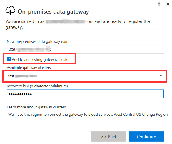
Figure 2.9 – Adding a gateway to a cluster by selecting the primary instance

All requests are routed to the primary instance of a gateway cluster. The request is routed to another gateway instance in the cluster only if the primary gateway instance is offline.

Tip

If a gateway member server goes down, you should remove it from the cluster using the Remove-OnPremisesDataGateway PowerShell command. If not, query requests may still be sent to it, which can reduce performance.

Load balancing on the gateway is random by default. You can change this to balance load based on CPU or memory thresholds. This will change the behavior so when a member is at or over the throttling limit, another member within the cluster is selected. The request will fail only if all members within the cluster are above the limits.

A gateway admin must update settings in the config file introduced earlier (the Program FilesOn-premises data gateway Microsoft.PowerBI.DataMovement.Pipeline.GatewayCore.dll.config file).

The following settings can be adjusted to control load balancing:

• CPUUtilizationPercentageThreshold: A value between 0 and 100 that sets the throttling limit for CPU. 0 means the configuration is disabled.
• MemoryUtilizationPercentageThreshold: A value between 0 and 100 that sets the throttling limit for memory. 0 means the configuration is disabled.
• ResourceUtilizationAggregationPeriodInMinutes: The time window in minutes for which CPU and memory system counters of the gateway machine are aggregated. These aggregates are compared against the thresholds defined beforehand. The default value is 5.

Now that we have a good grasp of storage modes and gateway optimization, we will consider broader factors that come into play and can slow down operations in these areas.

General architectural guidance

This section presents general architectural best practices that can help with performance.

Planning data and cache refresh schedules

A sometimes-overlooked consideration is how fresh an Import dataset's sources are. There is no point refreshing a dataset multiple times a day if it relies on an external data mart that is only refreshed nightly. This adds an unnecessary load to data sources and the Power BI service.

Look at your environment to see when refresh operations are happening and how long they are taking. If many are happening in parallel, this could slow down other operations due to intense CPU and memory usage. The effect can be larger with Power BI Premium. Consider working with dataset owners to remove unnecessary refreshes or change timings so that they do not occur altogether, but are potentially staggered instead. A data refresh in progress can require as much additional memory as the dataset itself, sometimes more if the transformations are complex or inefficient. A general rule of thumb is that a refreshing dataset consumes twice the memory.

Reduce network latency

In an earlier section, we discussed how reducing the physical distance and hops between data sources helps to reduce network latency. Here are additional considerations:

• Co-locate your data sources, gateways, and other services as much as possible, at least for production. If you relied on Azure, for example, it would be recommended to use the same Azure region as your Power BI home tenant region.
• Consider a cloud replica of on-premises data sources. This incurs some cloud costs but can significantly reduce latency for Power BI if the cloud region is far from the on-premises data center.
• If your data is in the cloud, consider performing Power BI development through remote desktop into cloud virtual machines. Those virtual machines should ideally be in the same region as the data sources.
• Use Azure ExpressRoute to have a secure, dedicated, high-speed connection from your on-premises network to the Azure Cloud.

Now that you have a good understanding of the architectural choices that affect performance in Power BI, let's summarize what we've learned before we explore the next area of performance in Power BI.

Summary

In this chapter, we saw how the two storage modes in Power BI work. Import mode datasets create a local in-memory cache of the data in Power BI. DirectQuery mode datasets pass queries through to external data sources. Generally, Import mode is the fastest because it is local to Power BI, in-memory, a column-based database, and compresses data to make working with it more efficient. However, DirectQuery mode provides a way to always have the latest data returned from the source and avoid managing data refreshes. It also allows you to access very large datasets that are far beyond the capacity available in Power BI Premium. In this way, there is a trade-off between these two modes. However, Power BI also provides composite models that blend Import and DirectQuery for very good performance gains.

You have also learned the role of on-premises gateways for enterprises to allow Power BI to connect securely with on-premises data sources. Gateways host Power BI's mashup engine, where data transformations are performed locally. These can be resource hungry, especially with hundreds or thousands of users, which could translate to many connections per second. This means gateways need to be sized, monitored, and scaled. Hence, we looked at the high-level questions that should be asked, for example, relating to a simultaneous refresh or user counts. We then looked at gateway performance logging to provide data to get the answers to these questions and inform scaling. We introduced the gateway performance monitoring template provided by Microsoft and suggested improvements for better usability. Then we learned what patterns to look for when analyzing logs and questions to help drive the correlation of data. This helps us determine when to scale up a gateway or scale out to gateway clusters and load balancing.

We then explored how to plan data refresh to prevent periods of too much parallel activity. Finally, we learned how to reduce data and network latency in other ways for development and production scenarios.

In the next chapter, we will extend the topic of storage modes further by focusing specifically on optimizing DirectQuery models. This will involve guidance for the Power BI dataset and the external data source.