Chapter 8: Loading, Transforming, and Refreshing Data

So far, we have focused a lot on performance monitoring and investigation. We have now reached the next phase of our journey into Power BI performance management. Here, we will begin looking at what actions we can take to remedy the performance issues we discovered while using the tools that were introduced in previous chapters. From here on, each chapter will look deep at a specific area of a Power BI solution and will provide performance guidance. The first of these is loading data into Power BI.

Loading new data periodically is a critical part of any analytical system, and in Power BI, this applies to Import mode datasets. Data refresh and its associated transformations can be some of the most CPU and memory-intensive operations. This can affect user activities and cause refresh failures. Large datasets that occupy a significant portion of a host's memory, and that have complex data transformations, are more prone to resource contention. Poorly designed transformations contribute to high resource usage and can result in refresh failures. They can even affect development productivity by slowing down or, in extreme cases, crashing Power BI Desktop.

In this chapter, we will learn how Power BI's Power Query transformation engine works and how to design queries with performance in mind. Additionally, we'll learn how to use the strengths of data sources and avoid pitfalls in query design with the aim of reducing CPU and memory use. This provides benefits when the datasets are still in development and when they are deployed to production.

In this chapter, we will cover the following main topics:

• General data transformation guidance
• Folding, joining, and aggregating
• Using query diagnostics
• Optimizing dataflows

Technical requirements

There are examples available for some parts of this chapter. We will call out which files to refer to. Please check out the Chapter08 folder on GitHub to get these assets: https://github.com/PacktPublishing/Microsoft-Power-BI-Performance-Best-Practices.

General data transformation guidance

Power Query allows users to build relatively complex data transformation pipelines through a point and click interface. Each step of the query is defined by a line of M script that has been autogenerated by the UI. It's quite easy to load data from multiple sources and perform a wide range of transformations in a somewhat arbitrary order. Suboptimal step ordering and configuration can use unnecessary resources and slow down the data refresh. Sometimes, the problem might not be apparent in Power BI Desktop. This is more likely when using smaller subsets of data for development, which is a common practice. Hence, it's important to apply good Power Query design practices to avoid surprises. Let's begin by looking at how Power Query uses resources.

Data refresh, parallelism, and resource usage

When you perform a data refresh for an Import mode dataset in the Power BI service, the dataset stays online. It can still be queried by published reports or even from Power BI Desktop and other client tools such as Excel. This is because a second copy of the dataset is refreshed in the background, while the original one is still online and can serve users. However, this functionality comes at a price because both copies take up memory. Furthermore, transformations that are being performed on the incoming data also use memory.

Tip

For a full refresh, you should assume that a dataset will need at least two times its size in memory to be able to refresh successfully. Those with complex or inefficient transformations might use significantly more memory. In practical terms, this means a 2 GB dataset would need at least 4 GB of memory available to refresh.

The actual work of loading and transforming data in Power BI is performed by the Power Query mashup engine. The host, as mentioned at the beginning of the chapter, refers to the machine where this mashup engine is running. This host could be Power BI Desktop, the Power BI service, a Premium capacity, or a gateway. Each table being refreshed runs in an evaluation container. In Power BI Desktop, each container is allocated 432 MB of physical memory by default. If a container requires more physical memory than this, it will use virtual memory and be paged to disk, which dramatically slows it down.

Additionally, the number of containers executing in parallel depends on the host. In Power BI Desktop, the number of containers running in parallel defaults to the number of logical cores available on the machine. This can be adjusted in the Data Load section of the Power Query settings pane. Also, you can adjust the amount of memory used by each container. These settings can be seen in the following screenshot:

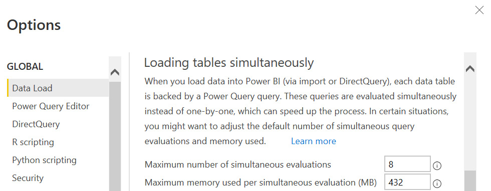
Figure 8.1 – The Power Query parallel loading settings

Some data transformations require a lot of memory for temporary data storage. If the container memory is completely used up, the operation pages to disk, which is much slower.

Tip

You can use Resource Monitor, which is built into Windows to observe the memory usage of Power Query . In the memory section, look for a process name such as Microsoft.Mashup.Container. If you see a Commit value that is much higher than the Working Set, that means paging is occurring. To avoid paging in Power BI Desktop, one option is to increase the amount of container memory. Be aware that setting this too high could use up all available memory and affect your system's responsiveness. Before increasing memory, you should optimize your query, as we will describe later.

There probably isn't much benefit in increasing the number of containers in Power BI Desktop significantly beyond the default. The default setting will assign one container per available logical core, and they will all run in parallel. Depending on the complexity of the transformations and what else is running on the development computer, this might have a reasonable load. Having too many containers could end up slowing down the overall refresh operation by trying to run too many things in parallel and creating CPU contention. Each CPU core ends up juggling multiple queries. Finally, the data source also needs to handle that many simultaneous connections. It might have its own connection limits or policies in place.

For Power BI Premium, Power BI Embedded, and Azure Analysis Services, you cannot modify the number of containers or memory settings through any UI. The limits depend on the SKU and are managed by Microsoft. However, using the XMLA endpoint, you can manually override the setting for how many tables or partitions can be processed in parallel. This is done by using the sequence command in a TMSL script. You can use a tool such as SQL Server Management Studio to connect to your dataset and execute it. The following example uses a sequence command to enable 10 parallel evaluation containers. Note that only one table is listed as an example. You can simply modify this script and specify more tables/partitions in the area indicated:

{

  "sequence":{

    "maxParallelism":10,

    "operations":[

      {

        "refresh":{

          "type":"full",

          "objects":[

            {

              "database":"ExampleDataset",

              "table":"ExampleLogs",

              "partition":"ExampleLogs202112"

            }

            

           // specify further tables and partitions here

          ]

        }

      }

    ]

  }

}

Now, let's see how to make working with queries faster in Power BI Desktop.

Improving the development experience

When working with significant data volumes, complex transformations, or slow data sources, the Power BI Desktop development environment can occasionally slow down or become non-responsive. One reason for this is that a local data cache is maintained to show you data previews for each transformation step, and Power BI tries to refresh this in the background. It can also be caused if there are many dynamic queries being driven by a parameter. When properly used, query parameters are a good Power Query design practice. However, a single parameter change can cause many previews to be updated at once, and this can slow things down and put excess load on the data source.

If you experience such issues, you can turn off Background Data in the Power Query settings, as shown in Figure 8.2. This will cause a preview to only be generated when you select a query step. The appropriate setting is shown in the following screenshot. The screenshot also shows a setting to prevent Parallel loading of tables. This is very useful in scenarios where you are running many complex queries and know for certain that the source would handle sequential queries better. Often, this is the case when using handwritten native queries for a data source with many joins, transformations, and summarizations:

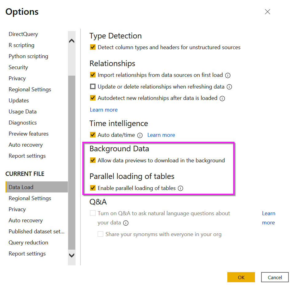
Figure 8.2 – The Data Load settings to disable complex queries

Another method for reducing the load on the source while still in development is to use a simple toggle parameter to limit the amount of data returned. The following screenshot shows how a Binary parameter, called DevelopmentFlag, appears when given possible values of 0 and 1:

Figure 8.3 – A toggle parameter showing possible values

Once the parameter is ready, you can use it in queries. In the following screenshot, we show how a conditional statement can be used in Advanced Editor to leverage this toggle. When the toggle is set to 1, Power Query only gets data prior to June 1, 2013, from the #"Filtered Rows" step. If the toggle is set to 0, it will pick up the result from the previous Fact_Transaction step instead. This is a practical example of a useful ability in Power Query to reference previous states of queries:

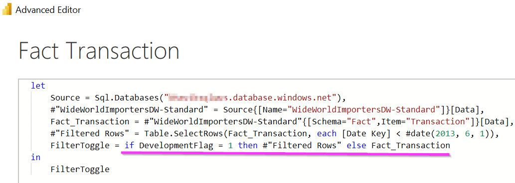
Figure 8.4 – Using the toggle parameter to reduce data

If you are using multiple data sources and are using values from one source to control the queries of another, you can experience lower performance with the default privacy settings. This is because Power Query prevents any leakage of data from one source to another for security reasons. For example, if you use values from one database to filter data from another, the values you pass could be logged and viewed by unintended people. Power Query prevents this leakage by pulling all the data locally and then applying the filter. This takes longer because Power Query must wait to read all the data. Also, it can't take advantage of any optimizations at the source through indexing and other techniques.

If you are comfortable with the risks associated with data leakage, you can disable the Privacy Levels setting, as shown in the following screenshot. This shows a global setting. However, note that you can also set this individually for each .pbix file much lower down in the settings (not shown):

Figure 8.5 – Ignoring the privacy level settings can improve performance

Another helpful Power Query technique is using the reference feature to use one query to start a new query. This is useful when you need to split a data stream into multiple formats or filter and transform subsets differently. A common mistake is to leave this referenced table available in the data model even though it is never directly used in reports. Even if you hide it from users, it will still be loaded and occupy memory. In such cases, it's better to turn off the Enable Load option, which can be found by right-clicking on the query. Disabling the load will only temporarily keep the table during refresh and reduce the dataset's memory footprint. In the following screenshot example, the CSVs source contains two different groups of records, Student and Course. Once these groups are separated out into their own tables, the starting table does not need to be loaded:

Figure 8.6 – How to turn off loading intermediate tables

A technique that can help you with complex transformations that happen in Power Query is the use of buffer functions. Power Query has two flavors that are relevant to us, Table.Buffer() and List.Buffer(). You can wrap these around a Table object or a List object in Power Query to force it to be loaded into memory and kept there for later use instead of streaming it in small batches. This can be useful when dealing with certain transformations, such as extracting entire tables from single columns (for example, JSON documents) or pivoting/unpivoting dynamically over large numbers of unique values, especially with multiple levels of nested functions. A good time to consider buffer functions is when you get refresh failures indicating that the resources were exhausted.

A final tip is to consider whether you really need the automatic date/time feature in Power BI. When enabled, it will create a hidden internal date table associated with every date or date/time field found in the dataset. This can take up significant space if you have a wide range of dates and many date fields. A better practice is to use your own date dimension tables that are connected to only the meaningful dates that need aggregations to month and year:

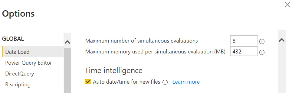
Figure 8.7 – Time intelligence in the Power Query settings

Next, we'll look at ways to leverage the strengths of large data stores to offload work from Power Query and reduce refresh times.

Folding, joining, and aggregating

While Power Query has its own capable data shaping engine, it can push down certain transformations to data sources in their native query language. This is known as Query Folding, and formally, it means that the mashup engine can translate your transformation steps into a single SELECT statement that is sent to the data source.

Tip

Query Folding is an important concept as it can provide huge performance benefits. Folding minimizes the amount of data being returned to Power BI, and it can make a huge difference for refresh times or DirectQuery performance with large data volumes of many millions of rows.

There is a bit of knowledge and trial and error required to get the best folding setup. You know a query step is folded when you can right-click on it and see the View Native Query option enabled, as shown in the following screenshot:

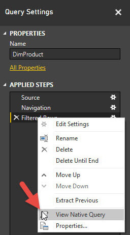
Figure 8.8 – View Native Query indicates that folding has occurred

Ideally, you will want to see the last step of your query that allows you to view the native query because this means the entire query has been folded. This seems straightforward enough, but it's important to understand which operations can be folded and which can break a chain of otherwise foldable operations. This depends on the individual data source, and the documentation is not comprehensive. Not every source supports viewing a native query; one example is Odata, which is a standard for building and consuming REST APIs. You can use Query Diagnostics in such cases to learn more about what each step is doing. We will cover Query Diagnostics in the next section.

The following list of operations are typically foldable:

• Filtering rows, with static values or Power Query parameters
• Grouping and summarizing
• Pivoting and unpivoting
• Simple calculations such as arithmetic or string concatenation that translate directly to the data source
• Removing columns
• Renaming or aliasing columns
• Joining tables on a common attribute
• The non-fuzzy merging of queries based on the same source
• Appending queries based on the same source

The following list of operations are typically not foldable:

• Changing a column data type
• Adding index columns
• Merging queries based on different sources
• Appending queries based on different sources
• Adding custom columns with complex logic that have no direct equivalent in the data source

  Tip

  Perform all foldable transformations at the beginning of your query to ensure they all get pushed down to the data source. Once you insert a step that cannot be folded, all subsequent steps will occur locally in Power Query, regardless of whether they can be folded. Use the technique described in Figure 8.7 to walk through your steps in sequence, and reorder them if necessary.

Specifically, you should look out for any group, sort, or merge operations in Power Query that have not been folded. These operations require whole tables to be loaded into Power Query, and this could take a long time with large datasets and can lead to memory pressure. If a group operation cannot be pushed down, but you know the source is already sorted on the grouping column, you can improve performance by using an additional parameter to the Table.Group() function, called GroupKind.Local. This will make Power Query more efficient, as it will know a group is complete when the value changes in the next row that is processed. It can do this because it assumes the values are contiguous.

Tip

If you are fluent in the native language of the data source and are comfortable writing your own query, you can use a custom query instead of letting Power Query generate one for you. This can be a last resort to ensure that everything possible has been pushed down. It is particularly useful when you know the source data characteristics such as frequency and distribution and can use source-specific capabilities such as query hints to improve speed. Complex joins and aggregations might not be completely pushed down to the source and might benefit from being implemented within a custom query.

Leveraging incremental refresh

For data sources that support being pushed down, Power Query supports Incremental Refresh. This is a useful design pattern to consider for optimizing data refresh operations. By default, Power BI requires a full load of all tables when a dataset is using Import mode. This means all of the existing data in the table is discarded before the refresh operation. This ensures that the latest data is loaded into Power BI. However, often, this results in unchanged historical data being loaded into the dataset each time it is refreshed. If you know that you have source data that is only ever appended and historical records are never modified, you can configure individual tables in a Power BI dataset to use incremental refresh to load only the most recent data. The following steps should be followed in sequence to enable incremental refresh:

1. Before you can use the incremental refresh feature, you must add two date/time parameters, called RangeStart and RangeEnd, to control the start and end of the refresh period. The setup of the parameters is shown in the following screenshot:

Figure 8.9 – The date/time parameters required for incremental refresh

2. Next, you must use these parameters as dynamic filters to control the amount of data returned by your query. An example of this configuration is shown in the following screenshot, where the Invoice Date key column is used for filtering:

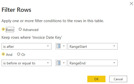
Figure 8.10 – Filter configuration to support parameterized date ranges in a query

3. Once you have a query configured to use the date range parameters, you can enable incremental refresh. You simply right-click on the table name in Power BI Desktop and select the Incremental refresh option. The following screenshot shows how the UI allowed us to select 6 months of historical data to retain, along with 1 day of new data upon each refresh, for a table called Fact Sale:

Figure 8.11 – Incremental refresh configured within a table

There are two options available in the incremental refresh setup dialog that enable you to have more control:

• Detect data changes: This will allow you to choose a timestamp column in the source database that represents the last modified date of the record. If this is available in the source, it can further improve performance by allowing Power BI to only select changed rows within the refresh period.
• Only refresh complete day: This will ensure that only the most recent complete day of data will be refreshed. This is required to ensure the accuracy of some business metrics. For example, calculating daily average users for a web application would not be accurate if considering incomplete days. In practical terms, let's suppose you schedule a data refresh at 2 a.m. daily because it will have the lowest impact on the source system. Enabling this setting will instruct Power Query to only collect data from before midnight.

Next, we will see how the built-in query diagnostics can help us to spot and resolve performance issues.

Using query diagnostics

In Power BI Desktop, you can enable query diagnostics to get a detailed understanding of what each step of your query is doing. Even with seemingly simple queries that have few transformations, if performance is bad, you will need to know which part is slowing you down so that you can concentrate your optimization efforts. Diagnostics needs to be enabled in the Power Query settings, as shown in the following screenshot. You might not need all the traces that are shown in the following screenshot. At a minimum, enable the Aggregated diagnostics level and Performance counters:

Figure 8.12 – Query Diagnostics enabled in the Power Query settings

There are up to four types of logs that are available:

• Aggregated: This is a summary view that aggregates multiple related operations into a single log entry. The exclusive durations are summed per entry.
• Detailed: This is a verbose view with no aggregation. It is recommended for complex issues or where the summary log doesn't provide enough to determine a root cause.
• Performance counters: Every half second, Power Query takes a snapshot of the current memory use, CPU utilization, and throughout. This might be negligible for queries that are fast or push all the work to the data source.
• Data privacy partitions: This helps you to identify the logical partitions that are used internally for data privacy.

Next, we will learn how to collect the traces and explore the information contained within them.

Collecting Power Query diagnostics

Diagnostic traces are not automatically collected after the settings, as shown in Figure 8.13, have been enabled. To save trace data to disk, you need to start diagnostics from the Tools menu of the Power Query Editor screen, as shown in the following screenshot:

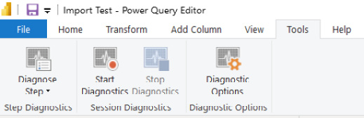
Figure 8.13 – The Power Query diagnostic controls

Select the Start Diagnostics button to enable data collection. From this point on, any query or refresh operations will be logged to disk. You can perform as many operations as you want, but nothing will be visible until you use the Stop Diagnostics button. After stopping the diagnostics, the logs are automatically added to the query editor, as shown in the following screenshot:

Figure 8.14 – The query logs are automatically loaded

You can only collect traces from the Query Editor UI. It will capture any activity, even loading previews and working on a single query step. Additionally, you can capture activity from the Report view, which is great for tracing a full table or dataset refresh. The choice you make will depend on the scenario you are trying to debug. You can select a single query step and use the Diagnose Step button to run a single step, which will create a dedicated trace file that is named after the step.

Tip

Query logs can become quite large and might become difficult to work with. The Power Query Editor UI performs background operations and caching to improve the user experience, so all steps might not be properly represented. We recommend that you only capture diagnostics for the operations or tables you are trying to debug to simplify the analysis. Start diagnostics, perform the action you want to investigate, then stop diagnostics immediately after and analyze the files.

Analyzing the Power Query logs

The Power Query log files have different schemas that might change over time. We recommend that you check out the online documentation to understand what each field means. It can be found at https://docs.microsoft.com/power-query/querydiagnostics.

We are mostly interested in the Exclusive Duration field found in the aggregate and detailed logs. This tells you how long an operation took in seconds, and it helps us to find the slowest items. The Microsoft documentation describes how you can slice the log data by the step name or ID. This is an easy way to find the slowest element, but it doesn't help you to understand which operation dependencies exist. The logs contain a hierarchical parent-child structure with arbitrary depth depending on your operation complexity. To make it easier to analyze this, we provide a Power Query function that can be used to flatten the logs into an explicit hierarchy that is easier to analyze using the decomposition tree visual. Please see the ParsePQLog.txt example file. This function is adapted from a blog post that was originally published by Chris Webb: https://blog.crossjoin.co.uk/2020/02/03/visualising-power-query-diagnostics-data-in-a-power-bi-decomposition-tree/.

We have provided examples of how the parsed data can be visualized. The following screenshot is a snippet of the Query Diagnostics.pbix example file and shows how a decomposition tree is used to explore the most expensive operation group and its children. From the tooltip, we can see that the Level 2 step took about 29 seconds and loaded over 220,000 rows. Additionally, we can see the exact SQL statement sent to the data source to confirm that folding occurred:

Figure 8.15 – A hierarchical view of a query log after flattening

Next, we will look at an example where the same query logic is performed in two different ways, that is, by only changing a data source. We'll see how this affects folding and how to investigate the impact on performance.

In this scenario, we have a data warehouse and want to create a wide de-normalized table as a quick stopgap for an analyst. We need to take a sales fact table and enrich it with qualitative data from four dimensions, such as customer and stock. The data is all in SQL Server. For the sake of this example, these tables are loaded individually into Power BI Desktop, as shown in the following screenshot. We dumped the database-hosted fact table inside a .CSV file and named it Fact Sale_disk to provide an alternative data source to perform the comparison:

Figure 8.16 – The starting tables loaded into the dataset

We perform a merge from the fact to the dimensions, expanding the columns we need after each merge. We expect this version to be folded. Additionally, we create a second version that uses the file as a source for the fact table. We expect the disk version to not be folded because the joins and filters are applied directly to the CSV on disk. The difference between these is shown in the comparison of query steps that follow. Note how FlattenedForAnalyst_NotFolded has the View Native Query option disabled, which confirms this difference:

Figure 8.17 – A comparison of the same query logic using different sources

In the following screenshot, we compare the high-level activities and durations of these two refresh operations. We can clearly see that the pure database method was significantly faster – about 10 seconds compared to about 34 seconds for the mixed database and file method. This should not be a surprise when we think about how the mashup engine works. For the pure database method, all logic was folded and sent to the data source as a single query. However, when using the fact table from the file and dimensions from the database, Power Query needs to execute queries to fetch the dimension data so that it can perform the join locally. This explains why we see significantly more activities:

Figure 8.18 – A shorter duration and fewer operations with the folded query

Now we have gained useful fundamental knowledge and analytical methods to help identify slow operations in Power Query. Next, we will explore performance tuning for dataflows.

Optimizing dataflows

A Power BI Dataflow is a type of artifact contained within a Power BI workspace. A dataflow contains Power Query data transformation logic, which is also defined in the M query language that we introduced earlier. The dataflow contains the definition of one or more tables produced by those data transformations. Once it has been successfully refreshed, the dataflow also contains a copy of the transformed data stored in Azure Data Lake.

A dataflow might seem very similar to the query objects you define in Power BI Desktop, and this is true. However, there are some important differences, as noted in the following points:

• A dataflow can only be created online through the Power BI web application via Power Query Online.
• A dataflow is a standalone artifact that can exist independently. It is not bundled or published with a dataset, but dataset items can use the dataflow as a standard data source.
• There are some UI and functionality differences between Power Query in Power BI Desktop compared to Power Query Online.
• A dataflow can be used by datasets or even other dataflows to centralize transformation logic.

The last point in the preceding bullet list is important since it describes a key reason that dataflows exist in the first place. They are designed to promote data reuse while avoiding duplicated data transformation operations and redundant processing. Let's explore this using a practical example. Let's suppose an organization encourages self-service report development so that business users can get insights quickly. They realize that many different people are trying to access a list of customers with properties from two different source systems: a Finance system and a Customer Relationship Management system. Rather than let every person try to figure out how to transform and consolidate customer data across two systems, they could build one standard customer dataflow and have every user leverage this dataflow.

Tip

Dataflows are a great way to centralize common data transformation logic and expose the final tables to users in a consistent way. This means that the processing does not need to be duplicated for every dataset. It reduces the total amount of data refreshes and speeds up report development by giving developers pre-transformed data. Additionally, you can update the dataflow to ensure that all downstream objects benefit from the changes without needing changes themselves (assuming that the output table structure is unchanged).

The dataflow query design benefits from all the performance optimization recommendations we provided for Power Query. You are encouraged to apply the same learnings when building dataflows. However, dataflows have some backend architectural differences that provide additional opportunities for optimization. These are detailed in the following list:

• Separate dataflows for ingestion and transformation: This allows you to load untransformed data into a dedicated dataflow, typically referred to as staging. This can speed up downstream transformations by having source data available locally, potentially reused for many independent downstream transforms for added benefits.
• Separate dataflows for complex logic or different data sources: For long-running or complex operations, consider putting each of them in a single dedicated dataflow. This allows the entity transformations to be maintained and optimized separately. This can make some entities available sooner, as they do not have to wait for the entire dataflow to be completed.
• Separate dataflows with different refresh cadences: You cannot select individual entities to refresh in a dataflow, so all entities will refresh when scheduled. Therefore, you should separate entities that have different refresh cadences to avoid redundant loading and processing.
• Consider Premium workspaces: Dataflows running on Premium capacity have additional features that increase performance and reusability. These are covered in the next list.

The following performance-enhancing features for dataflows are highly recommended. Please note that the following items are only available for dataflows running on Premium capacity:

• Incremental refresh: This works for dataflows in the same way as described earlier for Power Query. Configuring this can greatly reduce dataflow refresh time after the first load.
• Linked entities: You can use one dataflow as a data source for a different dataflow. This allows you to break your logic into groups of transformations, into multiple phases, and reuse the data from any stage. This reduces development effort and minimizes duplicate transforms and refreshes. The following screenshot shows how the UI uses a link icon indicator when another dataflow has been used as a source. In this example, the Audit Log Files entity contains JSON log records from the Power BI activity log, as described in Chapter 4, Analyzing Logs and Metrics. The user wants to parse this log into subsets with different columns depending on the activity type. A linked entity is a good way to reuse the log data without importing it into Power BI for each subset:

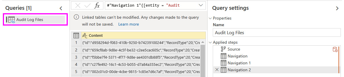
Figure 8.19 – A linked entity indicated visually

• Enhanced Compute and Computed Entities: Premium dataflows can take advantage of the Enhanced Compute Engine, which is turned on by default for Premium. This can dramatically reduce refresh time for long-running transformations such as performing joins, using distinct filters and grouping. Power BI does this by using a SQL-like cache that can handle query folding. The following screenshot shows the dataflow settings page and where to enable enhanced compute:

Figure 8.20 – Enhanced compute in the dataflow settings

Note

The enhanced compute engine setting only works when using other dataflows as a source. You can tell that you have a computed entity when you see the lightning symbol on top of its icon, as shown in the following screenshot. It also shows how Power BI provides a tooltip when hovering over the Source step, which indicates it will be evaluated externally.

The following screenshot highlights how computed entities are displayed in the UI:

Figure 8.21 – A computed entity indicated visually

• DirectQuery for dataflows: When using computed entities as a source for Power BI datasets, it is possible to use them in DirectQuery mode. This is useful when you have many refreshing datasets that rely on a dataflow. Even though the dataflow is only loaded from the external data source into Power BI once, switching to DirectQuery could reduce the load on both Power BI and the source. In Kimball dimensional modeling terms, this is useful when you have large dimensions but often query a relatively small number of them and don't need most of their attributes. We will discuss dimensional modeling in further detail, in Chapter 10, Data Modeling and Row-Level Security.

DirectQuery mode is configured when accessing a dataflow as a data source in Power BI Desktop. You do this with the Power BI Dataflows connector, and you will be provided with the option to select Import mode or DirectQuery mode, the same as with other data sources that support both storage modes. Currently, there are some limitations to DirectQuery dataflows, such as the inability to use them with Import/DirectQuery composite models. Please refer to Microsoft's online documentation to check whether your scenario is supported.

We now have a great understanding of how data gets transformed in Power BI and how we can minimize refresh operations and make them faster. Let's wrap up the chapter with a summary of our learnings.

Summary

In this chapter, we began to dive deeper into specific areas of an actual Power BI solution, starting from transforming and loading data. We saw how Power Query and the mashup engine take center stage in this part of the pipeline, powered by the M query language. We learned how memory and CPU are important for data refresh operations. This meant that poor Power Query design can lead to failed or long-running data refreshes due to resource exhaustion.

Additionally, we learned about parallelism and how you can change the settings in Power BI Desktop to improve performance. There are also settings that can be adjusted in Power BI Desktop to speed up the developer experience and optimize data loading in general. We also learned how to customize refresh parallelism in Power BI Premium, Embedded, and Azure Analysis Services.

Then, we moved on to transformations, focusing on typical operations that can slow down with large volumes of data such as filtering, joining, and aggregating. We introduced the mashup engine's ability to perform query folding and why we should leverage this as much as possible because it pushes typically resource-intensive operations down to the data source. Such operations can often be performed far more efficiently at the data source. We learned how to see where folding is occurring in Power BI Desktop and examined how to configure incremental refresh to reduce the amount of data loaded.

The Power Query diagnostic logs contain information about each query step and its resource usage. We saw how these were not easy to parse and structure, but they do offer a lot of detail that can provide valuable insights into slow query steps or data sources.

We concluded the chapter by learning how dataflows can be used to reduce data loading and transformation by centralizing common logic and data. Also, we learned how dataflows benefit from the same performance guidance as Power Query tables. However, dataflows do have their own optimization tips with specific performance features such as enhanced compute.

Now that we have learned how to get data into Power BI efficiently, in the next chapter, we will look at report and dashboard design tips to provide a better user experience while reducing data consumption.