
Model analytics for defect prediction based on design-level metrics and sampling techniques
Aydin Kayaa; Ali Seydi Kecelia; Cagatay Catalb; Bedir Tekinerdoganb aDepartment of Computer Engineering, Hacettepe University, Ankara, Turkey
bInformation Technology Group, Wageningen University, Wageningen, The Netherlands
Abstract
Predicting software defects in the early stages of the software development life cycle, such as the design and requirement analysis phase, provides significant economic advantages for software companies. Model analytics for defect prediction lets quality assurance groups build prediction models earlier and predict the defect-prone components before the testing phase for in-depth testing. In this study, we demonstrate that Machine Learning-based defect prediction models using design-level metrics in conjunction with data sampling techniques are effective in finding software defects. We show that design-level attributes have a strong correlation with the probability of defects and the SMOTE data sampling approach improves the performance of prediction models. When design-level metrics are applied, the Adaboost ensemble method provides the best performance to detect the minority class samples.
Keywords
defect prediction; design-level metrics; sampling techniques; software defects; model analytics
6.1 Introduction
Software defect prediction is a quality assurance activity which applies historical defect data in conjunction with software metrics [1–3]. It identifies which software modules are defect-prone before the testing phase, and then quality assurance groups allocate more testing resources into these modules because the other group of modules, called nondefect-prone, will not likely cause defects based on the output of the prediction approach [4]. Most of the studies in literature use classification algorithms in Machine Learning to classify software modules into two categories (defect-prone and nondefect-prone) [1].
Prior defects and software metrics data are mostly stored in different repositories, namely, bug tracking systems and source code repositories, and the processing of these data depends on the underlying platforms. Sometimes the mapping of each defect into the appropriate source code introduces errors and it is not a trivial task. While this defect prediction activity provides several benefits to organizations, only a limited number of companies have yet adopted this approach as part of their daily development practices. One strategy to increase the adoption of these approaches is to develop new models to increase the performance of existing defect prediction models.
In this study, we focus on data sampling techniques for the improvement because defect prediction datasets are always unbalanced, which means that approximately 10–20% of modules belong to the defect-prone category. While there are several attempts to apply sampling techniques in this domain, there is not an in-depth study which analyzes several classification algorithms in conjunction with design-level metrics and sampling approaches. Hence, we performed several experiments on ten public datasets by using six classification algorithms and design-level metrics.
The object-oriented Chidamber–Kemerer (CK) metrics suite, which includes six class-level metrics, is used in this study. Since datasets include additional features such as lines of code, we performed another case study to compare prediction models having the total set of features. We adopted the following classification algorithms because they have been widely used in defect prediction studies: AdaBoostM1, Linear Discriminant, Linear Support Vector Machine (SVM), Random Forest, Subspace Discriminant, and Weighted-kNN (W-kNN). The following six performance evaluation parameters are used to evaluate the performance of models: Area under ROC Curve (AUC), Recall, Precision, F-score, Sensitivity, and Specificity [5].
We analyzed the effects of the following sampling methods on the performance of defect prediction models using design-level metrics: ADASYN, Borderline SMOTE, and SMOTE. We compared their performance against the ones built based on the unbalanced data.
Our research questions are given as follows:
- • RQ1: Which sampling techniques are more effective to improve the performance of defect prediction models?
- • RQ2: Which classifiers are more effective in predicting software defects when sampling techniques are applied?
- • RQ3: Are design-level metrics (CK metrics suite) suitable to build defect prediction models when sampling techniques are applied?
The contribution of this chapter is two-fold:
- • The effects of sampling techniques are investigated for software defect prediction problem in detail.
- • The effects of six classification algorithms and design-level software metrics are evaluated on ten public datasets.
This paper is organized as follows: Section 6.2 explains the background and related work, Section 6.3 shows the methodology regarding our experimental results, Section 6.4 explains the experimental results, Section 6.5 provides the discussion, and Section 6.6 shows the conclusion and future work.
6.2 Background and related work
Software defect prediction, a quality assurance activity, identifies defect-prone modules before the testing phase and therefore, more testing resources are allocated to these modules to detect defects before the software deployment. It is a very active research field which has attracted many researchers in the software engineering community since the middle of the 2000s [4,1].
Machine Learning algorithms are widely used in these approaches and the prediction models are built using software metrics and defect labels. Software metrics can be collected at several levels, i.e., the requirements level, design level, implementation level, and process level. In the first case study of this paper, we applied the CK metrics suite, which is a set of design-level metrics. CK metrics are explained as follows:
- • The Weighted Methods per Class (WMC) metric shows the number of methods in a class.
- • The Depth of Inheritance Tree (DIT) metric indicates the distance of the longest path from a class to the root element in the inheritance hierarchy.
- • The Response For a Class (RFC) metric provides the number of available methods to respond a message.
- • The Number Of Children (NOC) indicates the number of direct descendants of a class.
- • The Coupling Between Object classes (CBO) metric indicates the number of noninheritance-related classes to which a class is coupled.
- • The Lack of COhesion in Methods (LCOM) metric indicates the access ratio of the class' attributes.
Software metrics are features of the model and the defect labels are class labels. From a Machine Learning perspective, these prediction models can be considered as classification models since we have two groups of data instances, namely, defect-prone and nondefect-prone. Defect prediction datasets are imbalanced [6], which means that most of the modules (i.e., 85–90%) in these datasets belong to the nondefect-prone class. Therefore, classification algorithms in Machine Learning might not detect the minority of data points due to the imbalanced characteristics of datasets.
The Machine Learning community has done a lot of research on the imbalanced learning so far [7,8], but the empirical software engineering community has not evaluated the impact of these algorithms in detail yet compared to the Machine Learning researchers. Algorithms in imbalanced learning can be shown in the following four categories [9]:
- 1. Subsampling [10]: With subsampling, data distribution is balanced before the classification algorithm is applied. The following four main approaches exist in this category [9]:
- (a) Under-sampling: A subset of the majority class is selected to balance the distribution of the data points, but this might cause loss of some useful data.
- (b) Over-sampling: A random replication of the minority class is created, but this might cause an over-fitting problem [11].
- (c) SMOTE [10]: This is a very popular over-sampling method and it successfully avoids over-fitting by generating new minority data points with the help of interpolation between near neighbors.
- (d) Hybrid methods [12]: These methods combine several subsampling methods to balance the dataset.
- 2. Cost-sensitive learning [13]: A false negative prediction is more costly than a false positive prediction in software defect prediction. This approach uses a cost matrix which specifies the costs of misclassification for each class, and then this matrix is applied for the optimization of the training data [9]. Since misclassification costs are not publicly available, their applications require the knowledge of domain experts.
- 3. Ensemble learning [14]: The generalization capability of different classifiers are combined, and then the new classifier, which is called ensemble of classifiers or multiple classifiers system (MCS), provides a better performance than the individual classifiers used to design it. Bagging [15] and Boosting [16] are some of the most popular algorithms used in this category. AdaBoost is shown in one of the top ten algorithms in data mining [17,9].
- 4. Imbalanced ensemble learning [11]: These algorithms combine the subsampling methods with the ensemble learning algorithms. If the over-sampling method is used in the Bagging approach instead of random sampling in Bagging, this is known as OverBagging [18]. There are several approaches which use the same idea [19–21].
In this study, we used algorithms from subsampling (ADASYN, Borderline SMOTE, and SMOTE algorithms) and ensemble learning (AdaBoostM1 algorithm) categories. We did not experiment with algorithms in the cost-sensitive learning category because there is not an easy way to identify the costs for the analysis. In addition to these algorithms, we used additional classification algorithms in conjunction with imbalanced learning algorithms. Since AdaboostM1 is an ensemble learning algorithm and we used it in conjunction with subsampling techniques, we can say that we also utilized from the category called imbalanced ensemble learning.
We applied two additional subsampling approaches, called ADASYN and Borderline SMOTE, in our study compared to the study of Song et al. [9]. Also, we applied two additional classification algorithms, called Linear Discriminant and Subspace Discriminant, which were not analyzed in the study of Song et al. [9].
6.3 Methodology
6.3.1 Classification methods
Six classification methods have been investigated in this study. These are Random Forest, Adaboost, SVM, Linear Discriminant Analysis (LDA), Subspace Discriminant, and W-kNN. Random Forest, Adaboost, and Subspace Discriminant are ensemble classification methods which combine single classifiers to obtain better predictive performance. Single classifiers during our experiments are SVM, LDA, and W-kNN. These classifiers are widely used base methods for ensemble classification. A brief description of these ensemble and single Machine Learning algorithms are provided in the following subsections.
6.3.2 Ensemble classifiers
The first ensemble method used in our experiments is Random Forest. Random Forest is a combination of multiple decision trees [22]. Bootstrapping is applied for sample selection for each tree in the forest. Two-thirds of the selected data is used to train a tree, and the classification is performed with the remaining data. Majority voting is applied to obtain the final prediction result. The Random Forest algorithm counts the votes from all the trees and the majority of the votes is used for the classification output. Random Forest is easy to use, it prevents over-fitting, and it stores the generated decision tree cluster for the other datasets.
The second ensemble method is Subspace Discriminant, which uses linear discriminant classifiers. Subspace Discriminant utilizes a feature-based bagging. In this method, feature bagging is applied to reduce the correlation between estimators; however, the difference compared to the bagging is that the features are randomly subsampled, having a replacement for each learner. Learners that are specialized on different feature sets are obtained.
The final ensemble method is Adaboost. The AdaBoost method, proposed by Freund and Schapire [23], utilizes boosting to obtain strong classifiers by combining the weak classifiers. In boosting, training data are split into parts. A predictive model is trained with the parts of the model and this model is tested with one of the remaining parts. Then, a second model is trained with the false predicted samples of the first model. This process is repeated. New models are trained with the samples falsely predicted by previous models.
6.3.3 Single classifiers
The first and most well-known single classifier used in our experiments is SVM. SVM is a common method among Machine Learning tasks [24]. In this method, the classification is performed by using linear and nonlinear kernels. The SVM method aims to find the hyperplane that separates the data points in the training set with the farthest distance.
The second single classifier is LDA. LDA projects a dataset into a lower-dimensional feature space to increase the separability between classes [25]. The first step of LDA is the computation of the variances between class features to measure the separability. The second step is to calculate the distance between the mean and samples of each class. The final step is to construct the lower-dimensional space that maximizes the interclass variance and minimizes the intraclass variance.
Our last single classifier method is W-kNN. W-kNN is an extension of the k-Nearest Neighbor algorithm. In the standard kNN, influences of all neighbors are the same although they have different individual similarity. In W-kNN, training samples which are close to the new observation have more weights than the distant ones [26].
6.4 Experimental results
During the experiments, we applied three data sampling methods and six classification methods on ten publicly available datasets. Three-fold cross-validation was applied for the evaluation of approaches. Each experiment was repeated fifty times. The experimental results are compared based on five evaluation metrics (AUC, Recall, Precision, F-score, and Specificity). The features are grouped as CK features, and ALL features include all features presented in datasets. The selected datasets are ant, arc, ivy, log4j, poi, prop, redactor, synapse, xalan, and xerces.
6.4.1 Experiments based on CK metrics
During these experiments, CK features were used and results were evaluated according to this feature set. The average scores of the classification methods on all datasets are presented in Fig. 6.1 and Table 6.1. Random Forest and Adaboost are the most successful classifiers based on the AUC metric (0.7396, 0.7269). The Adaboost classifier provides the best performance to identify the positive samples (i.e., minority class) (recall: 0.6083), however its performance is the worst for the identification of negative samples (i.e., majority class) (specificity: 0.6903). Linear Discriminant, Subspace Discriminant, and Linear SVM exhibited similar performance and their performance is better to identify the negative samples.
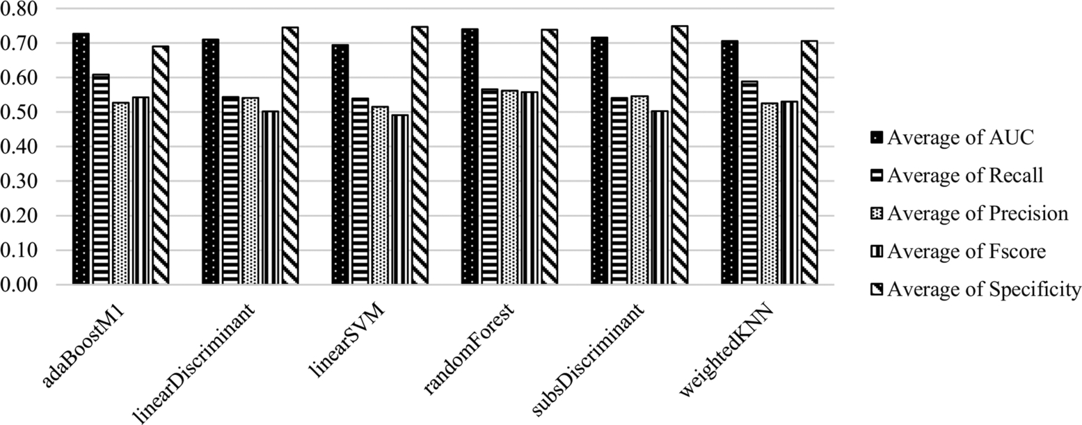
Table 6.1
Average scores of the classifiers trained and tested with CK features.
| Classifiers | Average of AUC | Average of recall | Average of precision | Average of F-score | Average of specificity |
|---|---|---|---|---|---|
| AdaBoostM1 | 0.7269 | 0.6083 | 0.5265 | 0.5429 | 0.6903 |
| Linear Discriminant | 0.7098 | 0.5435 | 0.5408 | 0.5019 | 0.7446 |
| Linear SVM | 0.6943 | 0.5397 | 0.5148 | 0.4908 | 0.7465 |
| Random Forest | 0.7396 | 0.5658 | 0.5614 | 0.5576 | 0.7381 |
| Subs Discriminant | 0.7157 | 0.5414 | 0.5458 | 0.5026 | 0.7495 |
| Weighted-kNN | 0.7057 | 0.5888 | 0.5252 | 0.5301 | 0.7062 |
The average scores of the classification methods grouped under sampling methods on all datasets are presented in Fig. 6.2 and Table 6.2. AUC and Specificity performances of the classifiers on balanced and unbalanced data are similar with improvement/decline of 1–2%. Besides, sampling methods improve the Recall metric by 13%. The effect of sampling methods is obvious on the identification of the positive samples, which is the minority class. Based on the AUC metric, SMOTE is the most successful sampling method on the datasets including CK features.
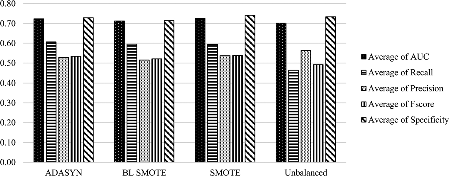
Table 6.2
Average scores of the sampling methods with CK features.
| Sampling method | Average of AUC | Average of recall | Average of precision | Average of F-score | Average of specificity |
|---|---|---|---|---|---|
| ADASYN | 0.7232 | 0.6065 | 0.5282 | 0.5342 | 0.7286 |
| BL SMOTE | 0.7121 | 0.595 | 0.5146 | 0.5208 | 0.7138 |
| SMOTE | 0.7247 | 0.5933 | 0.5374 | 0.5375 | 0.7412 |
| Unbalanced | 0.7013 | 0.4634 | 0.5628 | 0.4914 | 0.7332 |
6.4.2 Experiments based on ALL metrics
In these experiments, all of the features were used, and the results are presented according to this feature set [27]. Features and datasets can be accessed from the SEACRAFT repository http://tiny.cc/seacraft. Jureczko and Madeyski [27] used the CKJM tool to collect the 19 metrics, i.e., CK metrics suite, QMOOD metrics suite, Tang, Kao and Chen's metrics, and cyclomatic complexity, LCOM3, Ca, Ce, and LOC metrics. They collected defects using the BugInfo tool.
The average scores of the classification methods on all datasets are presented in Fig. 6.3 and Table 6.3. Random Forest and Adaboost are the most successful classifiers based on the AUC metric (0.7558, 0.7363), as in the experiments with CK features. Adaboost and Subspace Discriminant classifiers provide the best performance to identify the positive samples (recall: 0.5430, 0.5420). In contrast to the CK experiments, the Adaboost classifier is one of the best performing classifiers to identify the negative samples (specificity: 0.7576). Random Forest is the best classifier for the identification of the majority class (specificity: 0.7692). The performance of Linear SVM (AUC: 0.7116) and W-kNN (AUC: 0.6776) is lower than that of the other algorithms.
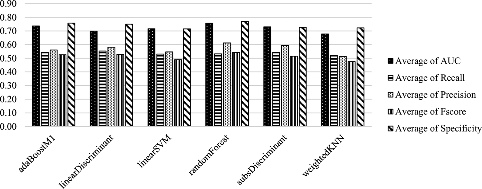
Table 6.3
Average scores of the classifiers trained and tested with ALL features.
| Classifier | Average of AUC | Average of recall | Average of precision | Average of F-score | Average of specificity |
|---|---|---|---|---|---|
| AdaBoostM1 | 0.7363 | 0.5430 | 0.5608 | 0.5256 | 0.7576 |
| Linear Discriminant | 0.6994 | 0.5530 | 0.5809 | 0.5276 | 0.7497 |
| Linear SVM | 0.7161 | 0.5309 | 0.5469 | 0.4892 | 0.7150 |
| Random Forest | 0.7558 | 0.5325 | 0.6116 | 0.5431 | 0.7692 |
| Subs Discriminant | 0.7298 | 0.5420 | 0.5946 | 0.5154 | 0.7262 |
| Weighted-kNN | 0.6776 | 0.5208 | 0.5138 | 0.4757 | 0.7223 |
The average scores of the classification methods grouped under sampling methods on all datasets are presented in Fig. 6.4 and Table 6.4. The performance of classifiers with respect to AUC and Specificity parameters on balanced (ADASYN and BL SMOTE methods) and unbalanced data are similar, with improvement/decline of 1–3%. Besides, ADASYN and BL SMOTE sampling methods improve the recall metric by 14%; however, this effect is reversed when the SMOTE method is considered. The average AUC value drops from 0.7445 to 0.6357 in the case of the SMOTE data sampling method. Precision score is the highest for the classifiers on unbalanced data. The effect of sampling methods is obvious on the identification of the positive samples which belong to the minority class. In contrast to CK experiments, SMOTE is the worst performing sampling method on the datasets including ALL features, and the recall value drops from 0.5025 to 0.3613 when SMOTE is applied. Therefore, SMOTE does not help to identify the instances belonging to the minority class when all the features are used.
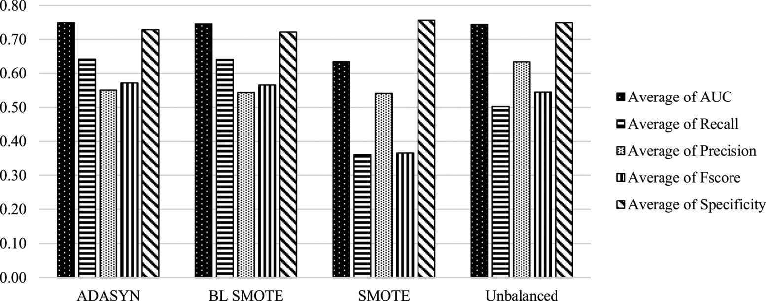
Table 6.4
Average scores of the sampling methods with ALL features.
| Sampling method | Average of AUC | Average of recall | Average of precision | Average of F-score | Average of specificity |
|---|---|---|---|---|---|
| ADASYN | 0.7499 | 0.643 | 0.5514 | 0.5728 | 0.7296 |
| BL SMOTE | 0.7465 | 0.6414 | 0.5443 | 0.5667 | 0.7233 |
| SMOTE | 0.6357 | 0.3613 | 0.5418 | 0.3663 | 0.7572 |
| Unbalanced | 0.7445 | 0.5025 | 0.6349 | 0.5452 | 0.7499 |
6.4.3 Comparison of the features
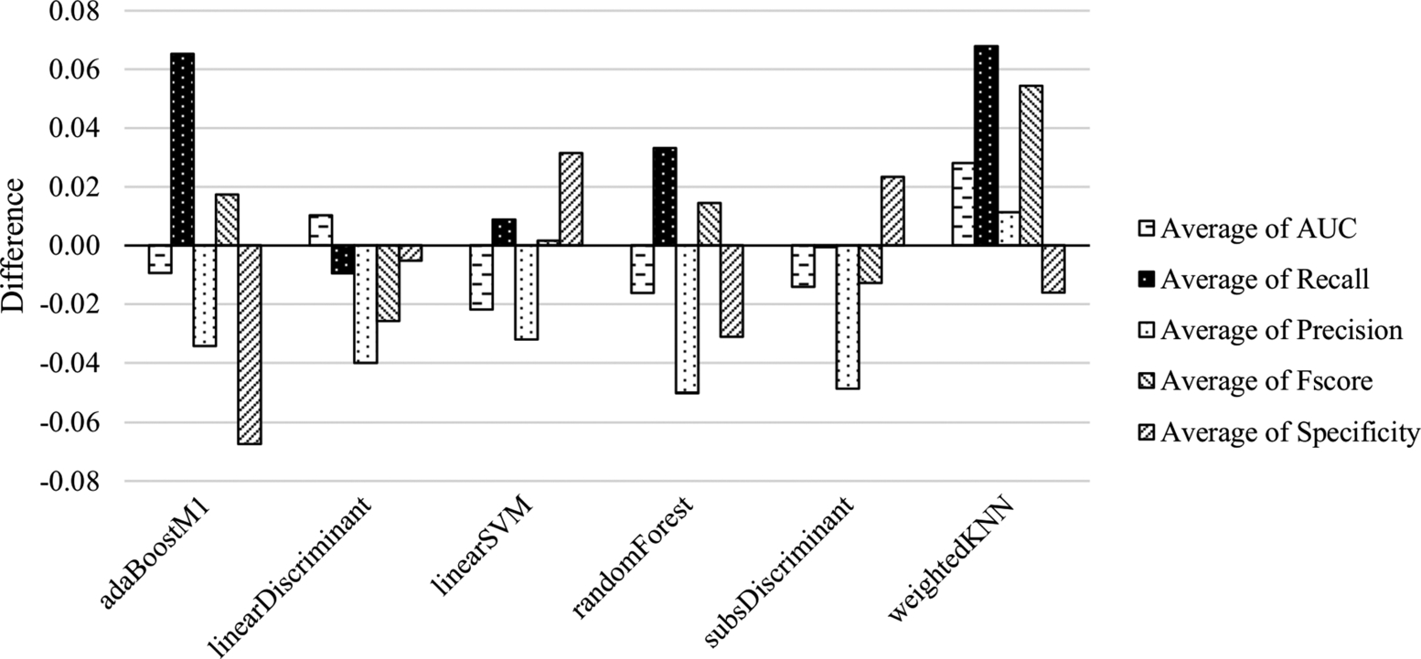
In this section, the experiments with CK and ALL features are compared. By using the values from Table 6.1 and Table 6.3, the comparison of average outcomes of the classification methods is presented in Fig. 6.5. In this figure, negative values denote the superiority of ALL features, while positive values denote the superiority of CK features. While the CK features set is more successful on the identification of the positive samples, the ALL features set is better on the negative samples. It seems that the difference with respect to AUC and F-score values is low. Besides, classifiers trained with ALL features provide better precision scores.
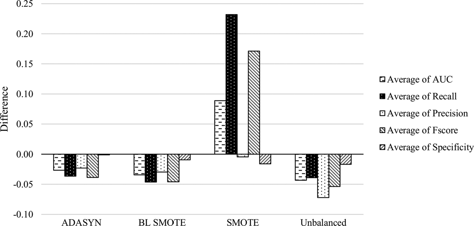
By using the values from Table 6.2 and Table 6.4, the comparison of average outcomes of the sampling methods is presented in Fig. 6.6. In this figure, negative values denote the superiority of ALL features, while positive values denote the superiority of CK features. While the classifiers trained with balanced data using the SMOTE method provided better AUC, F-score, and recall outcomes on CK features, the other sampling methods are more beneficial on ALL features and provided better outcomes for all scores.
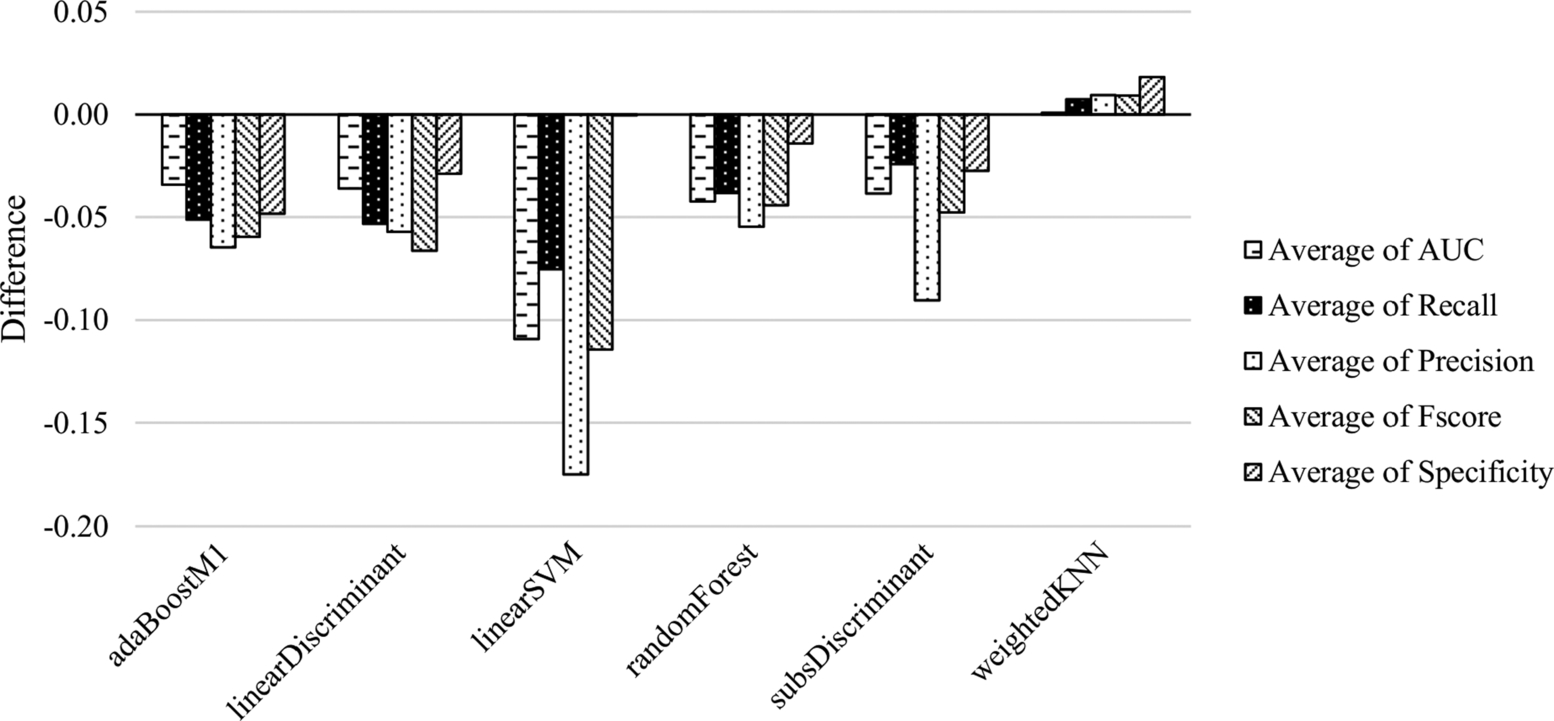
In Fig. 6.7, the difference between outcomes of the classifiers with CK and ALL features is presented on the unbalanced datasets. In this figure, negative values denote the superiority of ALL features, positive values denote the superiority of CK features. The outcomes of the classifiers with ALL features are better except the W-kNN classifier. ALL features are more preferable than CK features when it comes to dealing with unbalanced datasets.
In Table 6.5, statistical significance results obtained by McNemar's test are presented. All the classifier/sampling method combinations are compared as CK vs. ALL features for all datasets. In the table, classification methods are grouped for each data sampling method. P-values are shown for each dataset. The significant values (![]() ) are indicated as italic and boldfaced.
) are indicated as italic and boldfaced.
Table 6.5
Statistical significance analysis results according to the comparison of CK and ALL features. Classification methods are grouped under each data sampling method. P-values are denoted respectively for each dataset. Significant values are presented in italics.
| Methods | ant | arc | ivy | log4j | poi | prop | red. | syn. | xalan | xerces |
|---|---|---|---|---|---|---|---|---|---|---|
| ADASYN | ||||||||||
| AdaBoostM1 | 0.00 | 0.01 | 0.00 | 0.00 | 0.30 | 0.00 | 0.00 | 0.00 | 0.00 | 0.02 |
| Linear Discriminant | 0.00 | 0.10 | 0.79 | 0.00 | 0.00 | 0.52 | 0.00 | 0.12 | 0.00 | 0.00 |
| Linear SVM | 0.55 | 0.01 | 0.05 | 0.00 | 0.02 | 0.04 | 0.00 | 0.01 | 0.00 | 0.04 |
| Random Forest | 0.17 | 0.12 | 0.00 | 0.01 | 0.52 | 0.01 | 0.19 | 0.66 | 0.32 | 0.87 |
| Subs Discriminant | 0.00 | 0.07 | 0.47 | 0.00 | 0.00 | 0.14 | 0.00 | 0.63 | 0.00 | 0.20 |
| Weighted-kNN | 0.08 | 1.00 | 0.52 | 0.37 | 0.68 | 0.92 | 0.26 | 0.00 | 0.00 | 0.39 |
| BL SMOTE | ||||||||||
| AdaBoostM1 | 0.00 | 0.01 | 0.00 | 0.00 | 0.23 | 0.00 | 0.00 | 0.23 | 0.01 | 0.64 |
| Linear Discriminant | 0.00 | 0.03 | 1.00 | 0.00 | 0.00 | 0.88 | 0.00 | 0.90 | 0.00 | 0.00 |
| Linear SVM | 0.02 | 0.02 | 0.49 | 0.02 | 0.00 | 0.46 | 0.00 | 0.20 | 0.00 | 0.71 |
| Random Forest | 1.00 | 0.03 | 0.26 | 0.17 | 0.72 | 0.73 | 0.00 | 0.05 | 0.03 | 0.40 |
| Subs Discriminant | 0.00 | 0.58 | 0.65 | 0.00 | 0.00 | 0.49 | 0.00 | 0.15 | 0.00 | 0.87 |
| Weighted-kNN | 0.70 | 0.30 | 0.28 | 0.44 | 0.68 | 0.06 | 0.88 | 0.82 | 0.00 | 0.48 |
| SMOTE | ||||||||||
| AdaBoostM1 | 0.00 | 0.00 | 0.00 | 0.00 | 0.00 | 0.00 | 0.00 | 0.00 | 0.00 | 0.00 |
| Linear Discriminant | 0.00 | 0.00 | 0.00 | 0.00 | 0.00 | 0.00 | 0.00 | 0.00 | 0.23 | 0.00 |
| Linear SVM | 0.00 | 0.00 | 0.00 | 0.00 | 0.00 | 0.00 | 0.00 | 0.00 | 0.00 | 0.00 |
| Random Forest | 0.00 | 0.00 | 0.00 | 0.00 | 0.00 | 0.00 | 0.00 | 0.00 | 0.00 | 0.00 |
| Subs Discriminant | 0.00 | 0.00 | 0.00 | 0.00 | 0.00 | 0.00 | 0.00 | 0.00 | 0.00 | 0.00 |
| Weighted-kNN | 0.00 | 0.00 | 0.00 | 0.00 | 0.00 | 0.00 | 0.00 | 0.00 | 0.00 | 0.00 |
| Unbalanced | ||||||||||
| AdaBoostM1 | 0.01 | 0.18 | 0.43 | 0.37 | 0.39 | 0.62 | 0.06 | 0.37 | 0.41 | 0.32 |
| Linear Discriminant | 0.85 | 1.00 | 0.82 | 0.18 | 0.00 | 0.03 | 0.00 | 0.03 | 0.16 | 0.00 |
| Linear SVM | 0.17 | 0.16 | 0.00 | 0.45 | 0.00 | 0.55 | 0.00 | 0.49 | 0.60 | 0.35 |
| Random Forest | 1.00 | 0.05 | 0.32 | 0.26 | 0.90 | 0.00 | 0.80 | 0.63 | 0.45 | 0.47 |
| Subs Discriminant | 0.03 | 0.21 | 0.10 | 0.32 | 0.00 | 0.53 | 0.01 | 1.00 | 0.44 | 0.00 |
| Weighted-kNN | 0.92 | 0.78 | 0.68 | 0.10 | 0.01 | 0.42 | 0.78 | 0.58 | 0.56 | 0.06 |
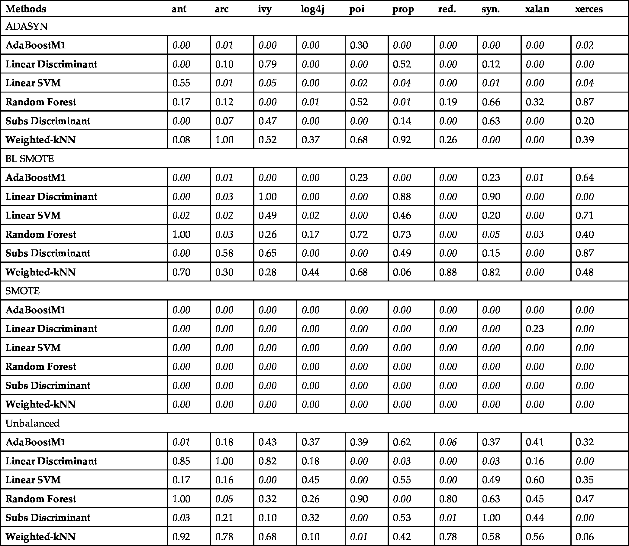
Based on Table 6.5, Fig. 6.5, and Fig. 6.6, we conclude that the SMOTE sampling method provides 100% significant values for our experiments, and this significance shows the superiority of the data with CK features when it is balanced using the SMOTE method. For other sampling methods and unbalanced data, the significant instances are also present, but there are some insignificant ones too. ALL features provide better outcomes on the unbalanced data and the balanced data with data sampling methods except SMOTE.
6.5 Discussion
In this study, we performed several experiments to evaluate the effect of design-level metrics and data sampling methods on the performance of defect prediction models. Research questions of this study were introduced in Section 6.1, and in this section we present our responses to each of them.
- • RQ1: Which sampling techniques are more effective to improve the performance of defect prediction models?
- The answer to RQ1: Regarding the CK metrics suite, the SMOTE data sampling method is the best one; for the ALL metrics suite, the other data sampling methods are preferable.
- • RQ2: Which classifiers are more effective in predicting software defects when sampling techniques are applied?
- The answer to RQ2: Regarding the CK metrics, the Random Forest algorithm is the most effective one with respect to the AUC value. Adaboost is the second best performing algorithm and it is also the best algorithm to identify the minority class instances.
- Regarding the ALL metrics set, again the Random Forest algorithm provides the best performance and Adaboost is the second best performing one. Adaboost and Linear Discriminant are the best performing algorithms for the identification of minority class instances. For the detection of majority class instances, Adaboost is the best classifier.
- • RQ3: Are design-level metrics (CK metrics suite) suitable to build defect prediction models when sampling techniques are applied?
- The answer to RQ3: We showed that the CK features set is more successful for the identification of minority class instances and the ALL features set is better for the identification of majority class instances. When CK metrics are used with the Random Forest algorithm, the best performance was achieved using the CK metrics suite. When additional features are added to the CK metrics suite, the performance of a Random Forest-based model with respect to AUC value improved from 0.7396 to 0.7558.
Potential threats to validity for this study are evaluated from four dimensions, namely, conclusion validity, construct validity, internal validity, and external validity [28]. Regarding the conclusion validity, we applied a three-fold cross-validation evaluation technique 50 times (N * M cross-validation, N = 3, M = 50) to get statistically significant results and avoid randomness during the experiments. In addition to this validation technique, we performed McNemar's test to evaluate the statistical significance of our results. Five evaluation parameters were used to report the experimental results and ten public datasets were investigated. For the construct validity dimension, we can state that we applied the widely used ten public datasets for the software defect prediction problem. Regarding the internal validity, we investigated three single classifiers, three ensemble techniques, and three data sampling techniques in this study to evaluate the impact of classifiers, metrics suite, and data sampling techniques on software defect prediction. While we selected the best performing algorithms, other researchers might analyze the other techniques with different parameters and therefore, they can obtain different results. For the external validity dimension, we must stress that our conclusions are valid on datasets explained in the paper and results might be different on a different set of datasets.
6.6 Conclusion
Software defect prediction is an active research problem [29,9,30–33]. Hundreds of papers on this problem have been published so far [32]. In this study, we focused on the impact of data balancing methods, ensemble methods, and single classification algorithms for software defect prediction problems. We empirically showed that design-level metrics can be used to build defect prediction models. In addition, when design-level metrics (CK metrics suite) are applied, we demonstrated that the SMOTE data sampling approach can improve the performance of prediction models. Among other ensemble methods, we observed that the Adaboost ensemble method is the best one to identify the minority class (defect-prone) samples when the CK metrics suite is adopted. When all metrics in the dataset are applied, the Adaboost algorithm provides the best performance to identify the majority class instances. In the near future, we will perform more experiments when we access more data balancing methods and more datasets on this issue.