Chapter 3. Modeling and Analysis with the AADL: The Basics
In this chapter, we illustrate the development of basic AADL models and present general guidance on the use of some of the AADL’s core capabilities. With this, we hope to provide a basic understanding of architectural modeling and analysis and start you on your way in applying the AADL to more complex software-dependent systems.
While reading the first part of this chapter, you may want to use an AADL development tool to create the specifications and conduct the analyses described. OSATE supports all of the modeling and analyses discussed in this chapter.
3.1. Developing a Simple Model
In this section, we present a step-by-step development and analysis of an AADL model. Specifically, we model a control system that provides a single dimension of speed control and demonstrate some of the analyses that can be conducted on this architectural model. The speed control functionality is part of a powerboat autopilot (PBA) system that is detailed in Appendix A. While specialized to a powerboat, this model exemplifies the use of the AADL for similar control applications such as aeronautical, automotive, or land vehicle speed control systems.
The approach we use is introductory, demonstrating the use of some of the core elements and capabilities of the AADL. We do not include many of the broader engineering capabilities of the language. For example, we do not address packages, prototypes, or component extensions in developing this simple model. These are discussed later in this chapter. Instead, we proceed through the generation of a basic declarative model and its instance and show a scheduling analysis of the system instance. During your reading of this section, you may want to reference Part II for details on specific AADL elements or analyses used in the example.
Initially we create a high-level system representation using AADL system, process, and device components. Building on this initial representation, we detail the runtime composition of all of the elements; allocate software to hardware resources; and assign values to properties of elements to a level that is required for analysis and for the creation of an instance of the system. In these steps, we assume that requirements are sufficiently detailed to provide a sound basis for the architectural design decisions and trade-offs illustrated in the example. In addition, while we reference specific architectural development and design approaches that put the various steps into a broader context, we do not advocate one approach over another.
3.1.1. Defining Components for a Model
A first step is to define the components that comprise the system and place their specification in packages. The process of defining and capturing components is similar to identifying objects in an object-oriented methodology. It is important to realize that components may include abstract encapsulations of functionality as well as representations of tangible things in the system and its environment. The definition of components is generally an iterative and incremental process, in that the first set of components may not represent a complete set and some components may need to be modified, decomposed, or merged with others.
First, we review the description of the speed controller for the PBA and define a simplified speed control model. In this model, we include a pilot interface unit for input of relevant PBA information, a speed sensor that sends speed data to the PBA, the PBA controller, and a throttle actuator that responds to PBA commands.
For each of the components identified, we develop type definitions, specifically defining the component’s name, runtime category, and interfaces. Since we are initially developing a high-level (conceptual) model, we limit the component categories to system, process, and device.
The initial set of components is shown in Table 3-1, where both the AADL text and corresponding graphical representations are included. For this example, the textual specifications of all of the components required for the model are contained in a single package and no references to classifiers outside the package are required. Thus, a package name is not needed when referencing classifiers. For the graphical representations, the implementation relationship is shown explicitly. Note that the icon for an implementation has a bold border when compared to the border of its corresponding type icon.
Table 3-1. Component Type and Implementations for the Speed Control Example
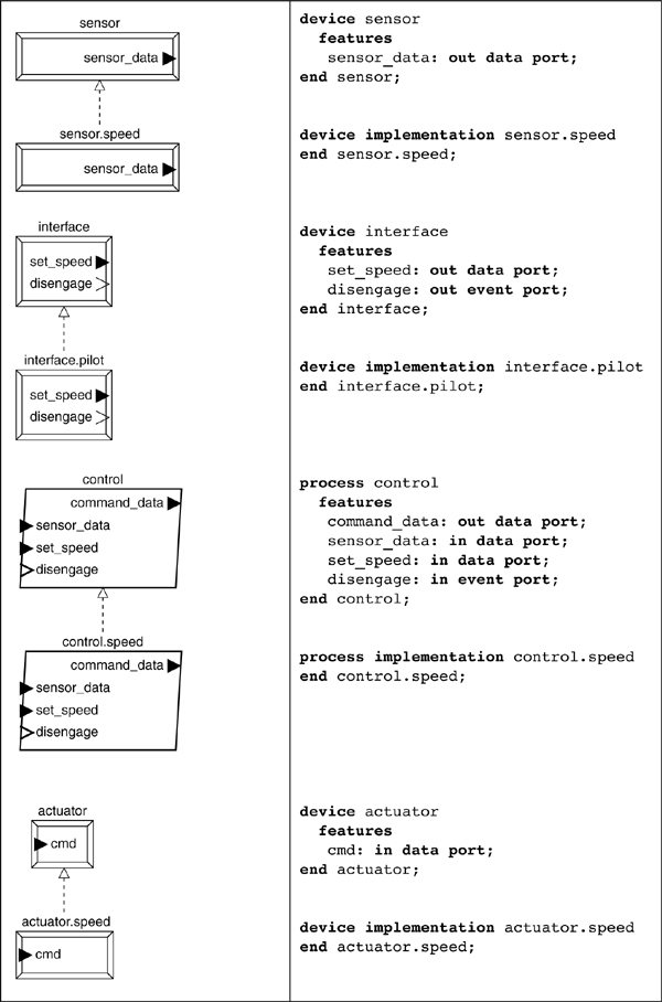
The speed sensor, pilot interface, and throttle actuator are modeled as devices and the PBA control functions are represented as a process. We use the devices category for components that are interfaces to the external environment that we do not expect to decompose extensively (e.g., a device can only have a bus as a subcomponent).
Devices in AADL can represent abstractions of complex components that may contain an embedded processor and software. With a device component, you represent only those characteristics necessary for analysis and an unambiguous representation of a component. For example, in modeling a handheld GPS receiver, we may only be interested in the fact that position data is available at a communication port. The fact that the GPS receiver has an embedded processor, memory, touch screen user interface, and associated software is not required for analysis or modeling of the system. Alternatively, a device can represent relatively simple external components, such as a speed sensor, whose only output is a series of pulses whose frequency is proportional to the speed being sensed. If you require a complex interface to the external environment, you can use a system component. In this case, you can detail its composition and as needed include an uncomplicated device subcomponent to represent the interface to the environment.
The use of a process component for the control functions reflects the decision that the core control processing of the PBA is to be implemented in software. The software runtime components will be contained within an implementation of this process type. The implementation declarations in Table 3-1 do not include any details. As the design progresses, we will add to these declarations (i.e., adding subcomponents and properties as appropriate).
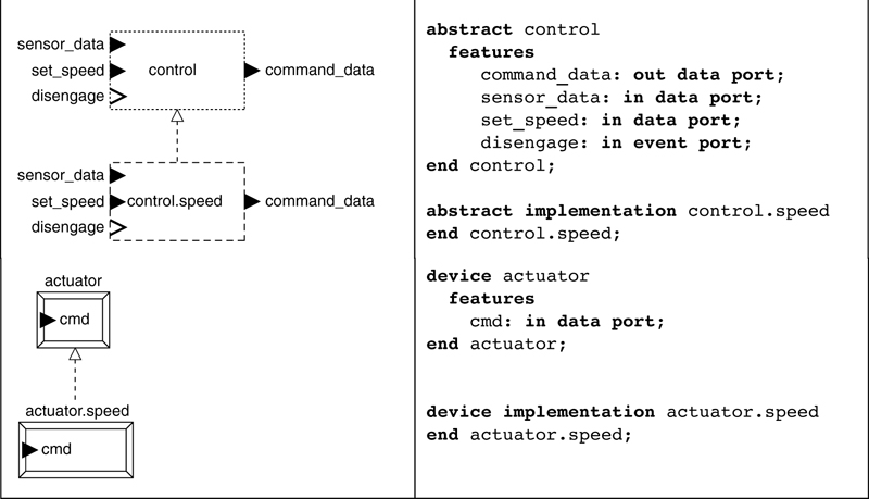
The interfaces for the PBA components are port features declared within a component type and are reflected in each implementation of that type. For example, the type sensor outputs a value of the speed via a data port sensor_data. The pilot interface type interface provides a value for the set speed via a data port set_speed and generates a signal to disengage the speed control via an event port disengage.
Notice that we have used explicit as well as abbreviated naming for the ports and other elements of the model (e.g., command_data and cmd for the command data at input and output ports). The specificity of names is up to you, provided they comply with AADL naming constraints for identifiers (e.g., the initial character cannot be a numeral). Note that naming is case insensitive and Control is the same name as control.
In the PBA example, we have chosen to assign specific runtime component categories to each of the components (e.g., the speed sensor is a device). However, in real-world development as a design matures, the definition of these components may change (e.g., a component that computes the PBA speed control laws may initially be represented as a system and later modified to a process or thread). Using the approach we outline here, these changes are done manually within the AADL model (i.e., changing a system declaration to a process category declaration). An alternative approach is to use the generic abstract component category (i.e., not defining a specific runtime essence). Then later in the development, converting this abstract category into a specific runtime category employing the AADL extends capability (e.g., converting an abstract component to a thread). We have chosen to use the former approach to simplify the presentation and focus on decisions and issues related to representations of the system as concrete runtime components. A discussion of the use of the abstract component category is provided in Section 3.5.
For each of the component types we define a single implementation. These declarations are partial, in that we omit substantial details needed for a complete specification of the architecture. For example, we do not define the type of data that is associated with the ports. We will address these omissions as required in later steps. However, we can conduct a number of analyses for our simple example without including many of these details.
3.1.2. Developing a Top-Level Model
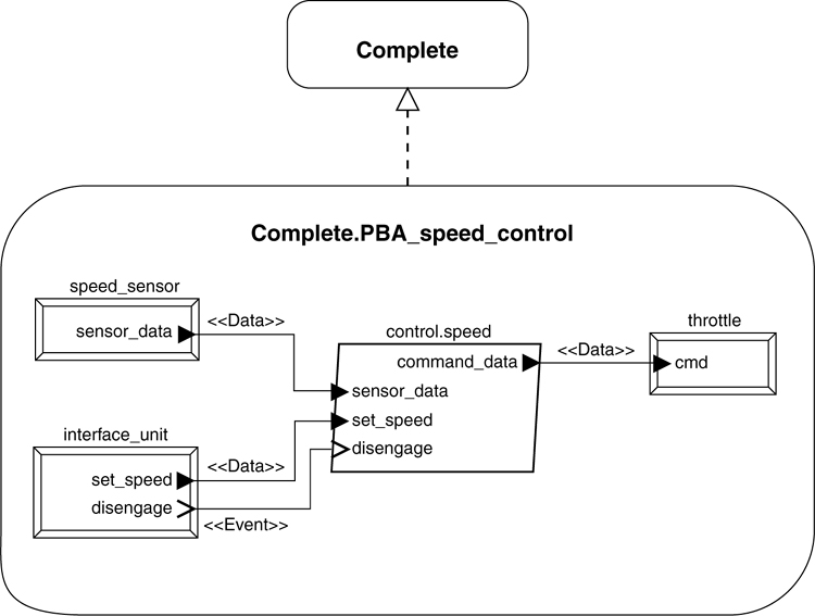
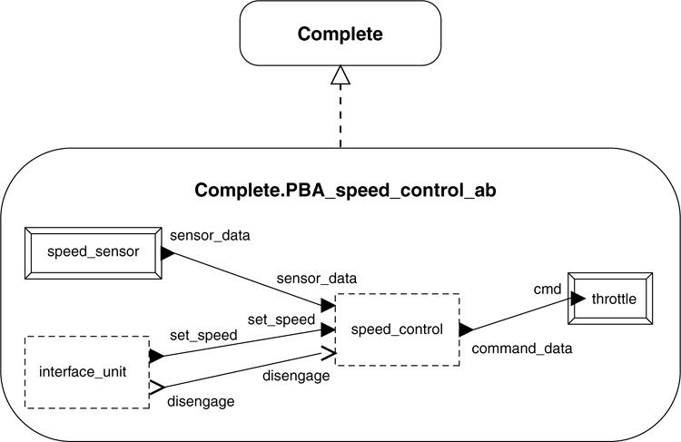
In the next step, we integrate the individual component implementations into a system by declaring subcomponents instances and their connections. We do this by defining an enclosing system type and implementation as shown in Listing 3-1, where we define a system type Complete and its implementation Complete.PBA_speed_control. There is nothing special about our choice of naming for this enclosing system. Another naming scheme, such as a type of PBA and an implementation of PBA.speed, would work as well.
Within the implementation, we declare four subcomponents. The three device subcomponents represent the speed sensor, throttle, and the pilot interface unit. The process subcomponent speed_control represents the software that provides the speed control for the PBA. Notice that there are no external interfaces for the system type Complete. All of the interactions among the system’s subcomponents are internal to the implementation Complete.PBA_speed_control, with the devices that comprise the system providing the interfaces to the external environment (e.g., sensors determining speed information from the vehicle).
Within the implementation, we define connections for each of the ports of the subcomponents. For example, connection DC2 is the data connection between the command_data port on the process speed_control and the cmd data port on the device throttle. Each of the connections is labeled in the graphical representation shown in Listing 3-1 by the nature of the connection.1 For example, connection EC4 between the event port disengage on the interface_unit device and the event port disengage on the speed_control process is labeled as <<Event>>. It is our choice to match most of the port names. It is not required that connected ports have the same name. However, they must have matching data classifiers if specified (they are omitted in this initial representation).
Listing 3-1. Subcomponents of the Complete PBA System
system Complete
end Complete;
system implementation Complete.PBA_speed_control
subcomponents
speed_sensor: device sensor.speed;
throttle: device actuator.speed;
speed_control: process control.speed;
interface_unit: device interface.pilot;
connections
DC1: port speed_sensor.sensor_data ->
speed_control.sensor_data;
DC2: port speed_control.command_data -> throttle.cmd;
DC3: port interface_unit.set_speed ->
speed_control.set_speed;
EC4: port interface_unit.disengage ->
speed_control.disengage;
end Complete.PBA_speed_control;
Depending upon your development environment the graphical portrayals may differ from those shown in Listing 3-1. For example, within OSATE you cannot display the containment explicitly. Rather, the internal structure of an implementation is presented in a separate diagram that can be accessed hierarchically through the graphical icon representing the implementation Complete.PBA_speed_control.
3.1.3. Detailing the Control Software
At this point, we begin to detail the composition of the process speed_control. This involves decisions relating to partitioning the functionality and responsibilities required of the PBA system to provide speed control. Since we have treated the speed control as an autonomous capability, we have implicitly assumed that there are no interactions between the directional or other elements of the PBA and the speed control system. This may not be the case in advanced control systems. In addition, for the purposes of this example, we partition the functions of the speed control process into two subcomponents. The first is a thread that receives input from speed sensor; scales and filters that data; and delivers the processed data to the second thread. The second is a thread that executes the PBA speed control laws and outputs commands to the throttle actuator. Again, this simplification may not be adequate for a realistic speed control system (e.g., the control laws may involve extensive computations that for efficiency must be separated into multiple threads or may involve complex mode switches that are triggered by various speed or directional conditions)2.
Since the interfaces for the two threads are different, we define a type and implementation for each, as shown in Listing 3-2. We have used property associations to assign execution characteristics to the threads. Each is a periodic thread (assigned using the Dispatch Protocol property association) with a period of 50ms (assigned using the Period property association).
Listing 3-2. PBA Control Threads Declarations
thread read_data
features
sensor_data: in data port;
proc_data: out data port;
properties
Dispatch_Protocol => Periodic;
Period => 50 ms;
end read_data;
thread implementation read_data.speed
end read_data.speed;
thread control_laws
features
proc_data: in data port;
cmd: out data port;
disengage: in event port;
set_speed: in data port;
properties
Dispatch_Protocol => Periodic;
Period => 50 ms;
end Control_laws;
thread implementation control_laws.speed
end control_laws.speed;
The assignment of periodic execution and the values for the period of the threads reflect design decisions. Generally, these are based upon the input of application domain and/or control engineers. The assignments we use here are not necessarily optimal but are chosen to provide specific values to enable analysis of system performance. They do not reflect the values for any specific control system.
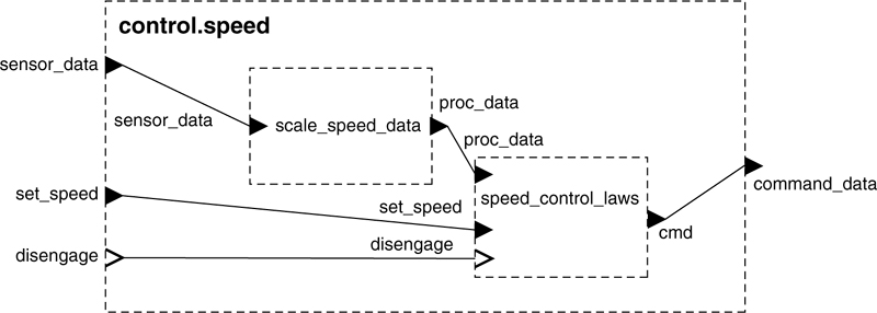
We detail the declaration of the process implementation control.speed that is presented in Table 3-1 to include the two thread subcomponents and their interactions (connections), as shown in Listing 3-3. There are five connections declared. Four of these connect ports on the boundary of the process with ports on the threads (i.e., DC1, DC3, DC4, and EC1). The fifth connects the out data port proc_data on the thread scale_speed_data to the in data port proc_data on the thread speed_control_laws.
Listing 3-3. The Process Implementation control.speed
process implementation control.speed
subcomponents
scale_speed_data: thread read_data.speed;
speed_control_laws: thread control_laws.speed;
connections
DC1: port sensor_data -> scale_speed_data.sensor_data;
DC2: port scale_speed_data.proc_data ->
speed_control_laws.proc_data;
DC3: port speed_control_laws.cmd -> command_data;
EC1: port disengage -> speed_control_laws.disengage;
DC4: port set_speed -> speed_control_laws.set_speed;
end control.speed;

3.1.4. Adding Hardware Components
At this point, we have defined the software components of the speed control system. We now define the execution hardware required to support the software. In modeling the hardware and binding the control software to that hardware, we can analyze the execution timing and scheduling aspects of the system.
In Listing 3-4, we define a processor, memory, and bus. The processor will execute the PBA control code (threads) and the memory will store the executable code (process) for the system. In addition, we have declared that the processor type Real_Time and the memory type RAM require access to an instance of the bus implementation Marine.Standard. This bus will provide the physical pathway for the system. We will add properties to these declarations later in the modeling process.
Listing 3-4. Execution Platform Declarations
processor Real_Time
features
BA1: requires bus access Marine.Standard;
end Real_Time;
processor implementation Real_Time.one_GHz
end Real_Time.one_GHz;
memory RAM
features
BA1: requires bus access Marine.Standard;
end RAM;
memory implementation RAM.Standard
end RAM.Standard;
bus Marine
end Marine;
bus implementation Marine.Standard
end Marine.Standard;
3.1.5. Declaring Physical Connections
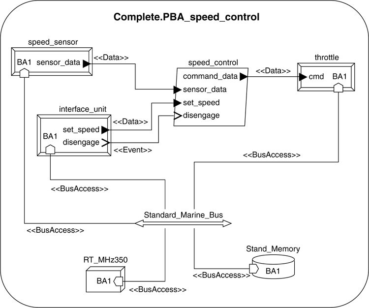
To continue the integration of the system, we add instances of the required execution platform components into the system implementation Complete.PBA_speed_control by declaring subcomponents for the implementation. In addition, we declare that these components are attached to the bus. This is done by connecting the requires interfaces on the processor and memory components to the bus component.
Since the PBA control software executing on the processor must receive data from the sensors and pilot interface unit as well as send commands to the throttle actuator, we declare that these sensing and actuator devices are connected to the bus as well. To do this, we add requires bus access declarations in the type declarations for these three devices and connect them to the bus. The updated declarations for the three devices are shown in Listing 3-5 and the graphical representation of the system with the declaration of the physical (bus access) connections is shown in Listing 3-6.
Listing 3-5. Updated Device Declarations
device interface
features
set_speed: out data port;
disengage: out event port;
BA1: requires bus access Marine.Standard;
end interface;
device sensor
features
sensor_data: out data port;
BA1: requires bus access Marine.Standard;
end sensor;
device actuator
features
cmd: in data port;
BA1: requires bus access Marine.Standard;
end actuator;
In Listing 3-6, we have defined a processor RT_1GHz3, bus Standard_Marine_Bus, and memory Stand_Memory as subcomponents. In addition, we have declared the connections for the bus Standard_Marine_Bus to the requires bus access features of each of the physical components (e.g., from Standard_Marine_Bus to RT_GHz.BA1 and to the requires bus access feature on the processor RT_1GHz.BA1). The requires access features and the bus access connections are shown in the graphical representation in the lower portion of Listing 3-6.
Listing 3-6. Integrated Software and Hardware System
system implementation Complete.PBA_speed_control
subcomponents
speed_sensor: device sensor.speed;
throttle: device actuator.speed;
speed_control: process control.speed;
interface_unit: device interface.pilot;
RT_1GHz: processor Real_Time.one_GHz;
Standard_Marine_Bus: bus Marine.Standard;
Stand_Memory: memory RAM.Standard;
connections
DC1: port speed_sensor.sensor_data ->
speed_control.sensor_data;
DC2: port speed_control.command_data -> throttle.cmd;
DC3: port interface_unit.set_speed ->
speed_control.set_speed;
EC4: port interface_unit.disengage ->
speed_control.disengage;
BAC1: bus access Standard_Marine_Bus <-> speed_sensor.BA1;
BAC2: bus access Standard_Marine_Bus <-> RT_1GHz.BA1;
BAC3: bus access Standard_Marine_Bus <-> throttle.BA1;
BAC4: bus access Standard_Marine_Bus <-> interface_unit.BA1;
BAC5: bus access Standard_Marine_Bus <-> Stand_Memory.BA1;
end Complete.PBA_speed_control;
3.1.6. Binding Software to Hardware
In addition to specifying the physical connections, we bind software components to the appropriate physical hardware using contained property associations, as shown in Listing 3-7. These property associations are added to the system implementation declaration Complete.PBA_speed_control. The first two declarations allow the threads speed_control_laws and scale_speed_data to be bound to the processor rt_mhz500. The reference part of the property association identifies the specific processor instance rt_mhz500 and the applies to identifies the specific thread in the hierarchy (e.g., applies to speed_control.scale_speed_data identifies the thread scale_speed_data that is located in the process speed_control). In this notation, a period separates the elements in the hierarchy.
We could have specified a specific binding using the Actual_Processor_Binding property. However, the Allowed_Processor_Binding property permits scheduling tools to assign the threads to processors. For example, the resourced allocation and scheduling analysis plug-in that is available in the OSATE environment4 binds threads to processors taking into consideration the threads’ period, deadline, and execution time; processor(s) speed and scheduling policies; and the constraints imposed by the actual and allowed binding properties5. Specifically, if only allowed processor bindings are defined (i.e., the Allowed_Processor_Binding property), the plug-in schedules the thread onto processors and reports back the actual thread to processor bindings and the resulting processor utilizations. If actual processor bindings are defined (i.e., the Actual_Processor_Binding property) the plug-in reports processor utilization based upon those bindings; allocates threads to processors; and runs a scheduling analysis to determine whether the bindings are acceptable.
Generally, a scheduling analysis or scheduling tool does scheduling analysis such that given a set of threads and their binding to processors (allowed or actual bindings), requisite attributes of the threads and processors (e.g., period, worst case execution time, processor cycle time, etc.), and defined scheduling policy, it determines if the set of threads meets the system’s timing requirements. Typical scheduling policies include round-robin (RR), shortest job first (SJF), earliest deadline first (EDF), and rate monotonic (RM). The specific information required by and output from scheduling analysis tools vary.
The OSATE resource allocation and scheduling analysis plug-in makes binding decisions and in that process runs a scheduling analysis determining whether the binding is acceptable. This can be based on earliest deadline first (EDF) and rate monotonic scheduling (RMS) for periodic threads. In addition, it can conduct a rate monotonic analysis for periodic threads. This is useful for control system applications where all tasks are periodic, such as the PBA speed control example. In cases where threads are already bound to processors (i.e., using the Actual_Processor_Binding property), the plug-in determines schedulability for that specific deployment configuration.
If priority is assigned by hand and rate monotonic scheduling is used, another OSATE plug-in (priority inversion checker) enables the determination of whether the system has potential priority inversion. More sophisticated schedulability analysis tools are available for analyzing AADL models. A listing of these is available at https://wiki.sei.cmu.edu/aadl.
The third entry in Listing 3-7, binds the code and data within the process speed_control to the memory component Standard_Memory. We chose to use the actual rather than the allowed memory binding property, since there is only one memory component in the system and, while an additional processor might be added, we do not anticipate additional memory components to be added.
Listing 3-7. Binding Property Associations
properties
Allowed_Processor_Binding => (reference(RT_1GHz))
applies to speed_control.speed_control_laws;
Allowed_Processor_Binding => (reference(RT_1GHz))
applies to speed_control.scale_speed_data;
Actual_Memory_Binding => (reference(Stand_Memory))
applies to speed_control;
3.1.7. Conducting Scheduling Analyses
Having defined the threads and established their allowed bindings to processors, we can begin to assess processor loading and analyze the schedulability of the system.
Before we proceed with a scheduling analysis, we define the requisite execution characteristics for the threads as they relate to the capabilities of the processors to which they may be bound. We specify this information through properties of the threads and processors. In this case, there is only one processor with an execution speed of 1GHz, as shown in Listing 3-8. Both threads are declared as Periodic with a period of 50ms. The default value in the AADL standard for the Deadline is the value of the Period. This value can be overridden by assigning a value to the Deadline using a property association. The execution time of the read_data thread ranges from 1 millisecond (ms) to 2 milliseconds (ms), whereas the control_laws thread’s execution time ranges from 3ms to 5ms (as assigned using the Compute_Execution_Time property associations). These execution times are relative to the processor Real_Time.one_GHz declared in the model6.
Execution time estimates for the threads can be based upon timing measurements from prototype code or historical data for similar systems (e.g., systems with the same or comparable processors). By conducting the analysis early in the development process, you can get quantitative predictions of a system’s performance. This information can be updated and re-evaluated as the design progresses. These early and continuing predictions can help to avoid last minute problems during code implementation and system integration (e.g., during testing when deadlines are not met because the processor loading exceeds the capability of the processor).
Listing 3-8. Updated Declarations for Analysis
thread read_data
features
sensor_data: in data port;
proc_data: out data port;
properties
Dispatch_Protocol => Periodic;
Compute_Execution_Time => 1 ms .. 2 ms;
Period => 50 ms;
end read_data;
thread control_laws
features
proc_data: in data port;
cmd: out data port;
disengage: in event port;
set_speed: in data port;
properties
Dispatch_Protocol => Periodic;
Compute_Execution_Time => 3 ms .. 5 ms;
Period => 50 ms;
end Control_laws;
At this point, we have defined a declarative model for a simple speed control system including all of the components, properties, and bindings to describing a deployment configuration. From the top-level system implementation of this declarative model you create a system instance model and analyze it with the OSATE scheduler and scheduling analysis plug-in.
In Figure 3-1, we show the results of that analysis. It shows that the two threads in the system only use 14% of the processor capabilities. The worst case execution time for the two threads is 7ms, which is 14% of their 50 millisecond period.
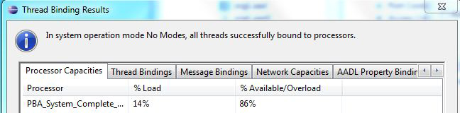
Figure 3-1. Processor Capacities of the Speed Control System Instance
Notice the information provided by the plug-in, including the actual binding for the threads determined by the plug-in (as shown in the cropped output of Figure 3-2).

Figure 3-2. Bindings from the OSATE Scheduler and Scheduling Analysis Plug-in
3.1.8. Summary
At this point, we have developed a basic architectural model of the PBA speed control system. In so doing, we have demonstrated some of the core capabilities of the AADL. For this relatively simple model, we analyzed the execution environment and made predictions of schedulability of the system. In subsequent sections, we describe additional capabilities of the AADL and discuss alternative modeling approaches that can be applied in this simple example.
3.2. Representing Code Artifacts
Within a comprehensive AADL architectural specification, source code files and related information needed for specifying and developing the software within a system are documented using standard properties. These properties capture information for documenting architectural views such as code views [Hofmeister 00] and implementation views of allocation view types [Clements 10].
In this section, we document information relating to the PBA application software contained within the process control.speed. This excludes software that may be resident in the sensors, actuators, and interface devices as well as the operating system within the processor. First, we assume the application software has been written in a programming language, such as C or Java or in a modeling language, such as Simulink. We also assume that the software has been organized using the capabilities of the source language (e.g., by organizing Java classes and methods into packages with public and private elements). In this case, we can focus on specifying a mapping of the source files into the processes and threads of the application runtime architecture. Section 3.2.1 illustrates this mapping, which can be used to generate build scripts from the AADL model. Section 3.2.2 discusses how you can map identifier names used in AADL to identifier names that are acceptable in the source language. For larger systems, we may want to reflect not only the application runtime architecture in AADL, but also the modular source code structure. Section 3.2.3 illustrates how we utilize AADL packages for that purpose.
3.2.1. Documenting Source Code and Binary Files
A modified excerpt of the PBA specification is shown in Listing 3-9. This includes a properties section within the implementation control.speed, where the property association for the property Source_Language declares that the source code language for the implementation is C. This property is of type Supported_Source_Languages, which is defined in the property set AADL_Project and has the enumeration values (Ada95, C, Simulink_6_5 are some examples). Property types and constants in the AADL_Project property set can be tailored for specific projects. For example, languages such as Java can be added to the Supported_Source_Languages property type.
Using a property association for the newly defined property Source_Language, the C language is declared as the programming language for all of the source code involved in the process control.speed. Two contained property associations for the property Source_Text identify the source and object code files for the threads speed_control_laws and scale_speed_data. Two other contained property associations for the property Source_Code_Size define the size of the compiled, linked, bound, and loaded code used in the final system.
In Listing 3-9, the data type sampled_speed_data is declared with a property association for the property Source_Data_Size. This property specifies the maximum size required for an instance of the data type. This data type is the classifier for the ports associated with the data that originates at the speed sensor.
Listing 3-9. PBA Specification with Code Properties
process implementation control.speed
subcomponents
scale_speed_data: thread read_data.speed;
speed_control_laws: thread control_laws.speed;
connections
DC1: port sensor_data -> scale_speed_data.sensor_data;
DC2: port scale_speed_data.proc_data ->
speed_control_laws.proc_data;
DC3: port speed_control_laws.cmd -> command_data;
EC1: port disengage -> speed_control_laws.disengage;
DC4: port set_speed -> speed_control_laws.set_speed;
properties
Source_Language => (C);
Source_Text => ("ControlLaws.cc", "ControlLaws.obj")
applies to speed_control_laws;
Source_Text => ("ScaleData.cc", "ScaleData.obj")
applies to scale_speed_data;
Source_Code_Size => 4 KByte applies to scale_speed_data;
Source_Code_Size => 10 KByte applies to speed_control_laws;
end control.speed;
3.2.2. Documenting Variable Names
A data port maps to a single variable in the application code. For example, the variable name for a data port can be specified using the Source_Name property. This is shown in Listing 3-10, for the in data port set_speed whose data classifier is the data type set_speed_value. The variable name for this port in the source code is SetValue.
We can use this mechanism to map data type and other component identifiers in an AADL model into the corresponding name in the source code. This is useful if the syntax of the source language allows characters in identifiers that are not allowed in AADL. We may also use this if we want to introduce more meaningful names in the AADL model for cryptic source code names.
Listing 3-10. Example of Documenting Variable Names
thread control_laws
features
proc_data: in data port;
cmd: out data port;
disengage: in event port;
set_speed: in data port set_speed_value
{Source_Name => "SetValue";};
properties
Dispatch_Protocol => Periodic;
Period => 50 ms;
end control_laws;
data set_speed_value
end set_speed_value;
3.2.3. Modeling the Source Code Structure
Source code expressed in programming languages typically consists of data types and functions. They may take the form of subprograms and functions, classes and methods, or operations on objects. These source code elements are typically organized into libraries and modular packages. Some of the library or package content is considered public (i.e., it can be used by others), whereas other parts are considered private (i.e., can only be used locally). In the case of modeling languages such as Simulink, block libraries play a similar role.
Sometimes it is desirable to represent this modular source code structure in the AADL model. We can do so by making use of the AADL package concept. For example, we can model the functions making up a Math library by placing the subprogram type declarations representing the function signatures into an AADL package together with the subprogram group declaration representing the library itself, as shown in Listing 3-11.
We can place data component types that represent classes within the same source code package, into one AADL package. We can place the data component type and the subprogram types representing the operations on the source code data type in the same package. The methods of classes can be recorded as subprogram access features of the data component type (see Section 4.2.5). Any module hierarchy in the source code can be reflected in the AADL package naming hierarchy. For more on the use of AADL packages to organize component declarations into packages, see Section 4.4.1.
Listing 3-11. Example of Modular Structure
package MathLib
public
with Base_Types;
subprogram group Math_Library
features
sqrt: provides subprogram access SquareRoot;
log: provides subprogram access;
pow: provides subprogram access;
end Math_Library;
subprogram SquareRoot
features
input: in parameter Base_Types::float;
result: out parameter Base_Types::float;
end SquareRoot;
end MathLib;
3.3. Modeling Dynamic Reconfigurations
Modes can be used to model various operational states and the dynamic reconfiguration of a system or component. In this section, we present the use of modes to represent the operation of the PBA speed control system. In this section, we develop another, slightly expanded model of the PBA speed control system.
3.3.1. Expanded PBA Model
We modify the PBA speed control model to include a display_unit. In addition, we add an out event port control_on to the interface_unit. Figure 3-3 shows the implementation of the expanded system including its subcomponents and their interconnections.

Figure 3-3. Expanded PBA Control System
The type classifiers used in the expanded PBA model are shown in Listing 3-12. In this table, we define a process type control_ex that includes the additional features required for interfacing to the display_unit and interface_unit. We could have declared this process type as an extension of the process type control, as shown in the comment. We also define the device type interface_unit as the device type interface with an additional port. Finally, we have added a new device type display_unit. The event port control_on is the trigger for a mode transition from monitoring to controlling and the event port disengage is the trigger for the reverse transition.
Listing 3-12. Type Classifiers for the Expanded PBA Model
-- Type classifiers for the expanded PBA control system model --
process control_ex
features
sensor_data: in data port;
command_data: out data port;
status: out data port; -- added port
disengage: in event port;
set_speed: in data port;
control_on: in event port; -- added port
properties
Period => 50 Ms;
end control_ex;
device interface_unit
features
disengage: out event port;
set_speed: out data port;
control_on: out event port; -- added port
end interface_unit;
device display_unit -- new device
features
status: in data port;
end display_unit;
thread monitor -- new thread
features
sensor_data: in data port;
status: out data port;
end monitor;
thread control_laws_ex
features
proc_data: in data port;
set_speed: in data port;
disengage: in event port;
control_on: in event port; -- added port
status: out data port; -- added port
cmd: out data port;
end control_laws_ex;
Listing 3-12 also includes the new thread type monitor, and the modified thread type control_laws with an extra port, now called control_laws_ex. These are the thread types of the subcomponents of the process implementation control_ex.speed. A graphical representation of the subcomponents and connections for the process implementation control_ex.speed is shown in Figure 3-4. The process speed_control, shown in Figure 3-3, is an instance of control_ex.speed.

Figure 3-4. Process Implementation control_ex.speed
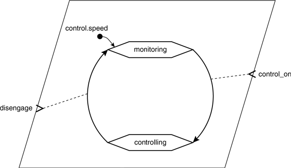
3.3.2. Specifying Modes
The textual specification for the implementation control_ex.speed is shown in Listing 3-13. In this implementation, two modes monitoring and controlling are declared in the modes section of the implementation. In the declarations for the subcomponents, the in modes declarations constrain the thread monitor to execute only in the monitoring mode and the threads scale_speed_data and speed_control_laws execute only in the controlling mode. Similarly, in the connection declarations are mode dependent such that the connections to the monitor thread are only active in the monitoring mode. The transitions between modes are triggered by the in event ports control_on and disengage. These are declared in the modes section of the implementation. If the modes are observable or are controlled from outside a component, then you may want to declare the modes in the component type.
A graphical representation for the mode transitions is shown in the lower portion of Listing 3-13. Modes are represented as dotted hexagons. The short arrow terminating at the monitoring mode denotes that the initial state is monitoring. The arrows connecting modes represent transitions. The input events are associated with the transitions that they trigger with a dotted line.
Listing 3-13. Process Implementation of control_ex.speed with Modes
process implementation control_ex.speed
subcomponents
scale_speed_data: thread read_data in modes (controlling);
speed_control_laws: thread control_laws_ex
in modes (controlling);
monitor: thread monitor in modes (monitoring);
connections
DC1: port sensor_data -> scale_speed_data.sensor_data
in modes (controlling);
DC2: port scale_speed_data.proc_data ->
speed_control_laws.proc_data in modes (controlling);
DC3: port speed_control_laws.cmd -> command_data
in modes (controlling);
DC4: port set_speed -> speed_control_laws.set_speed
in modes (controlling);
DC5: port monitor.status -> status in modes (monitoring);
DC6: port sensor_data -> monitor.sensor_data
in modes (monitoring);
DC8: port speed_control_laws.status -> status
in modes (controlling);
EC1: port disengage -> speed_control_laws.disengage
in modes (controlling);
modes
monitoring: initial mode ;
controlling: mode ;
monitoring -[ control_on ]-> controlling;
controlling -[ disengage ]-> monitoring;
end control_ex.speed;
3.4. Modeling and Analyzing Abstract Flows
One of the important capabilities of the AADL is the ability to model and analyze flow paths through a system. For example within the PBA system, it is possible to analyze the time required for a signal to travel from the interface unit, through the control system, to the throttle actuator, and result in a throttle action.
3.4.1. Specifying a Flow Model
For this section, we add flow specifications to the expanded PBA speed control system shown in Figure 3-3. We investigate a flow path (the end-to-end flow) involving a change of speed via set_speed that extends from the pilot’s interface unit to the throttle. In specifying the flow, we define each element of the flow (i.e., a flow source, flow path(s), flow sink), using on_flow as a common prefix for each flow specification name. In addition, we allocate transport latencies for each of these elements. Listing 3-14 presents an abbreviated version of the specification for the PBA speed control system that includes the requisite flow declarations.
The flow source is named on_flow_src that exits the interface unit through the port set_speed. The flow proceeds through the speed_control process via the flow path on_flow_path that enters through the port set_speed and exits through the port command_data. The flow sink occurs through the data port cmd in the throttle component. Note that a flow path can go from any kind of incoming port to a port of a different kind, for example from an event port to a data port.
Each flow specification is assigned a latency value. For example, the worst case time for the new speed to emerge from the interface unit after the pilot initiates the set_point request is 5ms. The worst case transit time through the speed_control process is 20ms and the time for the throttle to initiate an action is 8ms.7
Listing 3-14. Flow Specifications for the Expanded PBA
-- flow specifications are added to type declarations for this analysis ---
device interface_unit
features
set_speed: out data port;
disengage: out event port;
control_on: out event port;
flows
on_flow_src: flow source set_speed {latency => 5 ms .. 5 ms;};
end interface_unit;
process control_ex
features
sensor_data: in data port;
command_data: out data port;
status: out data port;
disengage: in event port;
set_speed: in data port;
control_on: in event port;
flows
on_flow_path: flow path set_speed -> command_data
{latency => 10 ms .. 20 ms;};
properties
Period => 50 Ms;
end control_ex;
device actuator
features
cmd: in data port;
BA1: requires bus access Marine.Standard;
flows
on_flow_snk: flow sink cmd {latency => 8 ms .. 8 ms;};
end actuator;
3.4.2. Specifying an End-to-End Flow
The complete path, the end-to-end flow, for this example runs from the source component interface_unit through to the component throttle. This is declared in the system implementation PBA.expanded, as shown in Listing 3-15. The declaration originates at the source component and its source flow interface_unit.on_flow_src and the connection EC4. It continues through speed_control.on_flow_path, the connection DC2, and terminates at the sink throttle.on_flow_snk. In addition, we have specified a latency of 35ms for the flow. This value is drawn from the requirements for the system.
Listing 3-15. An End-to-End Flow Declaration
system implementation PBA.expanded
subcomponents
speed_sensor: device sensor.speed;
throttle: device actuator.speed;
speed_control: process control_ex.speed;
interface_unit: device interface_unit;
display_unit: device display_unit;
connections
DC1: port speed_sensor.sensor_data ->
speed_control.sensor_data;
DC2: port speed_control.command_data -> throttle.cmd;
DC3: port interface_unit.set_speed ->
speed_control.set_speed;
EC4: port interface_unit.disengage ->
speed_control.disengage;
EC5: port interface_unit.control_on->
speed_control.control_on;
DC6: port speed_control.status -> display_unit.status;
flows
on_end_to_end: end to end flow
interface_unit.on_flow_src -> EC5 ->
speed_control.on_flow_path -> DC2 ->
throttle.on_flow_snk {Latency => 35 ms .. 35 ms;};
end PBA.expanded;
3.4.3. Analyzing a Flow
At this point, we have defined a top-level end-to-end flow, assigned an expected (required) latency value to this flow, and defined latencies for each of the elements that comprise the flow. OSATE includes a flow latency analysis tool that automatically checks to see if end-to-end latency requirements are satisfied. For example, the tool will trace the path and total the latencies for the individual elements of the flow. This total is compared to the latency expected for an end-to-end flow. Figure 3-5 presents the results of this analysis for the PBA system we have specified. The total latency for the three elements of the flow at 33ms is less than the expected 35ms.

Figure 3-5. Top Level End-to-End Flow Analysis Results
We could have manually determined, through a separate calculation, that the cumulative latency for the end-to-end flow would not violate the 35ms latency requirement. However, for very large systems, these calculations are difficult to do manually and it is difficult to ensure that latency values are correctly connected through the elements that comprise an architecture. The automated capabilities that can be included within an AADL tool facilitate easy calculation and re-calculation of these values. Moreover, having this data integral to the architecture provides a reliable way to manage the information and ensure consistency with updates to the data and the architecture.
3.5. Developing a Conceptual Model
It is possible to defer identifying the runtime nature of components until late in the development process. As noted earlier, you can do this by using system components and later manually changing the category in the relevant type, implementation, and subcomponent declarations for these components. In the next few sections, we present an alternative approach where you declare components as abstract and build an architectural component hierarchy. Then you use component extensions to create multi-view architectural representations. For example, in using the Siemens architecture approach [Hofmeister 00], you can include abstract components in a conceptual (runtime neutral) view and later extend these into runtime specific components, creating an execution view of the architecture.
3.5.1. Employing Abstract Components in a PBA Model
In declaring components for the PBA system, rather than using the device category for the pilot interface and the system category for the control components as we did in Table 3-1, we declare them as abstract. For this example, we assume there is a potential for decomposing the pilot interface into a complex interface unit. We could have made the sensor and actuator components abstract as well. However, to simplify the example and to demonstrate that you can mix abstract with runtime-specific categories, we maintain these components as devices. The declarations for this approach are shown in Table 3-2, where we have used the same partitioning and naming convention that is used in Table 3-1. Abstract components are represented graphically by dashed rectangles.
Table 3-2. Abstract Component Declarations for the PBA

A complete system implementation using abstract components is shown in Listing 3-16. We have used an enclosing system, since we plan on instantiating it. However, we could have modeled the enclosing system as abstract as well, converting it to a system model later for instantiation. We have not included the hardware components or their relevant connections in this specification. We add these later in this discussion.
Listing 3-16. Complete PBA System Using Abstract Components
system Complete
end Complete;
system implementation Complete.PBA_speed_control_ab
subcomponents
speed_sensor: device sensor.speed;
throttle: device actuator.speed;
speed_control: abstract control.speed;
interface_unit: abstract interface.pilot;
connections
DC1: port speed_sensor.sensor_data ->
speed_control.sensor_data;
DC2: port speed_control.command_data -> throttle.cmd;
DC3: port interface_unit.set_speed ->
speed_control.set_speed;
EC4: port interface_unit.disengage ->
speed_control.disengage;
end Complete.PBA_speed_control_ab;
3.5.2. Detailing Abstract Implementations
In this section, we define the implementation control.speed for the speed_control subcomponent. This is shown in Listing 3-17. We detail this component by partitioning it into two subcomponents, as we did earlier in Listing 3-3. We declare the components read_data and control as abstract and include them as abstract subcomponents in the abstract implementation control.speed. In these declarations we have not included any property associations, specifically no runtime related properties. We will defer these until we generate the execution (runtime) representation. The interfaces and connections for data and control flow are included, since this information is nominally included in a conceptual (runtime neutral) representation. As before, no data types are defined for these interfaces8.
Listing 3-17. Abstract Subcomponents for the control.speed Implementation
abstract read_data
features
sensor_data: in data port;
proc_data: out data port;
end read_data;
abstract implementation read_data.speed
end read_data.speed;
abstract control_laws
features
proc_data: in data port;
cmd: out data port;
disengage: in event port;
set_speed: in data port;
end control_laws;
abstract implementation control_laws.speed
end control_laws.speed;
abstract control
features
command_data: out data port;
sensor_data: in data port;
set_speed: in data port;
disengage: in event port;
end control;
abstract implementation control.speed
subcomponents
scale_speed_data: abstract read_data.speed;
speed_control_laws: abstract control_laws.speed;
connections
DC1: port sensor_data -> scale_speed_data.sensor_data;
DC2: port scale_speed_data.proc_data ->
speed_control_laws.proc_data;
DC3: port speed_control_laws.cmd -> command_data;
EC1: port disengage -> speed_control_laws.disengage;
DC4: port set_speed -> speed_control_laws.set_speed;
end control.speed;
3.5.3. Transforming into a Runtime Representation
We transform abstract representations into runtime representations by extending implementations. In so doing, we change the category of an implementation and its corresponding type and transform the categories of the subcomponents that reference those classifiers. We start at the lowest level of the component hierarchy, extending implementations that have subcomponents. We progress upward until we reach the complete system. For this example, we use the same runtime categories as those in the previous section (i.e., those shown in Table 3-1).
First, we extend the implementation control.speed, since it is the lowest level abstract implementation with subcomponents.9 This is shown in Listing 3-18, where a process type control_rt and a process implementation control_rt.speed are declared. The declaration of the type control_rt simply extends the type control, changing the category from abstract to process. There are no other refinements to the type. For the implementation control_rt.speed, the declaration changes the category of the implementation to process and refines (refined to) the category of both subcomponent to threads. Note that all of the characteristics (e.g., features, properties) of their ancestors are inherited by the components defined in an extension declaration (extends). Therefore, only modified elements of an implementation are included in an extension declaration of that implementation. It is not necessary to extend the type or implementation declarations for the abstract implementations read_data.speed and control_laws.speed, since there are no subcomponents in either of these implementations.10
In changing a category, it is important that the features, subcomponents, modes, properties, etc. declared for an abstract component are consistent with the semantics of the new category. For example, an abstract component with a processor subcomponent cannot be extended into a thread component.
Next, we extend the enclosing system type Complete to create Complete_rt and its implementation Complete.PBA_speed_control_ab to create Complete_rt.PBA_speed_control_ab, as shown in Listing 3-18. In the declaration of Complete_rt.PBA_speed_control_ab, we also refine the subcomponents speed_control and interface_unit, changing their category from abstract to a runtime specific category. These choices parallel the categories of the simplified model developed earlier.
Listing 3-18. Transforming the Generic PBA System into a Runtime Representation
process control_rt extends control
end control_rt;
process implementation control_rt.speed extends control.speed
subcomponents
scale_speed_data: refined to thread read_data.speed;
speed_control_laws: refined to thread control_laws.speed;
end control_rt.speed;
device interface_rt extends interface
end interface_rt;
device implementation interface_rt.pilot extends interface.pilot
end interface_rt.pilot;
system Complete_rt extends Complete
end Complete_rt;
system implementation Complete_rt.PBA_speed_control_ab extends
Complete.PBA_speed_control_ab
subcomponents
speed_control: refined to process control_rt.speed;
interface_unit: refined to device interface_rt.pilot;
end Complete_rt.PBA_speed_control_ab;
3.5.4. Adding Runtime Properties
At this point, we have refined the PBA model to include runtime components and subcomponents. However, we have not included runtime properties. For example, values for the timing properties required for a scheduling analysis are not assigned (e.g., the execution time for threads). We can do this in a number of ways. We could add local property associations to the individual abstract declarations, as shown in Listing 3-19 for the abstract types that are refined into threads. For properties that are declared as inheritable, we could modify components that are higher in the component hierarchy, relying on the inheritance of values to subcomponents (e.g., putting the values in the declarations for the abstract component type control).
Listing 3-19. Modifying Declarations with Local Property Associations
abstract read_data
features
sensor_data: in data port;
proc_data: out data port;
properties
Dispatch_Protocol => Periodic;
Compute_Execution_Time => 1 ms .. 2 ms;
Period => 50 ms;
end read_data;
abstract control_laws
features
proc_data: in data port;
cmd: out data port;
disengage: in event port;
set_speed: in data port;
properties
Dispatch_Protocol => Periodic;
Compute_Execution_Time => 3 ms .. 5 ms;
Period => 50 ms;
end Control_laws;
We could adopt a policy where we assign relevant properties by extending an abstract component (extends) and adding the property associations into the extension. This allows us to create multiple variants of the component parameterized with different property values. We can also parameterize individual subcomponents with different property values as part of a subcomponent refinement (refined to). An example of adorning the subcomponent refinements is shown in Listing 3-20.
Listing 3-20. Property Associations Adorning Subcomponent Refinements
process implementation control_rt.speed extends control.speed
subcomponents
scale_speed_data: refined to thread read_data.speed
{Dispatch_Protocol => Periodic;
Compute_Execution_Time => 1 ms .. 2 ms;
Period => 50ms;};
speed_control_laws: refined to thread control_laws.speed
{Dispatch_Protocol => Periodic;
Compute_Execution_Time => 3 ms .. 5 ms;
Period => 50ms;};
end control_rt.speed;
Another approach to centralizing property associations is to include all property declarations for the extended system in the highest system implementation declaration or for a very large system in a limited number of system implementations. To do this we use contained property associations. This is useful when different instances of the same component need to have different property values. We effectively configure an instance of the model through properties and place this configuration information (property associations) in one place instead of modifying different parts of the model. An example is shown in Listing 3-21. We assign values to the Period and Compute_Execution_Time properties for the thread subcomponents using individual property associations. We use a single property association to apply the value Periodic to the Dispatch_Protocol property for both threads.
Listing 3-21. Contained Property Associations within a System Implementation
system implementation Complete_rt.PBA_speed_control_ab extends
Complete.PBA_speed_control_ab
subcomponents
speed_control: refined to process control_rt.speed;
interface_unit: refined to device interface_rt.pilot;
properties
Period => 50ms applies to speed_control.scale_speed_data;
Compute_Execution_Time => 1 ms .. 2 ms
applies to speed_control.scale_speed_data;
Period => 50ms applies to speed_control.speed_control_laws;
Compute_Execution_Time => 3 ms .. 5 ms
applies to speed_control.speed_control_laws;
Dispatch_Protocol => Periodic
applies to speed_control.scale_speed_data,
speed_control.speed_control_laws;
end Complete_rt.PBA_speed_control_ab;
3.5.5. Completing the Specification
In order to complete the specification for the PBA system to the level of the model we developed in the previous section, we need to include hardware components, their relevant interfaces, and their interconnections. For this purpose, we simply use the updated hardware component declarations as shown in Listing 3-4.
In addition, we need to add a bus access feature to the abstract component interface.pilot. A completed PBA speed control system implementation is shown in Listing 3-22. In the table, we have highlighted the portions of Complete.PBA_speed_control_ab that were modified in the extension to Complete_rt.PBA_speed_control_ab.
By adding the hardware subcomponents into the system implementation Complete.PBA_speed_control_ab, we have a system implementation Complete_rt.PBA_speed_control_ab that is comparable to the one we generated in the previous section. That is, with this representation, we can add binding properties and conduct a scheduling analysis as we did in Section 0.
Listing 3-22. A Complete PBA System Implementation
abstract interface
features
set_speed: out data port;
disengage: out event port;
BA1: requires bus access Marine.Standard;
end interface;
device sensor
features
sensor_data: out data port;
BA1: requires bus access Marine.Standard;
end sensor;
device actuator
features
cmd: in data port;
BA1: requires bus access Marine.Standard;
end actuator;
system implementation Complete.PBA_speed_control_ab
subcomponents
speed_sensor: device sensor.speed;
throttle: device actuator.speed;
speed_control: abstract control.speed;
interface_unit: abstract interface.pilot;
RT_1GHz: processor Real_Time.one_GHz;
Standard_Marine_Bus: bus Marine.Standard;
Stand_Memory: memory RAM.Standard;
connections
DC1: port speed_sensor.sensor_data ->
speed_control.sensor_data;
DC2: port speed_control.command_data -> throttle.cmd;
DC3: port interface_unit.set_speed ->
speed_control.set_speed;
EC4: port interface_unit.disengage ->
speed_control.disengage;
BAC1: bus access Standard_Marine_Bus <-> speed_sensor.BA1;
BAC2: bus access Standard_Marine_Bus <-> RT_1GHz.BA1;
BAC3: bus access Standard_Marine_Bus <-> throttle.BA1;
BAC4: bus access Standard_Marine_Bus <-> interface_unit.BA1;
BAC5: bus access Standard_Marine_Bus <-> Stand_Memory.BA1;
end Complete.PBA_speed_control_ab;
system implementation Complete_rt.PBA_speed_control_ab extends Complete.PBA_speed_control_ab
subcomponents
speed_control: refined to process control_rt.speed;
interface_unit: refined to device interface_rt.pilot;
properties
Period => 50ms applies to speed_control.scale_speed_data;
Compute_Execution_Time => 1 ms .. 2 ms
applies to speed_control.scale_speed_data;
Period => 50ms applies to speed_control.speed_control_laws;
Compute_Execution_Time => 3 ms .. 5 ms
applies to speed_control.speed_control_laws;
Dispatch_Protocol => Periodic
applies to speed_control.scale_speed_data,
speed_control.speed_control_laws;
end Complete_rt.PBA_speed_control_ab;
3.6. Working with Component Patterns
As you use the AADL for multiple projects, you will find it convenient to reuse such things as data sensors, processors, buses, control software, and layered control architecture that have been successfully used in other projects. This is especially true if you are working in a product-line development environment.
In previous examples, we have seen how AADL can be used to define component templates (i.e., component descriptions that are completed and refined later through extension). In some cases, it is desirable to explicitly specify the placeholders (i.e., parameters) and what must be provided within a template. For example, we may have a template that is an abstract component defining a dual redundancy pattern. In that case, a user is expected to supply a single classifier that is used for both redundant instances in the pattern.
In this section, we discuss the use of parameterized component templates patterns. In so doing, we declare incomplete component types and implementations; explicitly specify what is needed to complete a pattern by declaring a prototype as a pattern parameter; and illustrate how such parameterized templates are used.
3.6.1. Component Libraries and Reference Architectures
With the AADL, it is possible to archive components and proven system solutions and reuse them through extension declarations. For this purpose, we suggest partitioning archival elements into two sets: a component library and reference architecture archive. The partitioning separates concerns such that individual, relatively simple elements are archived separately from elements involving a complex component hierarchy.
A component library is a collection of component types and component implementations with limited subcomponents that represent individual elements of a system architecture. These may be generic or runtime specific. For example, in a component library you may have a processor type marine_certified and a collection of implementations that have different processor speeds, manufacturers, and internal memory sizes. Similarly, you may have an abstract type PID_controller and its implementations that represent proportional-integral-derivative control with varying capabilities. The abstract components can be extended into runtime specific components such as a process or thread. For software components, this is the most flexible category for archiving in a library.
In your work, you may have identified a number of proven architecture solutions that have been useful. You can compile these solutions (reference architectures) into an archive that can be used in other projects. These reference architectures define common building blocks and reflect a common topology and are common throughout embedded systems development. Examples include layered control and triple modular redundant reference architectures that can be used for high dependability control avionics as well as space systems. Reference architectures can be defined at different levels of abstraction. Reference architectures can be defined using runtime-specific categories or abstract components and prototypes.
As a third approach to modeling the PBA speed control system, we use a generic component library, a reference architecture archive, prototypes, extensions, refinements, and multiple packages as demonstrations of reusing generic patterns for components and system architectures. We refine the generic components into runtime specific components in developing the PBA-specific architecture.
A library and archive can be developed without using prototypes (i.e., using only extensions and refinements). However, using prototypes makes explicit the elements (e.g., port and subcomponent classifiers) that are being refined.
3.6.2. Establishing a Component Library
Listing 3-23 shows an example generic component library that consists of two packages: interfaces_library and controller_library. In these packages, we define generic application components as abstract components. The packages are partitioned based upon a separation of concerns (e.g., the interfaces_library package has generic representations for sensors, actuators, and user interfaces). Another generic package could include only execution hardware with standard processors, memory, and bus components.
For this example, only the generic_control type has an implementation with subcomponents. In this implementation, prototypes are used in defining the subcomponents. Note that the property Prototype_Substitution_Rule is assigned the value Type_Extension. This allows within refinements, the substitution of classifiers for prototypes that are of the same type or are an extension of the original type used for the prototype. Although most of the components in this library are abstract, runtime-specific categories can be used. For example, in the abstract type declaration for generic_interface, we define a data prototype out_data that is used to define the data type in the declaration of the out data port output.
Listing 3-23. Generic Component Library
--- generic component library ---
package interfaces_library
public
abstract generic_sensor
features
output: out data port;
end generic_sensor;
abstract generic_interface
prototypes
out_data: data;
features
output: out data port out_data;
disengage: out event port;
end generic_interface;
abstract generic_actuator
features
input: in data port;
end generic_actuator;
end interfaces_library;
package controller_library
public
abstract generic_control
features
input: in data port;
output: out data port;
set_value: in data port;
disengage: in event port;
end generic_control;
abstract implementation generic_control.partitioned
prototypes
rd: abstract generic_read_data;
cl: abstract generic_control_laws;
subcomponents
r_data: abstract rd;
c_laws: abstract cl;
connections
DC1: port input -> r_data.input;
DC2: port r_data.output -> c_laws.input;
DC3: port c_laws.output-> output;
EC1: port disengage -> c_laws.disengage;
DC4: port set_value -> c_laws.set_value;
properties
Prototype_Substitution_Rule => Type_Extension;
end generic_control.partitioned;
abstract generic_read_data
features
input: in data port;
output: out data port;
end generic_read_data;
abstract implementation generic_read_data.impl
end generic_read_data.impl;
abstract generic_control_laws
features
input: in data port;
set_value: in data port;
disengage: in event port;
output: out data port;
end generic_control_laws;
abstract implementation generic_control_laws.impl
end generic_control_laws.impl;
end controller_library;
3.6.3. Defining a Reference Architecture
A sample reference architecture archive is shown in Listing 3-24, in which we have defined a generic speed control implementation Complete.basic_speed_control_ref. This implementation uses prototypes. The prototypes used here are abstract. However, prototypes can be runtime specific. In this reference architecture, we use the prototypes as classifier placeholders for the subcomponent classifiers of the implementation. For example, the prototype ssg represents the generic_sensor type that is defined in the package interfaces_library. This prototype is used in the declaration of the subcomponent ss. In using the reference architecture for the PBA, we refine the prototype into a specific runtime implementation. In this case, since we have assigned the value Type_Extension to the Prototype_Substitution_Rule property, we can substitute implementations of extensions of the component type declared in the prototype bindings.
Listing 3-24. Reference Architectures
--- reference architecture archive ---
package reference_arch
public
with interfaces_library, controller_library;
system Complete
end Complete;
system implementation Complete.basic_speed_control_ref
prototypes
ssg: abstract interfaces_library::generic_sensor;
csg: abstract controller_library::generic_control;
iug: abstract interfaces_library::generic_interface;
acg: abstract interfaces_library::generic_actuator;
subcomponents
ss: abstract ssg;
ac: abstract acg;
cs: abstract csg;
iu: abstract iug;
connections
DC1: port ss.output -> cs.input;
DC2: port cs.output -> ac.input;
DC3: port iu.output -> cs.set_value;
EC4: port iu.disengage-> cs.disengage;
properties
Prototype_Substitution_Rule => Type_Extension;
end Complete.basic_speed_control_ref;
end reference_arch;

3.6.4. Utilizing a Reference Architecture
We use the reference architecture described in the previous section to define a PBA architecture. This is shown in Listing 3-25, where the first declaration extends the abstract type Complete found in the package reference_arch. In this extension, the system category is substituted for abstract. Similarly, the abstract implementation Complete.basic_speed_control_ref is extended creating the system Complete.PBA_speed_control. In this extension, the prototypes for the subcomponents are bound to an actual classifier using a prototype binding (e.g., acg => device actuator.speed). In our example, we have fixed the classifier to be a device called actuator.speed, which will be used in the subcomponent declaration that refers to the prototype.
In the second part of Listing 3-25, each of the type and some implementation classifiers used in the prototype refinements are extended from the component library. In these extensions, PBA specific refinements can be made. For example, the data classifier speed_data is added to the out port of the sensor in the sensor type and to the input of the process type control. In addition, property associations are added in the control.speed implementation. One is the period for the threads in the process control.speed and the other is a contained property association, assigning a compute execution time to the control laws thread cl within the process control.speed.
Listing 3-25. Using a Reference Architecture
package mysystem
public
with reference_arch, interfaces_library, controller_library;
system Complete extends reference_arch::Complete
end Complete;
system implementation Complete.PBA_speed_control
extends reference_arch::Complete.basic_speed_control_ref
(acg => device actuator.speed,
ssg => device sensor.speed,
csg => process control.speed,
iug => device interface.pilot )
end Complete.PBA_speed_control;
-- defining subcomponent substitutions ---
device sensor extends interfaces_library::generic_sensor
features
output: refined to out data port speed_data;
end sensor;
data speed_data
end speed_data;
device implementation sensor.speed
end sensor.speed;
device actuator extends interfaces_library::generic_actuator
features
input: refined to in data port cmd_data;
end actuator;
data cmd_data
end cmd_data;
device implementation actuator.speed
end actuator.speed;
device interface extends interfaces_library::generic_interface
end interface;
device implementation interface.pilot
end interface.pilot;
process control extends controller_library::generic_control
features
input: refined to in data port speed_data;
end control;
process implementation control.speed extends controller_
library::generic_control.partitioned
(
rd => thread read_speed_data.impl,
cl => thread speed_control_laws.impl )
properties
Period => 20 ms;
Compute_Execution_Time => 2ms..5ms applies to cl;
end control.speed;
thread read_speed_data
extends controller_library::generic_read_data
end read_speed_data;
thread implementation read_speed_data.impl extends controller_
library::generic_read_data.impl
end read_speed_data.impl;
thread speed_control_laws
extends controller_library::generic_control_laws
end speed_control_laws;
thread implementation speed_control_laws.impl
extends controller_library::generic_control_laws.impl
end speed_control_laws.impl;
end mysystem;