Chapter 8

Times Series Regressions

Steven Hillmer

University of Kansas

It is often of interest to study the impact of a known intervention upon a second variable. Examples include the impact of an increase in tobacco taxes on teenage smoking, the impact of an environmental regulation on pollution, or the impact of an advertising campaign upon sales. Denoting the variable that is believed to be affected by the known intervention by y_t, then the relationship

can be used to not only model the impact of the intervention but also to capture the impact of other secondary factors affecting y_t. In Equation 8.1 is a row vector of independent variables including a dummy variable representing the impact of the intervention, β is a column vector of parameters, and the e_t is assumed to be independent and identically distributed random variables with mean 0 and variance σ². Thus, Equation 8.1 is the standard multiple regression model including the use of dummy variables to capture the affect of the known intervention. It is often the case that y_t is a time series, a sequence of data arranged sequentially in time. Experience with time series data suggests that the data for any time point are often correlated with its own past values, in other words, y_t is often correlated with y_t–k where k is a positive integer. This property is termed autocorrelation. When y_t is autocorrelated, it is likely that the errors e_t in Equation 8.1 will also be autocorrelated, violating one of the assumptions of the standard multiple regression model. Thus, when model 1 is used with time series data, it is prudent to be prepared for the possibility of autocorrelated error terms.

The most common approach for dealing with the possibility of autocorrelated errors is to estimate the parameters, β, assuming that the errors are uncorrelated and to perform diagnostic checks on the residuals to identify if autocorrelation is a problem. Under this approach, problems with autocorrelated errors may not be detected in diagnostic checking of the residuals. In addition, when the errors are autocorrelated, it has been established that the standard errors of the ordinary least squares estimators are incorrectly computed, which can lead to false conclusions regarding the significance of the regression coefficients (Anderson, 1971).

When dealing with time series data, a more realistic approach would be to specifically allow for autocorrelation in e_t. It is easy to specify a model for e_t which not only allows for the possibility of autocorrelation but also includes the assumption of independent errors as a special case. Under this approach the model parameters would be estimated based upon the assumption of autocorrelated errors unless there was evidence from the data to the contrary. The possibility of autocorrelated errors, e_t in Equation 8.1, can be included by assuming that e_t follows some form of common time series model.

TIME SERIES MODELS

An important set of models that describes one form of probabilistic structure for time series data is the class of stationary processes. Stationary processes follow a specific form of statistical equilibrium in which the probabilistic properties of the process are unaffected by a change in the time origin. In other words, the joint probability distribution of any set of observations e_t1, e_t2, …, e_tl is the same as the joint probability distribution of the observations e_t1+k, e_t2+k …, e_tl+k. Thus, the joint probability distribution of any set of observations is unaffected by shifting all the observations forward or backward by any k time units. This property implies that the mean and variance of a stationary process are both constant.

If the assumption of normality is made, then it follows that the probability distribution for any stationary process is completely determined once the mean, variance, and correlation coefficients between e_t and e_t+k, for each k, are specified. The mean will be denoted by µ and the variance will be denoted by . The covariance between e_t and the e_t+k, is called the autocovariance at lag k and is defined by

The autocorrelation at lag k is

Because the time series, e_t is the error in a regression model, it follows that µ = 0.

LINEAR STATIONARY MODELS

Although in theory there are many stationary time series models, experience has suggested that a relatively small set of models can be used to approximate the types of autocorrelation structure that often occurs. One class of linear stationary models are the so called autoregressive models. If a_t denotes a sequence of independent normal random variates whose mean is zero and whose variance is then the first-order autoregressive model for the time series e_t is

In Equation 8.4, ϕ₁ is a parameter that is restricted to the range –1 < ϕ₁ <1 so that the model is stationary. This model has a form like a regression equation with the lag one value of the time series in the role of the independent variable. Box, Jenkins, and Reinsel (1994) show that the variance of e_t in Equation 8.4 is and the autocorrelations follow the difference equation ρ_k = ϕ₁ρ_k–1 for all integers k ≥ 1. Because ρ_o = 1 it follows that ρ_k = (ϕ₁)^k for k ≥ 0.

A plot of the p_k versus the lag k is called the autocorrelation function of the time series. Because ρ_k = ρ_–k, the autocorrelation function is symmetric around zero and it is only necessary to plot the values of ρ_k for positive values of k. The autocorrelation function is important because, for any stationary time series, knowledge of the autocorrelations and the variance of the time series is necessary and sufficient for specification of the model associated with that time series. Thus, the autocorrelation function provides one means to specify the associated time series model. In the case of the first order autoregressive model, the autocorrelation function will exhibit a pattern of exponential decay starting with ρ₀.

A more complex stationary model is the second orderautoregressive model

The parameters ϕ₁ and ϕ₂ in Equation 8.5 must satisfy the conditions, ϕ₁ + ϕ₂ < 1, ϕ₂ – ϕ₁ < 1, and –1 < ϕ₂ < 1 for this model to be stationary. Box et al. (1994) show when e_t follows Equation 8.5, = and ρ_k follows the second order difference equation ρ_k = ϕ₁ρ_k–1 + ϕ₂ρ_k1–1 for k > 0 with starting values ρ₀ = 1 and ρ₁ = ϕ₁/(1 – ϕ₂). This implies that the autocorrelation function of Equation 8.5 will exhibit one of the following general patterns. (i) The autocorrelations remain positive while they decay to zero in an exponential type pattern. (ii) The autocorrelations alternate in sign as they decay to zero. (iii) The autocorrelations display a type of periodic behavior that is commonly characterized as a damped sine wave. The autocorrelations follow the pattern of a plot of the sine function; however, the autocorrelation also decay toward zero as the fluctuate according to a sine pattern.

A general order autoregressive model, the so called AR(p) model is

The parameters ϕ₁, ϕ₂, …, ϕ_p in Equation 8.6 must satisfy a complex set of conditions for this model to be stationary (Box et al., 1994). Although it is possible to define the general AR(p) model, in practice most time series can be appropriately modeled by a low-order AR model or one of the other models discussed later.

Although in theory the autocorrelation function of the first-order autoregressive model is different from the autocorrelation function for the second-order autoregressive model, in some cases it is difficult to tell the difference between these two autocorrelation functions from this plot. This has led to the introduction of a second plot to help distinguish between different order autoregressive models, the partial autocorrelation function. The partial autocorrelation function is based upon the fact that whereas an AR(p) model has an autocorrelation function that is infinite in extent, it is really determined by p nonzero functions of the autocorrelations. In other words, for an AR(1) model all the autocorrelations are a function of only 1 parameter, ϕ₁, and for an AR(2) model all the autocorrelations are functions of the two parameters, ϕ₁ and ϕ₂. The partial autocorrelation for lag k is equal to the correlation between e_t and e_t–k after removing the affect of the intermediate variables e_t–1, …, e_t–k+1. Box et al. (1994) show for an AR(p) model the partial autocorrelations at lags greater than p will all be zero. In other words, the partial autocorrelation function for an AR(p) model will exhibit a cutoff after lag p. This feature makes it easy to recognize the fact that an autoregressive model is associated with a given set of partial autocorrelations.

Although the class of autoregressive models are one type of model associated with stationary time series, there are a number of other stationary models that have proven useful. One class is called moving average models. The first-order moving average model is

In Equation 8.7 the a_t’s are a sequence of independent normal random variables with mean 0 and variance and Θ₁ is a parameter in the range –1 < Θ₁ < 1. Box et al. (1994) show that, when e_t follows Equation 8.7, , and ρ_k = 0 for k ≥ 2. Thus, the autocorrelation function for the first-order moving average model cuts off after lag 1. This makes it easy to recognize the first-order moving average model from its autocorrelation function. Box et al. (1994) show that the partial autocorrelation function of the first-order moving average model is dominated by exponential decay.

The second order moving average model is

with the parameters Θ₁ and Θ₂ satisfying the constraints Θ₁ + Θ₂ < 1, Θ₂ – Θ₁ < 1, and –1 < Θ₂ < 1. Box et al. (1994) show that when e_t follows Equation 8.8 , , and ρ_k = 0 for k ≥ 3. Thus, the autocorrelation function of a second-order moving average model cuts off after the second lag making it easy to recognize this model from it’s autocorrelation function.

The general order moving average model, the MA(q) model, is

As was the case in the general AR model, the parameters in Equation 8.9 must satisfy a complex set of conditions. It can be shown that the autocorrelation function of the MA(q) model cuts off after lag q, thus, the autocorrelation function is a very useful device for recognizing when a moving average model is appropriate.

The final simple stationary time series model that will be reviewed combines autoregressive and moving average model components, the ARMA(1, 1):

In this model, the parameters must satisfy the constraints –1 < ϕ₁ < 1 and –1 < Θ₁ < 1. Box et al. (1994) show that for the ARMA(1,1) model

and ρ_k = ϕ₁ρ_k–1 for k ≥ 2. Thus, the autocorrelation function of an ARMA(1,1) model will decay exponentially from the value ρ₁. It can also be shown that the partial autocorrelation function for the ARMA(1, 1) model consists of a single initial value with subsequent values characterized by a decaying exponential term such as the partial autocorrelation function of a pure MA(1) model. Thus, for the ARMA(1,1) model both the autocorrelation function and the partial autocorrelation function exhibit behavior that decays exponentially after one initial value.

All of the models that have been considered are part of the class of stationary models generally referred to as autoregressive moving average or ARMA models. Before an expression for the general ARMA model is given, it is useful to define the backshift operator B. The operator B applied to any value indexed by time (t) results in that value shifted back one unit of time, thus, Be_t = e_t–1. Furthermore, application of the operator B^k means apply the operator B k times so that B^ka_t = a_t–k. Then ϕ(B) = 1– ϕ₁B – ϕ₂B² … – ϕ_p B^p and Θ(B) = 1 – Θ₁B – Θ₂B² … – Θ_qB^q are both linear operators with ϕ(B)e_t = (1–ϕ₁B–ϕ₂B₂ … –ϕ_pB^p)e_t = e_t–ϕ₁e_t–1 – ϕ₂e_t–2 … – ϕ_pe_t–p and Θ(B)a_t = a_t – Θ₁a_t–1 – Θ₂a_t–2 … – Θ_qa_t–q. The general ARMA(p, q) model is

The parameters in the ARMA(p, q) model must be chosen so that the solutions to the equation ϕ(B) = 0 (with B treated as a variable) all have modulus greater than one and the solutions of Θ(B) = 0 also all have modulus greater than one. Notice that all the models discussed earlier were special cases of the general ARMA(p, q) model.

TIME SERIES MODELS FOR NONSTATIONARY DATA

Many times actual time series data do not appear to have one fixed mean as is required for a stationary model to be appropriate. On the other hand, these series do exhibit a kind of homogenous behavior in that, except for the fact that the level of the series is changing, each part of the series behaves very much like the other parts. Box and Jenkins (1970) were among the first authors to propose that a useful way to model this type of data is to suppose that one or more differences of the original time series may be modeled by a stationary model. This led to the autoregressive integrated moving average (ARIMA) models.

If e_t is a sequence of values, then the first difference of this sequence is e_t – e_t–1, or in terms of the backshift operator the first difference is (1 – B)e_t. The second difference of the sequence et is obtained by taking the difference of the data that has been differenced. In other words, the second difference is (1 – B)(1– B)e_t or (1 – B)² e_t. Then if the dth difference of a time series, e_t, follows an ARMA(p, q) then the time series is said to follow an ARIMA(p, d, q) model. This model is written

In practice, it is usually the case that the number of differences required to convert e_t to a stationary time series is d = 1 or 2 and the values of p and q are usually less than 2.

A STRATEGY FOR BUILDING TIME SERIES MODELS FOR OBSERVED DATA

One of the most important contributions that Box and Jenkins (1970) made was the strategy they advocated for building of a model for a given time series. Box and Jenkins began by defining a class of models that would be rich enough to characterize the behavior of a wide variety of actual time series. For the purpose of this discussion suppose that class is the ARIMA models. Box and Jenkins then suggested the three-stage model building process: (a) tentative identification of an ARIMA model, (b) estimation of the model, and (c) diagnostic checking of the model. In practice this process is not always sequential and may take several iterations as the model builder gains insight from each step in the process. A brief review of each of these model building steps follows.

MODEL IDENTIFICATION

Box et al. (1994) suggest that “identification methods are rough procedures applied to a set of data to indicate the kind of representational model that is worthy of further investigation. The specific aim here is to obtain some idea of the values of p, d, and q needed in the general ARIMA model” (p 183). The first step in identification is to determine whether or not the time series being modeled needs to be differenced in order to render it stationary and if so what particular value of d is most appropriate. Two plots that are useful in determination of the degree of differencing are a sequence plot of the time series and a plot of the autocorrelation function of the time series. A time series whose difference is stationary can be thought of as an initial value plus the sum of a finite number of terms of a series fluctuating around a fixed mean. This sum will not have a fixed level; it will either meander over time or increase over time. Thus, one of the distinguishing features of a sequence plot of a series that requires differencing is the absence of a constant level. When data exhibit a meandering level, an increasing level, or a decreasing level, the need for a difference is suggested.

The autocorrelations for a stationary time series were defined in Equation 8.3. In practice these values are unknown and need to be estimated from observed data. The most common estimator of the autocorrelations of a stationary time series are r_k = c_k/c₀ where is the estimator of the autocovariance γ_k and is the mean of the time series. The r_k values are called the sample autocorrelations, and a plot of these is called the sample autocorrelation function. Fuller (1976) has shown that r_k and c_k are consistent estimators when the data come from a stationary model and satisfy some general conditions that are met for ARMA models. Although in theory the values of ρ_k do not exist for a nonstationary time series, it is still possible to compute the values of r_k when the time series is nonstationary. Box et al. (1994) argue that a distinguishing characteristic of the sample autocorrelation function of a time series that requires differencing is that the autocorrelations fail to die out rapidly or will decrease in a linear fashion. Thus, this pattern is indicative of the need to difference the time series being modeled.

Once the value of d, the differencing, has been determined, the general appearance of the sample autocorrelation function and the sample partial autocorrelation function of the appropriately differenced data are examined to provide insight about the proper choice of the autoregressive order, p, and the moving average order, q. Pure autoregressive models are most easily identified by consideration of the sample partial autocorrelation function, which should have only “small” values after lag p. Pure moving average models are most easily identified from the sample autocorrelation function which should have only “small” values after lag q. Mixed ARMA models will have sample autocorrelation functions and sample partial autocorrelation functions that exhibit behavior that decays out rather rapidly. It is important to note that, whereas the sample autocorrelation and sample partial autocorrelation functions will exhibit behavior that is similar to their population counterparts, the sample versions are based upon estimates. Thus, in interpreting these sample functions, the individual values should be viewed in light of their associated sampling variation. In addition, it is known that large correlation can exist between neighboring values in the sample autocorrelation function; thus, individual values in these sample functions should be interpreted with care.

Although the sample autocorrelation function and sample partial autocorrelation function are very useful in identification of pure AR or MA models, in the case of some mixed models these sample functions do not provide unambiguous results. In part because of this issue, there are some other tools that have been developed to help in identification of time series models. These tools include the R array and S array approach proposed by Gray, Kelley, and McIntire (1978), the extended sample autocorrelation function of Tsay and Tiao (1984), and the use of canonical correlations used by Akaike (1976), Cooper and Wood (1982), and Tsay and Tiao (1985). Another approach that has been used in model selection is to make use of a general model selection value based upon information criteria such as AIC advocated by Akaike(1974) or BIC by Schwartz (1978). Although these information criterion approaches can be helpful, they are best used as supplementary guidelines that are part of a more detailed approach to model identification.

MODEL ESTIMATION

Once a model for a given time series has been tentatively identified, it is possible to formally estimate the parameters in this model. The most common approach to parameter estimation is to assume that the errors, a_t, have a normal distribution and to compute the maximum likelihood estimates of the parameters. It has been shown that these estimates are consistent and asymptotically normally distributed even if the distribution of the errors is not normal. Although the likelihood function is complex so it is not possible to derive closed form expressions for the maximum likelihood estimates, there are many computer programs that numerically maximize the likelihood function and compute the parameter estimates along with their standard errors. The theoretical work on parameter estimation in time series models is important in establishing properties of the estimates being computed; however, for practical purposes, what is important is an easy-to-use computer software program. The software program should have the option to maximize the exact likelihood function because it is known that maximization of approximations to the likelihood function can result in estimates of moving average parameters that are biased under some circumstances (Hillmer & Tiao, 1982).

MODEL DIAGNOSTIC CHECKING

After the parameters of a particular time series model have been estimated, it is important to examine whether or not that model adequately fits the observed data. If there is evidence of an important model inadequacy, adjustments to the estimated model should be made before conclusions are drawn or the model is used. The process of performing diagnostic checks on the fitted model is an important part of determining the usefulness of that model. “If diagnostic checks, which have been thoughtfully devised, are applied to a model fitted to a reasonably large body of data and fail to show serious discrepancies, then we shall rightly feel more comfortable about using that model” (Box et al., 1994, p. 309). On the other hand, if diagnostic checks reveal a serious problem with the model, then the model builder can be warned to modify the fitted model to address the problems.

Although there are many different types of checks that can be used, much can be learned from some relatively simple procedures. Two general methods will be reviewed: checking the autocorrelation function of the residuals from the fitted model and using a popular lack of fit test.

Most diagnostic checks for a particular fitted model are based upon the residuals from the fitted model. To illustrate how the residuals are computed, suppose the fitted model is Equation 8.10 and the parameter estimates are and then taking = 0 the residuals, can be computed recursively from the observed time series, e_t, by

The residuals for other models can be computed in a similar manner. Notice that the residuals are in effect estimates of the errors terms a_t which are assumed to be independent random variables drawn from a common normal distribution. Thus, if the model being fit is approximately correct, the residuals should exhibit properties like independent normal random variates. Conversely, if the residuals do not exhibit these properties, there is an indication of a problem with the fitted model. In particular, the sample autocorrelation function of the residuals should not have values that are larger than twice their standard errors for lags k ≥ 1.

Another common method to more formally test whether or not there are significant nonzero values in the sample autocorrelations of the residuals makes use of a whole set of these values. If r_k(â) denotes the sample autocorrelation of the residuals at lag k, then an overall test of the fitted model’s adequacy was first proposed by Box and Pierce (1970) and then modified by Ljung and Box (1978). Ljung and Box show that, if the model fitted for any ARIMA process is appropriate, then the statistic

is approximately distributed as χ² (K – p – q) where in Equation 8.14 n = T – d is the number of values available to estimate the parameters after the data have been differenced. Thus, the hypothesis that the fitted model is adequate will be rejected if for a given value of K the statistic Q exceeds (K – p – q), the value of a χ² random variable with K – p – q degrees of freedom that corresponds to a probability of a in the upper tail. If this hypothesis is rejected, efforts should be made to modify the fitted model.

Seasonal Time Series Models

It often happens that time series data exhibits a distinct “seasonal pattern with period s” when similarities in the series occur every s time intervals. For instance, many time series of monthly sales for retail establishments in the United States tend to have significantly larger values in November and December each year due to the Christmas holiday. These time series would have a period of s = 12, however, in other examples the period could be some other value. One of the important contributions of Box and Jenkins (1970) was to introduce a class of models that has over time proven to do an excellent job in the modeling of seasonal time series.

It is instructive to review the original rationale that Box and Jenkins (1970) used to develop their models for seasonal time series. Suppose a monthly time series exhibits periodic behavior with s = 12. Then the time series may be written in the form of a two-way table categorized one way by month and the other way by year. This arrangement emphasizes the fact that for a periodic time series there are two intervals of importance. It would be expected that relationships would occur between observations for the same month in successive years and between observations of successive months in the same year. This is similar to a simple two-way analysis of variance model. Box and Jenkins (1970) assume that a model that captures the relationship between the time series values of the same month in successive years is

where the seasonal frequency s = 12, D is the number of seasonal differences, and Φ(B^S) and Θ(B^S) are polynomials in the variable B^S of degrees P and Q, respectively. Equation 8.15 is the general form of the ARIMA model introduced earlier; however, the model applies to data separated by s time units. Box and Jenkins (1970) make the assumption that the same model applies to all the months and the parameters contained in each of these monthly models are approximately the same for each month.

The error components, α_t, α_t–1, …, in Equation 8.15 would not in general be uncorrelated; thus, it would be necessary to specify a model that captured the relationships between successive values in the times series. Box and Jenkins (1970) assume the model

describes the relationship between successive values. In Equation 8.16 a_t, are independent identically distributed normal random variables and ϕ(B), Θ(B) are polynomials in the variable B of degree p and q respectively. Combining Equations 8.15 and 8.16 by multiplying both sides of Equation 8.15 by ϕ(B)(1 – B)^d and substituting Equation 8.16 into the right-hand side of the resulting expression yields Box and Jenkins general multiplicative seasonal model

The process involved in building a model for a seasonal time series is similar to that discussed earlier: a model is identified, the parameters of the tentatively identified model are estimated, and diagnostic checking is carried out. The main difference for seasonal models is that the autocorrelation functions and the partial autocorrelation functions for seasonal models are more complex than those for nonseasonal models. As an example, suppose that after appropriate differencing the model for a time series was

then it can be shown that the autocorrelations for Equation 8.18 are equal to zero except ρ₀ = 1, ρ₁ = –θ₁(1 + )/(1 +)(1 + ), ρ₁₂ = –Θ₁₂(1 + )(1 + )(1 + ), and ρ₁₁ = ρ₁₃ = ρ₁ρ₁₂. Thus, the autocorrelation function has the appearance of one “nonseasonal” spike that cuts off after lag one, one “seasonal” spike at lag 12 that cuts off after one seasonal period, and the interaction between the nonseasonal and seasonal values that occur at lags 11 and 13. For models of the general multiplicative type in Equation 8.17, the autocorrelation function can often be viewed as a nonseasonal part, which follows the patterns reviewed previously combined with a seasonal part that follows the same patterns but at the seasonal periods and some additional interaction factors. Some of the patterns for the autocorrelation functions for additional seasonal models can be found in Box et al. (1994).

NONLINEAR TRANSFORMATION OF THE ORIGINAL TIME SERIES DATA

Sometimes it is the case that the variation in the time series is changing as the level of the series changes; in this case there is not only nonstationarity in the level but also in the variance. The usefulness of the general ARIMA and seasonal multiplicative ARIMA models can be expanded if the model builder is aware of the possibility of nonlinear transformation. In other words, it can happen that, whereas the Equation 8.17 may not provide an adequate representation for a given time series e_t, it may be approximately correct for some nonlinear transformation, say, ln(e_t). A simple sequence plot of the original time series can often alert the model builder to the fact that the variance is changing and a sequence plot of various nonlinear transformations can suggest the most appropriate metric of analysis. The task is to determine the metric for which the amplitude of the local variation is independent of the level of the time series. One way to define a class of nonlinear transformations and to estimate an appropriate transformation from the data is given in Box and Cox (1964).

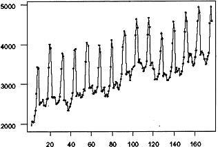
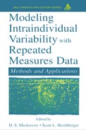
Figure 8.1: Time series plot of males aged 16 to 19.

EXAMPLE

As an illustration of modeling a seasonal time series, consider the monthly time series of employed males aged 16 to 19 in nonagricultural industries from January 1965 to August 1979. This data was modeled in Hillmer, Bell, and Tiao (1983) and is plotted in Figure 8.1. Judging from this plot, this series is seasonal, the level is changing over time, and the variability over time remains relatively stable. The failure of the sample autocorrelations, plotted in Figure 8.2, to die out rapidly and the large autocorrelations at multiples of 12 reinforce the observation that the data are nonstationary and seasonal. This suggests the need to difference the data. The sample autocorrelation function of the first difference of the data is plotted in Figure 8.3. That the autocorrelation pattern is repeated nearly exactly for every 12 lags suggests the need for a 12th difference. The sample autocorrelation function for the 12th difference of the data is plotted in Figure 8.4. The failure of the sample autocorrelations to die out rapidly suggests that both a 1st and 12th difference are necessary.

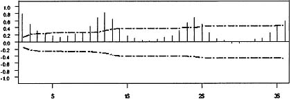
Figure 8.2: Sample autocorrelation function of males aged 16 to 19.

Figure 8.3: Sample autocorrelation function of the 1st difference of males aged 16 to 19.

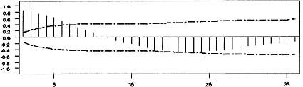
Figure 8.4: Sample autocorrelation function of the 12th difference of males.

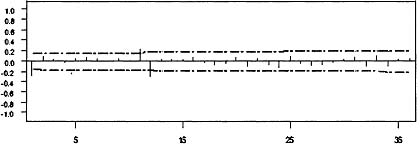
Figure 8.5: Sample autocorrelation function of the 1st and 12th differences of males.

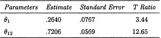
Table 8.1
Parameter Estimates for Equation 8.19

The sample autocorrelation function of the 1st and 12th differenced data is plotted in Figure 8.5. The most predominant feature of this plot is the large autocorrelations at lags 1 and 12 with another small autocorrelation at lag 11. This pattern is suggestive of the theoretical autocorrelations for Equation 8.18, thus the model

is tentatively identified as appropriate to fit this data set.

The next step in the model building process is to estimate the parameters in the model Equation 8.19 by using the SCA-PC program (Hudak & Liu, 1991), the results are given in Table 8.1. Both of the parameters appear to be statistically significant.

The sample autocorrelation function of the residuals is plotted in Figure 8.6, and a sequence plot of the residuals is plotted in Figure 8.7. These plots reveal no model inadequacies; further the Ljung-Box Q based on 36 lags equals 39.7, which is less than 48.6, the α = .05 chi-squared critical value with 34 degrees of freedom. Thus, the model in Equation 8.19 appears to be an adequate representation of this data set.

The SCA program was originally a command-driven interactive program. The SCA-PC version has a Windows interface that essentially converts the user’s responses to the Windows prompts to commands. Once the user becomes familiar with the commands, it is probably easier to type the appropriate command into the program’s command window. The commands to produce the figures and the output for the employed males example are given in Table 8.2. These commands are written based upon the assumption that the data have been read into the program and are stored in a variable named DATA.

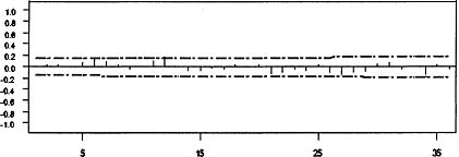
Figure 8.6: Sample autocorrelation function of residuals from Equation 8.19.

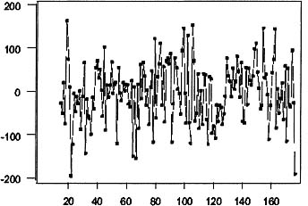
Figure 8.7: Time series plot of residuals from Equation 8.19.

Table 8.2
Commands to Produce the Output in the Employed Males Example

Command to create a time series plot of the variable DATA

GRAPH DATA. TYPE TPLOT.

Command to plot the autocorrelations of the variable DATA

GRAPH DATA. TYPE ACF.

Command to plot the partial autocorrelations of the variable

GRAPH DATA. TYPE PACF.

Command to specify the model in Equation 8.19

TSMODEL NAME MODEL1. MODEL DATA (1,12) = @ (1 - TH1∗B) (1 - TH2∗B∗∗12)NOISE.

Command to estimate the parameters for the specified model

ESTIM MODEL1. METH EXACT. HOLD RESIDUALS(RESI).

REGRESSION MODELS WITH TIME SERIES ERRORS

Now that the class of ARIMA and multiplicative ARIMA models has been reviewed, attention can return to the model in Equation 8.1 and consider the case in which e_t is not characterized by independent normal random variables but rather follows some type of ARIMA model. If the vector y′ = (y₁, …, y_T), the vector e′ = (e₁,…, e_T) and the matrix X′ = (X₁,…, X_T) then Equation 8.1 can be written as

In Equation 8.20 the covariance matrix of e, Cov(e) = V, is determined by the time series model for the error component. It is well known that the least squares estimator for the parameters in Equation 8.20 is = (X′V^–1X)^–1X′V^–1y and Cov() = (X′V^–1X)^–1. However, if a researcher proceeds as if the errors in Equation 8.20 are independent, then standard regression programs will compute the estimates = (X′X)^–1X′y so that Cov() = (X′X)^–1(X′V^–1X)(X′X). Thus, not only will the parameter estimates be incorrect, but more importantly the standard errors of the parameter estimates reported by standard computer programs and the associated t statistics used in hypothesis testing will be incorrect. Experience has suggested (see Box & Newbold, 1971) that this can cause extreme problems when the error terms in Equation 8.20 are nonstationary. Thus, it will be assumed that an observed time series y_t is related to m independent variables X_t = (x_{1, t},…, x_m,t)′ so that

with e_t following the model

The three-stage model building strategy outlined previously — identification estimation, and diagnostic checking — can be used to develop a model of the form in Equations 8.21 and 8.22 for an observed time series y_t. The main changes in this three-stage process from the steps described earlier occur at the identification stage. In practice, there often is information about independent variables that are likely to be related to y_t and that can be used to tentatively specify the regression portion of the model. As in the case of pure ARIMA models, the sample autocorrelation function and the time series plots play an important role in model identification. The first task in identification of a model for e_t is to identify the differencing needed to transform e_t to a stationary series. It is often the case (see Bell & Hillmer, 1983) that examination of the sample autocorrelation function of the original time series, y_t, is useful in determination of the degree of differencing in the noise term, e_t. This is because the impact of the nonstationarity in e_t on the computed sample autocorrelations usually dominates the impact of the regression variables. This property has been demonstrated for some particular types of regression variables by Salineas (1983). In other words, one should look for evidence of the need for differencing in the sequence plot of y_t and in the sample autocorrelation function of y_t.

After y_t (and thus e_t) have been appropriately differenced, the effect of the differenced e_t on the computed sample autocorrelations no longer dominates the effect of the differenced regression portion, β. Thus, after the appropriate degree of differencing has been determined, the sample autocorrelation function and the sample partial autocorrelation function are determined by a combination of the effect of the differenced e_t and the differenced β. To identify the model for e_t, apart from the differencing, the effects of the differenced β must be approximately removed from the differenced y_t. To achieve this the model

is fit by least squares regression. In Equation 8.23 the term (1 – B)^D(1 – B^S)^D is a row vector whose ith element is the differenced independent variable, (1 – B)^d (1 – B^S)^DX_i,t for i = 1, …, m. The sample autocorrelation function and sample partial autocorrelation function of the residuals from the model in Equation 8.23 are examined to tentatively identify the autoregressive and moving average parts of the noise model in Equation 8.22. This approach can be justified because Fuller (1976) has shown that the sample autocorrelations (and thus the sample partial autocorrelations) of the residuals from the least squares fit of Equation 8.24 differ from those of (1 – B)^d (1 – B^S)^De_t by an amount that converges in probability to zero. This procedure will be illustrated in a subsequent example.

Once the regression and time series components of the model have been tentatively identified, it is necessary to estimate the parameters. The model being estimated can be written as

Therefore, the differenced y_t values are regressed on the differenced independent variables assuming a known stationary ARMA noise model. To estimate the parameters in Equation 8.24, access to software that computes maximum likelihood estimates for this model is needed. Although there are many programs that fit ARIMA time series models, not all of these fit models of the form Equation 8.24. One of the advantages of the SCA-PC program is that it is capable of estimation of parameters in models such as Equation 8.24. After the parameters have been estimated, the residuals from the estimated model should be checked for model inadequacies in the same manner outlined previously.

Example

In Canada, retail trade stores used to be prohibited from being open on Sundays; however, this prohibition has been lifted in some provinces in recent years. For example, this prohibition was lifted in 1991 for the months of November and December in the province of New Brunswick, was further lifted to add the months of September through December in 1992, and in 1996 the month of August was included. There are several issues that may be important to policy makers as a result of the partial lifting of the prohibition of Sunday sales. In particular, there is interest in whether or not overall sales increased following the lifting of the prohibition. In addition, there is interest in whether or not there was a redistribution of sales among the days of the week to Sunday. The time series of the total department store sales in New Brunswick from 1981 to 1996 (taken from Quenneville, Cholette, & Morry, 1999) can be analyzed to provide partial answers to these types of policy interventions. The issue is to determine the degree to which these interventions affected the department store sales time series. This can be determined by building a regression model that incorporates dummy variables corresponding to the time at which the policy interventions occurred. However, because the data is a time series, it is important to specifically allow for the possibility of autocorrelated errors.

One way to access the impact of the policy change to allow stores to be open on some Sundays is to define the dummy variable I_t which takes the value 1 if t is a month including a Sunday opening and is otherwise equal to 0. I_t indicates the months in which Sunday sales were possible. Assume that the effect of stores being open on Sunday was approximately the same for each month, this effect can be estimated by including a term ηI_t in the regression portion of the model.

It is known that time series of retail sales are frequently affected by what has become known as trading day variation. Trading day variation occurs when the activity of a business varies with the days of the week so that the results for a particular month partially depends upon which days of the week occur five times. In addition, accounting and reporting practices can create trading day effects in monthly time series. For instance, stores that perform their bookkeeping activities on Fridays tend to report higher sales in months with five Fridays than in months with four Fridays. Because it is likely that the time series being modeled is affected by trading day effects, it is important to include factors in the model that will allow for this phenomena. There are a number of ways to model trading day effects by inclusion of terms in the regression portion of the model.

Let X_it, i = 1, …, 7 denote the number of Mondays, Tuesdays, and so on in month t. Then Bell and Hillmer (1983) suggest that a useful way to model the impact of trading day variation on a monthly time series is by inclusion of the regression terms where T_it = X_it – X_7t for i = 1, …,6 is the difference between the number of occurrences of each day of the week and the number of Sundays in month t and T_7t = is the length of the month t. Salineas and Hillmer (1987) show that this parameterization has less of a multicollinearity problem than a parameterization involving the variables X_it. In the expression for TD_t, the parameters β_i i = 1, …, 6 measure the differences between the Monday, Tuesday, …, Saturday effects and the average of the daily effects, which is estimated by β₇. The difference in the Sunday effect and the average of the daily effects can be shown to be . Because β₇ represents the average daily effect, which may be small in many time series, this term is often dropped from the model.

Policy makers were also interested in whether or not allowing stores to be open on Sunday during some months would shift the sales from one day of the week to Sunday. One way to answer this question is to include the terms in the regression portion of the model. The parameters δ_i i = 1, …, 6 represent the shift in impact of Monday, …, Saturday during the months when stores were open on Sunday.

It is also known that retail sales of department stores may be affected by what is known as the Easter effect, the increased buying that sometimes occurs before Easter. The placement of Easter is different from the placement of other holidays, such as Christmas, because most holidays occur in the same month each year, and thus their effect is included in the seasonal factors. In contrast, the date of Easter falls in March some months and in April other months. Bell and Hillmer (1983) propose that the effect for Easter can be modeled by a variable αE_t where the variable E_t approximates the percent increase in sales each month associated with Easter. Bell and Hillmer (1983) assume that sales uniformly increase in the 15-day period before Easter Sunday. Thus, the value of E_t is distributed between March and April proportionally to the fraction of the 15-day period falling in the respective months. The dates of Easter Sunday and the values of E_t for the years 1981 to 1996 are given in Table 8.3.

A final consideration in specifying the regression portion of a model for the department store sales is that a goods and services tax was initiated in January of 1991. This could have affected the level of sales in department stores that can be modeled by including a term λS_t in the regression model. The variable S_t has values 0 for the months before January 1991 and 1 for the months afterward. Thus, the parameter λ represents the change in the level of sales due to the institution of the tax.

In summary, a model to represent the monthly time series of department store sales in New Brunswick is

In Equation 8.25 the error term, e_t, follows some type of time series model that will be assumed to be in the ARIMA class of models. It remains to tentatively identify the model for the error term.

A good first step in identification of a model for e_t in Equation 8.25 is to examine the sequence plot of the original time series in Figure 8.8. The seasonality of the data is evident in the plot as is the generally increasing level over time. In addition, the variability of the data is changing as the level of the data becomes larger. The changing variability is a type of nonstationarity that cannot be dealt with by differencing; however, as indicated previously changing variability can often be corrected by considering a nonlinear transformation of the data. One nonlinear transformation that often stabilizes the variability is the log; thus, the natural logs of the data are plotted in Figure 8.9. The variability of the data appears to be relatively constant throughout the data; thus, the subsequent analysis will be performed on ln(y_t).

The sample autocorrelation function of ln(y_t) is plotted in Figure 8.10. The failure of the autocorrelations to die out suggests that the data need to be differenced. This is consistent with the appearance of the sequence plot in Figure 8.9. The sample autocorrelations of the first difference of ln(y_t) is plotted in Figure 8.11. The large values at lags 12, 24, and 36 together with the repeating pattern of autocorrelations every 12 lags suggests that an additional 12th difference in necessary. The sample autocorrelation of (1 – B)(1 – B¹²) ln(y_t) is plotted in Figure 8.12. The pattern is rather confusing and reflects the fact that the effect of the trading day variables, Easter, and the intervention variables in Equation 8.28 are confounded with the effect of the stationary time series model. One way to approximately eliminate the affect of the regression variables on the sample autocorrelations is to fit the regression model

and consider the sample autocorrelation function of the residuals from this model to help specify the autoregressive and moving average part the error model. The sample autocorrelation function of the residuals from this model is plotted in Figure 8.13. The most important features of this sample autocorrelation function are the large autocorrelations at lags 1 and 12. These suggest a multiplicative moving average model, (1 – θ₁)(1 – θ₁₂)a_t, for the differenced error term. This example illustrates that, when attempting to specify a model that contains both regression terms and a nonstationary ARIMA time series model, the general approach is to determine the order of differencing from the sample autocorrelation function of the original data and to determine the form of the time series model from the sample autocorrelation function of the residuals from a regression model with the variables appropriately differenced so that the error term is presumeably stationary. Thus, the final form of the tentatively identified model is

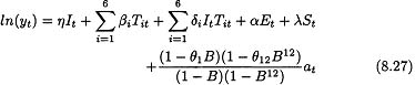
Table 8.3
Dates of Easter and E_t for the years indicated. (E_t = 0 for all other months.)

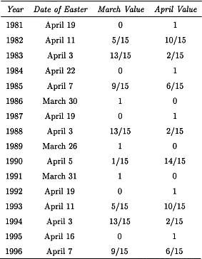
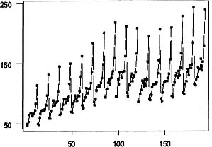
Figure 8.8: Time series plot of department store sales for New Brunswick.

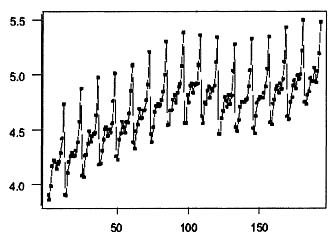
Figure 8.9: Time series plot of log department store sales for New Brunswick.

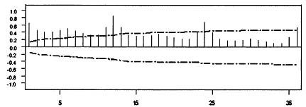
Figure 8.10: Sample autocorrelation function of log department store sales.

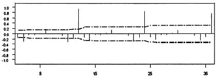
Figure 8.11: Sample autocorrelation function of the 1st difference of log sales.

Figure 8.12: Sample autocorelation function—1st and 12th differences of log sales.

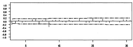
Figure 8.13: Sample autocorrelation function of the residuals from the regression model.

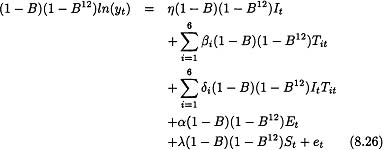
The next step in the model-building process is to estimate this model. Because the model specified in Equation 8.27 is quite complicated, it is not possible to estimate the parameters by using many of the available time series programs. One of the major advantages of the SCA-PC program is that it allows for the estimation of regression-type models that have ARIMA-type errors. The parameters are estimated by computing maximum likelihood estimators, assuming that the errors have a normal distribution. The estimators and their standard errors were computed by numerical methods in the SCA-PC program and are given in Table 8.4. There are a large number of parameters in the proposed model and, judging from Table 8.4, not all of these parameters are statistically different from zero. To eliminate those parameters whose values might as well be taken as zero, the parameters for which the absolute value of the t ratios were less than 2.00 were eliminated from the model and the reduced model was re-estimated. During this process, the parameter η was retained because part of the reason for building the model was to evaluate the impact of the known intervention, and the parameter η represents an important part of this intervention. This process of elimination of “nonsignificant” parameter estimates was repeated until all the remaining parameters (except possibly for the estimate of η) had t ratios whose absolute value was greater than 2. The parameter estimates of the resulting model are given in Table 8.5.

Before these values are interpreted, diagnostic checks should be performed on the estimated model. The sample autocorrelation function of the estimated model is plotted in Figure 8.14, because all of the values are very small, there is no evidence in this plot of any model inadequacy. The time series plot of the residuals in Figure 8.15 also suggests that there is no problem with the estimated model.

From Table 8.5, the parameters β₄, β₅, and α are clearly nonzero; this verifies that it is important to allow for trading day and Easter effects in the model. In addition, the need for differencing the data and the fact that the parameters θ₁ and θ₂ are both nonzero reflects the need to include the ARIMA time series component in the model. Finally, the fact that the parameter λ is nonzero suggests the effect of the goods and service tax that was initiated in January of 1991 was a real level change. Although these conclusions are interesting, the reason for building this model was to access the impact of on department store sales of allowing stores to be open on some Sundays. This impact is reflected by the parameters η, δ₅, and δ₆ in the model. The t ratio for the parameter η is 1.93, which suggests that the evidence that there was an increase in sales due to the opening of stores on Sunday is very slight. In contrast, the t-ratios for δ₅ and δ₆ are both large enough in magnitude to suggest that there was a shift in the impact of the trading day effects, the impact of an extra Friday was decreased, and the impact of an extra Saturday was increased. The SCA program commands to specify the model in Equation 8.26 and estimate the parameters in that model are provided in Table 8.6.

Table 8.4
Parameter Estimates for Equation 8.26 and Their Standard Errors

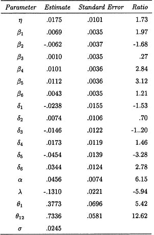
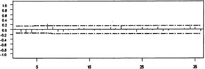
Figure 8.14: Sample autocorrelation function of the residuals from the reduced regression-time series model.

Table 8.5
Parameter Estimates for the Reduced Equation 8.26 and Their Standard Errors

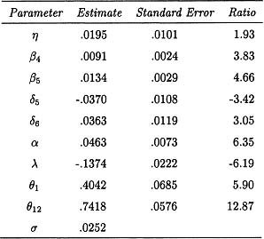
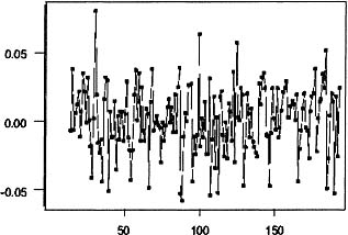
Figure 8.15: Time series plot of the residuals from the reduced model.

Table 8.6
Additional Commands to Produce the Output in the Retail Sales Example

Command to create the variable It

GENE IT. NROW 192. VALUE 0 FOR 130,1,1,0 FOR 8,1,1,1,1,@ 0 FOR 8,1,1,1,1,0 FOR 8,1,1,1,1,0 FOR 7, 1,1,1,1,1.

Command to create the variable St

GENE ST. NROW 192. 0 FOR 120, 1 FOR 72.

Command to create the trading day variables

DAYS VARI T1 TO T7. BEGIN 1981,1. END 1996,12. TRANSFORM.

Command to create the Easter variable

EASTER VARI EW. BEGIN 1981,1. END 1996,12. DURATION 15.

Command to create ItTit

TC1 = IT∗T1. TC2 = IT∗T2. continue TC6 = IT∗T6.

Command to create the natural log of the variable DATA.

NLOG = LN(DATA).

Command to specify the model in Equation 8.28

TSMODEL NAME MODEL2. MODEL NLOG(1,12) - @. (W1)IT(BINARY,1,12)+(B1)T1(B2)T2(1,12)+(B3)T3(1,12)@   +(B4)T4(1,12)+(B5)T5(1,12)+(B6)T6(1,12)+(D1)TC1(1,12)@   +(D2)TC2(1,12)+(D3)TC3(1,12)+(D4)TC4(1,12)@   +(D5)TC5(1,12)+(D6)TC6(1,12)+(W2)EW(1,12)+@   (W3)ST(BINARY,1,12)+(1 - TH1∗B)(1 - TH2∗B∗12)NOISE.

Command to estimate the parameters in the model in Equation 8.28

ESTIM MODEL2. METH EXACT. HOLD RESIDUALS(RESI).

This example illustrates that it is possible to evaluate the impact of known policy decisions in cases where the data are affected in a complex manner by external extraneous factors and when the data are autocorrelated. The example shows how to make use of external knowledge about the time series being modeled to help specify the factors that are important to include in the model beyond the hypothesized intervention. In this case these factors included trading day and Easter factors as well as a secondary intervention. The example also illustrates that an understanding of the properties of time series models also plays an important role in the model building.

REFERENCES

Akaike, H. (1976). Canonical correlation analysis of time series and the use of information criteria. In R. K. Mehra & D. C. Laniotis (Eds.), Systems identification advances and case studies (p. 27–96). New York: Academic Press.

Anderson, T. W. (1971). The statistical analysis of time series. New York: John Wiley and Sons.

Bell, W. R., & Hillmer, S. C. (1983). Modeling time series with calendar variation. Journal of the American Statistical Association, 78, 526–534.

Box, G. E. P., & Cox, D. R. (1964). An analysis of transformations. Journal of the Royal Statistical Society, 26, 211–243.

Box, G. E. P., & Jenkins, G. M. (1970). Time series analysis: Forecasting and control. San Francisco: Holden-Day.

Box, G. E. P., Jenkins, G. M., & Reinsel, G. C. (1994). Time series analysis: Forecasting and control (3rd ed.). Englewood Cliffs, NJ: Prentice Hall.

Box, G. E. P., & Newbold, P. (1971). Some comments on a paper of Coen, Gomme, and Kendall. Journal of the Royal Statistical Society, 134, 229–240.

Box, G. E. P., & Pierce, D. A. (1970). Distribution of residual autocorrelations in autoregressive-integrated moving average time series models. Journal of the American Statistical of Time Series Analysis, 65, 1509–1526.

Cooper, D. M., & Wood, E. F. (1982). Identifying multivariate time series models. Journal of Time Series Analysis, 3, 153–164.

Fuller, W. A. (1976). Introduction to statistical time series. New York: John Wiley and Sons.

Gray, H. L., Kelley, G. D., & McIntire, D. D. (1978). A new approach to arma modeling. Communications in Statistics, 7, 1–77.

Hillmer, S. C., Bell, W. R., & Tiao, G. C. (1983). Modeling considerations in the seasonal adjustment of economic time series. In A. Zellner (Ed.), Applied time series analysis of economic data. Washington, DC: U.S. Department of Commerce.

Hillmer, S. C., & Tiao, G. C. (1982). Likelihood function of stationary multiple autoregressive moving average models. Journal of the American Statistical Association, 71, 63–70.

Hudak, G., & Liu, L. (1991). Forecasting and time series analysis using the sca statistical system (Vol. 1). Oak Park, IL: Scientific Computing Associates.

Ljung, G., & Box, G. E. P. (1978). On a measure of lack of fit in time series models. Biometrika, 65, 297–303.

Quenneville, B., Cholette, P., & Morry, M. (1999). Should stores be open on Sunday? The impact of Sunday openings on the retail trade sector in New Brunswick. Journal of Official Statistics, 15, 449–463.

Salineas, T. (1983). Modeling time series with trading day variation. Unpublished doctoral dissertation, University of Kansas.

Salineas, T., & Hillmer, S. C. (1987). Multicollinearity problems in modeling time series with trading day variation. Journal of Business and Economic Statistics, 5, 431–436.

Schwartz, C. (1978). Estimating the dimension of a model. Annals of Statistics, 6, 461–464.

Tsay, R. S., & Tiao, G. C. (1984). Consistent estimates of autoregressive parameters and extended sample autocorrelation function for stationary arma models. Journal of the American Statistical Association, 79, 84–96.

Tsay, R. S., & Tiao, G. C. (1985). Use of canonical analysis in time series model identification. Biometrika, 72, 299–315.