Traditional Methods for Estimating Multilevel Models
University of Connecticut
New York University
Texas A&M University
Researchers often collect multiple observations from many individuals. For example, in research examining the relationship between stress and mood, a research participant may complete measures of both these variables every day for several weeks, and so daily measures are grouped within participants. In relationship research, a respondent may report on characteristics of his or her interactions with a number of different friends. In developmental research, individuals may be measured at many different times as they develop. In cognition research, reaction times may be observed for multiple stimuli.
These types of data structures have been analyzed using standard (ANOVA) methods for repeated measures designs. The most important limitation of the analysis of variance (ANOVA) approach is that it requires balanced data. So, in the previous examples, each person would be required to have the same number of repeated observations. For example, in the stress and mood study, everyone might have to participate for exactly 14 days, and in the relationships study each respondent might report on interactions with exactly four friends. It is often the case, however, that data structures generated by repeated observations are not balanced, either because of missing observations from some participants or, more fundamentally, because of the nature of the research design. If, for instance, researchers were interested in learning about naturally occurring interactions with friends, they might have individuals describe their interactions with each person whom they consider to be a friend. For individuals who have few friends, there would be very few observations, whereas for other individuals there would be many.
An additional factor can make the design unbalanced even if the number of observations per person is equal. For the design to be balanced, the distribution of each predictor variable must be the same for each person. So, if the predictor variable were categorical, there would need to be the same number of observations within each category for each person. If the predictor variable were continuous, then its distribution must be exactly the same for each person. The likelihood of the distribution being the same for each person is possible, but improbable. For example, in a study of stress and mood, it is unlikely that the distribution of perceived stress over the 14 days would be the same for each person in the study.
In this chapter we introduce the technique of multilevel modeling as a means of overcoming these limitations of repeated measures ANOVA. The multilevel approach, also commonly referred to as hierarchical linear modeling, provides a very general strategy for analyzing these data structures and can easily handle unbalanced designs and designs with continuous predictor variables. In introducing multilevel modeling, we focus our attention on traditional estimation procedures (ordinary least squares and weighted least squares) that, with balanced data, produce results identical to those derived from ANOVA techniques. We also introduce nontraditional estimation methods that are used more extensively in subsequent chapters.
We begin by introducing a research question on how gender of interaction partner affects interaction intimacy. We follow this by presenting an artificial, balanced data set on this topic and provide a brief overview of the standard ANOVA approach to analyzing such a data set. We then introduce a real data set in which the data are not balanced, and we consider an alternative to the ANOVA model, the multilevel model. Finally, we compare the least-squares estimation approaches described in this chapter to the maximum likelihood estimation approaches discussed in other sections of this book.
STANDARD ANOVA ANALYSIS FOR BALANCED DATAS
Consider a hypothetical Rochester Interaction Record (RIR; Reis & Wheeler, 1991) study of the effects of gender on levels of intimacy in social interaction. The RIR is a social interaction diary that requires persons to complete a set of measures, including the interaction partner’s gender and interaction intimacy, for every interaction that he or she has over a fixed interval. In our study, each of 80 subjects1 (40 of each gender) interacts with six partners, three men and three women. The study permits the investigation of the degree to which the gender of an interaction partner predicts the level of perceived intimacy in interactions with that partner. One can also test whether this relationship varies for men versus women, that is, women may have more intimate interactions with male partners, whereas men have more intimate interactions with female partners.
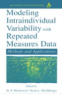
Using conventional ANOVA to analyze the data from this study would result in a source table similar to that presented in Table 1.1. In the table, partner gender is symbolized as X, subject gender is denoted as Z, and S represents subjects. Listed in the table are the sources of variance, their degrees of freedom, and the error terms for the F tests (the denominator of the F ratio) that evaluate whether each effect differs significantly from zero. The multilevel modeling terms that correspond to each effect are presented in the last column of the table. These terms are introduced later in the chapter. It is helpful to have an understanding of the different sources of variance. The between-subject variation in Table 1.1 refers to the variation in the 80 means derived by averaging each subject’s intimacy ratings over the six partners. This between-subject variation can be partitioned into three sources, the grand mean, subject gender (Z), and subject within gender (S/Z). The mean term represents how different the grand mean is from zero, and the subject gender variation measures whether men or women report more intimacy across their interactions. The third source of variation results from differences between subjects within gender. Within the group of males and females, do some people report more or less intimacy in their interactions?
The within-subject variation refers to differences among partners for each subject: Do people differ in how intimate they see their interactions with their six partners? The partner gender effect (X) refers to whether interactions with male versus female partners are more intimate. The partner gender by subject gender interaction (X by Z) refers to whether same or opposite gender interactions are seen as more intimate. The partner gender by subject interaction (X by S/Z) is the variation in the effect of gender of partner for each subject (i.e., to what degree does the mean of female partners minus the mean of male partners vary from subject to subject). Finally, there is variation due to partner (P/XS/Z), and the issue is how much the intimacy ratings of interactions with partners differ from one another controlling for partner gender. Each person reports about three male and three female partners, and this source of variance measures how much variation there is in intimacy across interactions with partners who are of the same gender. Because in this example participants interact with a given partner only once, this source of variability cannot be distinguished from other, residual sources, such as measurement error in Y. We therefore call all of the remaining variance in Y error.
Table 1.1
ANOVA Source Table for the Hypothetical Balanced Case
Within this model, there are three random effects: Subject (S/Z), Subject × Partner Gender (X by S/Z), and Error (P/XS/Z). It is possible to use the ANOVA mean squares to derive estimates for the Subject, Subject × Partner Gender, and Error variances. The subject variance, symbolized as σd2 for reasons that will become clear in the multilevel modeling section of this chapter, measures variation in average intimacy scores after controlling for both subject and partner gender. The Subject × Partner Gender variance, symbolized as σf2, measures the degree to which the effects of Partner Gender differ from subject to subject after controlling for the subject’s gender. Denoting a as the number of levels of X (a = 2 in this example) and b as the number of partners within one level of X (b = 3 in this example), then the standard ANOVA estimates of these variances are given by
As noted, an exact estimate of the partner variance cannot be obtained because it is confounded with error variance, and so we represent the combination of partner variance and error variance as σe2. Finally, although not usually estimated, we could compute the covariance between Subject and Subject × Partner Gender by computing the covariance between the mean intimacy of the subject and the difference between his or her intimacy with male and female partners. Such a covariance would represent the tendency of those who report greater levels of intimacy to have more intimate interactions with female (or male) partners. Although this covariance is hardly ever estimated within ANOVA, the method still allows for such a covariance.
The table also presents the usual mixed model error terms for each of the sources of variance. For the fixed between-subjects sources of variance, MSS/Z is the error term. To test whether there are individual differences in intimacy, MSS/Z is divided by MSP/SX/Z The error term for the fixed within-subject effects is MSX×S/Z. Finally, the error term for MSX×S/Z is MSP/SX/Z, which itself cannot be tested.
MULTILEVEL MODELS
Multilevel Data Structure
The ANOVA decomposition of variance just described only applies to the case of balanced data. For unbalanced data, a multilevel modeling approach becomes necessary. A key to understanding multilevel models is to see that these data have a hierarchical, nested structure. Although researchers typically do not think of repeated measures data as being nested, it is the case that the repeated observations are nested within persons. In hierarchically nested data with two levels, there is an upper-level unit and a lower-level unit. Independence is assumed across upper-level units but not lower-level units. For example, in the repeated measures context, person is typically the upper-level unit, and there is independence from person to person. Observation is the lower-level unit in repeated measures data, and the multiple observations derived from each person are not assumed to be independent. Predictor variables can be measured for either or both levels, but the outcome measure must be obtained for each lower-level unit. The following example should help to clarify the data structure.
Example Data Set
As an example of the basic data structure, we consider a study conducted by Kashy (1991) using the RIR. In the Kashy study, persons completed the RIR for 2 weeks. Like the previous balanced-data example, this study investigated the degree to which partner gender predicts the level of perceived intimacy in interactions with that partner and whether this relationship differs between men and women.
Because persons often interacted more than once with the same partner, we computed the mean intimacy across all interactions with each partner that is, for the purposes of this example, we created a two-level data set in which subject is the upper-level unit and partner is the lower-level unit. There are 77 subjects (51 women and 26 men) and 1,437 partners in the study. The number of partners with whom each person interacted over the data collection period ranged from 5 to 51. The average intimacy across all interactions with a particular partner is the outcome variable, and it is measured for every partner with whom the person interacted.
Partner gender, symbolized as X, is the lower-level predictor variable. Note that X can be either categorical as in the case of partner gender (X = -1 for male partners and X = 1 for female partners) or it can be continuous (e.g., the degree to which the person finds the partner to be attractive). Subject gender is the upper-level predictor variable and is denoted as Z. In repeated measures research, upper-level predictor variables may be experimentally manipulated conditions to which each subject is randomly assigned or person-level variables such as gender, a person’s extroversion, and so on. If Z were a variable such as person’s extroversion, it would be a continuous predictor variable, but because Z is categorical in the example, it is a coded variable (Z = -1 for males and Z = 1 for females). Finally, the outcome variable, average intimacy of interactions with the partner, is measured on a seven-point scale and is symbolized as Y.
Because a second example in which the X variable is continuous is helpful, we make use of the fact that Kashy (1991) also asked subjects to evaluate how physically attractive they perceived each of their interaction partners to be. Ratings of the partner’s attractiveness were centered by subtracting the grand mean across subjects from each score. (We feel that it is generally inadvisable to center X for each subject, so-called group centering.) The second example addresses whether interactions with partners who are seen as more physically attractive tend to be more intimate. We can also use subject gender as an upper-level predictor variable, which allows us to test whether the relationship between attractiveness and intimacy differs for male and female subjects.
So, in the example data set, subject is the upper-level unit, and subject gender is the upper-level predictor variable or Z. Partner is the lower-level unit and partner gender or partner’s physical attractiveness is the lower-level predictor or X. Intimacy is the outcome variable or Y, and there is an average intimacy score for each partner. The intimacy variable can range from 1 to 7, with higher scores indicating greater intimacy.
MOST BASIC APPROACH TO MULTILEVEL MODELING: ORDINARY LEAST SQUARES
Although it is certainly possible for multilevel modeling to be a challenging and complex data analytic approach, in its essence it is simple and straightforward. A separate analysis, relating the lower-level predictor, X, to the outcome measure, Y, is conducted for each upper-level unit, and then the results are averaged or aggregated across the upper-level units. In this section we introduce the ordinary least squares (OLS) approach to multilevel modeling without reference to formulas. Specific formulas describing multilevel analyses follow.
Using the partner’s physical attractiveness example, this would involve computing the relationship between a partner’s attractiveness and interaction intimacy with that partner separately for each subject. This could be done by conducting a regression analysis separately for each subject, treating partner as the unit of analysis. In the Kashy (1991) example, this would involve computing 77 separate regressions in which attractiveness is the predictor and intimacy is the criterion.
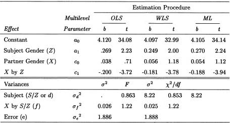
Table 1.2 presents a sample of the regression results derived by predicting average interaction intimacy with a partner using partner attractiveness as the predictor. For example, Subject 1 had an intercept of 5.40 and a slope of 1.29. The intercept indicates that Subject 1’s intimacy rating for a partner whom he perceived to be of average attractiveness was 5.40. The slope indicates that, for this subject, interactions with more attractive partners were more intimate, that is, one could predict that, for Subject 1, interactions with a partner who was seen to be 1 unit above the mean on attractiveness would receive average intimacy ratings of 6.69. Subject 4, on the other hand, had an intercept of only 2.20 and a slope of -.37. So, not only did this subject perceive his interactions with partners of average attractiveness to be relatively low in intimacy but he also reported that interactions with more attractive partners were even lower in intimacy. Note that, at this stage of the analysis, we do not pay attention to any of the statistical significance testing results. Thus, we do not examine whether each subject’s coefficients differ from zero.
The second part of the multilevel analysis is to aggregate or average the results across the upper-level units. If the sole question is whether the lower-level predictor relates to the outcome, one could simply average the regression coefficients across the upper-level units and test whether the average differs significantly from zero using a one-sample t test. For the attractiveness example, the average regression coefficient is 0.43. The test that the average coefficient is different from zero is statistically significant [t(76) = 8.48, p < .001]. This coefficient indicates that there is a significant positive relationship between partner’s attractiveness and interaction intimacy such that, on average, interactions with a partner who is one unit above the mean on attractiveness were rated as 0.43 points higher in intimacy. If meaningful, it is also possible to test whether the average intimacy ratings differ significantly from zero or some other theoretical value by averaging all of the intercepts and testing the average using a one-sample t test.
It is very important to note that the only significance tests used in multilevel modeling are conducted for the analyses that aggregate across upper-level units. One does not consider whether each of the individual regressions yields statistically significant coefficients. For example, it is normally of little value to tabulate the number of persons for whom the X variable has a significant effect on the outcome variable.
When there is a relevant upper-level predictor variable, Z, one can examine whether the coefficients derived from the separate lower-level regressions vary as a function of the upper-level variable. If Z is categorical, a t test or an ANOVA in which the slopes (or intercepts) from the lower-level regressions are treated as the outcome measure could be conducted. For example, the attractiveness-intimacy slopes for men could be contrasted with those for women using an independent groups t test. The average slope for men was M = 0.38 and for women M = 0.45. The t test that the two average slopes differ is not statistically significant, t(75) = 0.70, ns. Similarly, one could test whether the intercepts (intimacy ratings for partners of average attractiveness) differ for men and women. In the example, the average intercept for men was M = 3.78 and for women M = 4.31, t(75) = 2.19, p = .03, and so women tended to rate their interactions as more intimate than men. Finally, if Z were a continuous variable, the analysis that aggregates across the upper-level units would be a regression analysis. In fact, in most treatments of multilevel modeling, regression is the method of choice for the second step of the analysis as it can be applied to both continuous and categorical predictors.
Table 1.2
A Sample of First-Step Regression Coefficients Predicting Interaction Intimacy with Partner’s Physical Attractiveness
| Men | ||
| Subject Number | Intercept | Slope |
| 1 | 5.40 | 1.29 |
| 2 | 3.38 | .03 |
| 3 | 2.64 | .44 |
| 4 | 2.20 | -.37 |
| – | ||
| 26 | 4.17 | .48 |
| Mean | 3.78 | .38 |
| Women | ||
| Subject Number | Intercept | Slope |
| 27 | 4.07 | .16 |
| 28 | 4.10 | .45 |
| 29 | 3.88 | .98 |
| 30 | 5.53 | .32 |
| – | ||
| 77 | 4.31 | .39 |
| Mean | 4.31 | .45 |
In presenting the formulas that describe multilevel modeling, we return to the example that considers the effects of subject gender and partner gender on interaction intimacy. As we have noted, estimation in multilevel models can be thought of as a two-step procedure. In the first step, a separate regression equation, in which Y is treated as the criterion variable that is predicted by the set of X variables, is estimated for each person. In the formulas that follow, the term i represents the upper-level unit, and for the Kashy example i represents subject and takes on values from 1 to 77; j represents the lower-level unit, partner in the example, and may take on a different range of values for each upper-level unit because the data may be unbalanced. For the Kashy example, the first-step regression equation for person i is as follows:
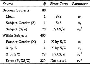
where b0i represents the intercept for intimacy for person i, and b1i represents the coefficient for the relationship between intimacy and partner gender for person i. Table 1.3 presents a subset of these coefficients for the example data set. Given the way partner gender, or X, has been coded (-1, 1), the slope and the intercept are interpreted as follows:
b0i: the average mean intimacy across both male and female partners
b1i: the difference between mean intimacy with females and mean intimacy with males divided by two
Table 1.3
Predicting Interaction Intimacy with Partner’s Gender: Regression Coefficients, Number of Partners, and Variance in Partner Gender
Note: Gender of partner is coded 1 = female, -1 = male.
Consider the values in Table 1.3 for Subject 1. The intercept, b0i, indicates that across all of his partners this individual rated his interactions to be 5.35 on the intimacy measure. The slope, b1i, indicates that this person rated his interactions with female partners to be 1.52 (0.76 X 2) points higher in intimacy than his interactions with male partners.
For the second-step analysis, the regression coefficients from the first step (see Equation 1.3) are assumed to be a function of a person-level predictor variable Z:
There are two second-step regression equations, the first of which treats the first-step intercepts as a function of the Z variable and the second of which treats the first-step regression coefficients as a function of Z. In general, if there are p variables of type X and q of type Z, there would be p + 1 second-step regressions each with q predictors and an intercept. There are then a total of p(q + 1) second-step parameters. The parameters in Equations 1.4 and 1.5 estimate the following effects:
a0: the average response on Y for persons scoring zero on both X and Z
a1: the effect of Z on the average response on Y
c0: the effect of X on Y for persons scoring zero on Z
c1: the effect of Z on the effect of X on Y
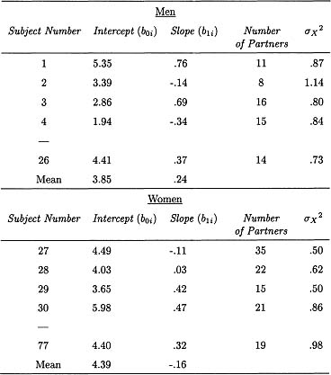
Table 1.4 presents the interpretation of the four parameters for the example. For the intercepts (b0i, a0, and c0) to be interpretable, both X and Z must be scaled so that either zero is meaningful or the mean of the variable is subtracted from each score (i.e., the X and Z variables are centered). In the example used here, X and Z (partner gender and gender of the respondent, respectively) are both effect-coded (-1, 1) categorical variables. Zero can be thought of as an “average” across males and females. The estimates of these four parameters for the Kashy example data set are presented in the OLS section of Table 1.5.
As was the case in the ANOVA discussion for balanced data, there are three random effects in the multilevel models. First, there is the error component, eij, in the lower-level or first-step regressions (see Equation 1.3). This error component represents variation in responses across the lower-level units after controlling for the effects of the lower-level predictor variable, and its variance can be represented as ![]() . In the example, this component represents variation in intimacy across partners who are of the same gender (it is the partner variance plus error variance that was discussed in the ANOVA section). There are also random effects in each of the two second-step regression equations. In Equation 1.4, the random effect is di and it represents variation in the intercepts that is not explained by Z. Note that di, in this context is parallel to MSS/Z within the balanced repeated measures ANOVA context, as shown in Equation 1.1. The variance in di is a combination of
. In the example, this component represents variation in intimacy across partners who are of the same gender (it is the partner variance plus error variance that was discussed in the ANOVA section). There are also random effects in each of the two second-step regression equations. In Equation 1.4, the random effect is di and it represents variation in the intercepts that is not explained by Z. Note that di, in this context is parallel to MSS/Z within the balanced repeated measures ANOVA context, as shown in Equation 1.1. The variance in di is a combination of ![]() , which was previously referred to as Subject variance, and
, which was previously referred to as Subject variance, and ![]() . Finally, in Equation 1.5, the random effect is fi, and represents variation in the gender of partner effect. Note that fi here is parallel to MSXbyS/Z within the repeated measures ANOVA context, as shown in Equation 1.2. The variance in fi, is a combination of
. Finally, in Equation 1.5, the random effect is fi, and represents variation in the gender of partner effect. Note that fi here is parallel to MSXbyS/Z within the repeated measures ANOVA context, as shown in Equation 1.2. The variance in fi, is a combination of ![]() , which was previously referred to as the Subject by Gender of Partner variance, and
, which was previously referred to as the Subject by Gender of Partner variance, and ![]() . A description of these variances for the example is given in Table 1.4.
. A description of these variances for the example is given in Table 1.4.
Table 1.4
Definition of Effects and Variance Components for the Kashy Gender of Subject by Gender of Partner Example
| Effect Estimate | Multilevel Parameter | Definition of Effect |
| Constant | a0 | Typical level of intimacy across all subjects and partners |
| Subject Gender (Z) | a1 | Degree to which females see their interactions as more intimate than males |
| Partner Gender (X) | c0 | Degree to which interactions with female partners are seen as more intimate than those with male partners |
| X by Z | c1 | Degree to which the partnergender effect is different for male and female subjects |
| Variance | ||
| Subject | σd2 | Individual differences in the typical intimacy of a subject’s interactions, controlling for partner and subject gender |
| X by Subject | σf2 | Individual differences in the effect of partner gender, controlling for subject gender |
| Error | Wihin-subject variation in interaction intimacy, controlling for partner gender (includes error variance) | |
Table 1.5
Estimates and Tests of Coefficients and Variance Components for the Kashy Gender of Subject of Partner Example
Note. OLS, WLS, and MLS estimates were obtained using the SAS REG procedure, the SAS GLM procedure, and HLM, respectively.
Recall that it was possible to obtain estimates of ![]() and
and ![]() for balanced designs by combining means squares. As can be seen in Equations 1.1 and 1.2, in the balanced case the formulas involve a difference in mean squares divided by a constant. In the unbalanced case (especially when there is a continuous X), this constant term becomes quite complicated. Although we believe a solution is possible, so far as we know none currently exists.
for balanced designs by combining means squares. As can be seen in Equations 1.1 and 1.2, in the balanced case the formulas involve a difference in mean squares divided by a constant. In the unbalanced case (especially when there is a continuous X), this constant term becomes quite complicated. Although we believe a solution is possible, so far as we know none currently exists.
The multilevel model, with its multistep regression approach, seems radically different from the ANOVA model. However, as we have pointed out in both the text and Table 1.1, the seven parameters of this multilevel model correspond directly to the seven mean squares of the ANOVA model for balanced data. Thus, the multilevel model provides a more general and more flexible approach to analyzing repeated measures data than that given by ANOVA, and OLS provides a straightforward way of estimating such models.
Computer Applications of Multilevel Models with OLS Estimation
One of the major advantages of using the OLS approach with multilevel data is that, with some work, virtually any statistical computer package can be used to analyze the data. The simplest approach, although relatively tedious, is to compute separate regressions for each upper-level unit (each person in the case of repeated measures data). In SAS, separate regressions can be performed using a “BY” statement. If PERSON is a variable that identifies each upper-level unit, the SAS code for the first-step regressions could be:
PROC REG
MODEL Y = X
BY PERSON
Then a new data set that contains the values for b0i and b1i for each upper-level unit, along with any Z variables that are of interest, would be entered into the computer. The OLS approach is certainly easier, however, if the computer package that performs the first-step regressions can be used to create automatically a data set that contains the first-step regression estimates. Although this can be done within SAS using the OUTEST = data set name COVOUT options for PROC REG, it can be rather challenging because SAS creates the output data set in matrix form. Regardless of how the data set is created, the coefficients in it serve as outcome measures in the second-step regressions.
Complications in Estimation with Unbalanced Data
The OLS approach to multilevel modeling allows researchers to analyze unbalanced data that cannot be handled by ANOVA. As we have noted, there are two major reasons that data are not balanced. First, persons may have different numbers of observations. This is the case in Kashy data set where the number of partners varies from 5 to 51. Second, even if the number of observations were the same, the distribution of X might vary by person. In the example, X is partner gender, and the distribution of X does indeed vary from person to person and so the variance of X differs (see Table 1.3). As noted earlier, data are unbalanced if either the number of observations per person is unequal or the distribution of the X variables differs by person. Note that a study might be designed to be balanced, but one missing observation makes the data set unbalanced.
MULTILEVEL ESTIMATION METHODS THAT WEIGHT THE SECOND-STEP REGRESSIONS
The OLS approach does not take into account an important ramification of unbalanced data: The first-step regression estimates from subjects who supply many observations, or who vary more on X, are likely in principle to be more precise than those from subjects who supply relatively few observations or who vary little on X. A solution to this problem is to weight the second-step analyses that aggregate over subjects by some estimate of the precision of the first-step coefficients. How best to derive the weights that are applied to the second-step analyses is a major question in multilevel modeling, and there are two strategies that are used: weighted least squares (WLS) and maximum likelihood (ML). Because the ML approach is treated in detail in other chapters in the volume, we focus most of our attention on the WLS solution. However, we later compare WLS, as well as OLS, with ML.
Multilevel Modeling with Weighted Least Squares
Expanding the multilevel model from an OLS solution to a WLS solution is relatively straightforward. As in OLS, in the WLS approach a separate analysis is conducted for each upper-level unit. This first-step analysis is identical to that used in OLS, as given in Equation 1.3. The second-step analysis also involves estimating Equations 1.4 and 1.5. However, in the WLS solution, Equations 1.4 and 1.5 are estimated using weights that represent the precision of the first-step regression results.
The key issue then is how to compute the weights. In WLS, the weights are the sums of squares for X or SSi (Kenny et al., 1998). This weight is a function of the two factors that cause data to be unbalanced: The number of lower-level units sampled (partners in the example), and the variance of X (partner gender in the example).
Multilevel Modeling with Maximum Likelihood
The major difference between ML and WLS solutions to multilevel modeling is how the weights are computed. The ML weights are a function of the standard errors and the variance of the term being estimated (see chapter 5 for greater detail). For example, the weight given to a particular boi is a function of its standard error and the variance of di. ML weighting is statistically more efficient than WLS weighting, but it is computationally more intensive. There is usually no closed form solution for the estimate, that is, there is no formula that is used to estimate the parameter. Estimates are obtained by iteration and the estimates that minimize a statistical criterion are chosen. In ML estimation, the first and second-step regressions are estimated simultaneously. Several specialized stand-alone computer programs have been written that use ML to derive estimates for multilevel data: HLM/2L and HLM/3L (Bryk, Raudenbush, & Congdon, 1994), MIXREG (Hedeker, 1993), MLn (Goldstein, Rasbash, & Yang, 1994), and MLwiN (Goldstein et al., 1998). Within major statistical packages, SAS’s PROC MIXED and BMDP’s 5V are available.
ESTIMATION OF WLS USING STANDARD COMPUTER PROGRAMS
The estimation of separate regression equations is awkward and computationally inefficient. Moreover, this approach does not allow the researcher to specify that the X effect is the same across the upper-level units. It is possible to perform multilevel analyses that yield results identical to those estimated using the “separate regressions” WLS approach but that are more flexible and less awkward. This estimation approach treats the lower level or observation as the unit of analysis but still accounts for the random effects of the upper level. We illustrate the analysis using SAS’s GLM procedure as an example. The analysis could be accomplished within most general linear model programs. We use SAS because it does not require that the user create dummy variables, but other statistical packages could be used. The WLS analysis that we describe requires that a series of three regression models be run, and then the multilevel parameters and tests are constructed from the results of these three models.
Lower-level units are treated as the unit of analysis. In other words, each observation is a separate data record. Each record has four variables: the lower-level predictor variable X, the upper-level predictor variable Z, the outcome variable Y, and a categorical variable, called PERSON in the example that follows, which identifies each individual or upper-level unit in the sample. In the first run or Model 1 the setup is:
PROC GLM
CLASS PERSON
MODEL Y = Z PERSON X Z∗X PERSON∗X
The mean square error from the model is the pooled error variance or ![]() . Also, the F tests (using SAS’s Type III Sum of Squares) for both PERSON and PERSON by X are the WLS tests of the variance of the intercepts
. Also, the F tests (using SAS’s Type III Sum of Squares) for both PERSON and PERSON by X are the WLS tests of the variance of the intercepts ![]() and the variance of the slopes
and the variance of the slopes ![]() , respectively. Note that this model supplies only the tests of the intercept and slope variances. The other tests are not WLS tests and should be ignored2.
, respectively. Note that this model supplies only the tests of the intercept and slope variances. The other tests are not WLS tests and should be ignored2.
Model 2 is the same as Model 1 but the PERSON by X term is dropped:
PROC GLM
CLASS PERSON
MODEL Y = Z PERSON X Z∗X/SOLUTION
This model gives the proper estimates for main effect of X (c0) and the Z by X interaction (c1) (see Equation 1.5). The SOLUTION option in the MODEL statement enables these estimates to be viewed. Mean squares for these terms are tested using the PERSON by X mean square (SAS’s Type III) from Model 1 as the error term. If there are multiple X variables, Model 2 must be re-estimated dropping each PERSON by X interaction singly.
Finally, Model 3 is the same as Model 1 except the PERSON term is dropped:
PROC GLM
CLASS PERSON
MODEL Y = Z X Z∗X PERSON∗X/SOLUTION INT
The term INT is added so that the intercept can be viewed. This model gives the estimates of the Z effect (a1) and the overall intercept (a0) from Equation 1.4. The mean squares for these terms are tested using the PERSON Mean Square (Type III) from Model 1.
If there were two X variables, X1 and X2, then Model 2 would be estimated twice. In one instance, the PERSON by X1 term would be dropped; however, the effects of the both X1 and X2 would remain in the equation as well as the PERSON by X2 interaction. In other instance, the PERSON by X2 term would be dropped; however, the effects of the both X1 and X2 would remain in the equation as well as the PERSON by X1 interaction. If there were more than one Z variable, they could all be tested using a single Model 3.
The results from the tests of the variances of Model 1 have important consequences for the subsequent tests. If there were evidence that an effect (e.g., f) does not significantly vary across upper-level units and so ![]() is not statistically significant, Model 1 should be re-estimated dropping that term. In this case, instead of using that variance as an error term for other terms in Model 2, those terms can be tested directly within Model 1 using the conventional Model 1 error term. So if
is not statistically significant, Model 1 should be re-estimated dropping that term. In this case, instead of using that variance as an error term for other terms in Model 2, those terms can be tested directly within Model 1 using the conventional Model 1 error term. So if ![]() is not included in the model, c0 and c1 would be tested using the
is not included in the model, c0 and c1 would be tested using the ![]() . Rarely, if ever, is the variance of the intercepts not statistically significant. However, if there was no intercept variance, a parallel procedure would be used to test a0 and a1.
. Rarely, if ever, is the variance of the intercepts not statistically significant. However, if there was no intercept variance, a parallel procedure would be used to test a0 and a1.
Table 1.5 presents the OLS, WLS, and ML results for the Kashy data set. The OLS and WLS estimates were obtained from SAS using the methods described previously. The ML estimates were obtained using the HLM program (Bryk et al., 1994).
Model 1 is estimated first to determine whether there is significant variance in the intercepts and slopes across persons. There is statistically significant evidence of variance in the intercepts [F(75, 1283) = 8.22, p < .001]; however, there is not evidence that the slopes significantly vary [F(75, 1283) = 1.22, p = .10). We adopt the conservative approach and treat the slopes as if they differed.
We see that the intercept is near the scale midpoint of four. Because effect coding is used, effects for respondent gender, partner gender, and their interaction must be doubled to obtain the difference between males and females. We see from the subject gender effect that females say that their interactions are more intimate than reported by males by about half a scale point. The partner effect indicates that interactions with females are perceived as one tenth of a point more intimate than interactions with males. Finally, the interaction coefficient indicates that opposite-gender interactions are more intimate than same-gender interactions.
One feature to note in Table 1.5 is the general similarity of the estimates. This illustrates how WLS and even OLS can be used to approximate the more complicated ML estimates. Of course, this is one example and there must be cases in which ML is dramatically different from the least-squares estimators. We discuss this issue further in the following section.
COMPARISON BETWEEN METHODS
In this section we consider the limitations and advantages of OLS, WLS, and ML estimation. The topics that we consider are between and within slopes, scale invariance, estimation of variances and covariances, statistical efficiency, and generality.
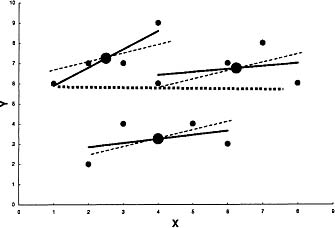
Figure 1.1: Individual within (solid line), pooled within (small dashed), and between line (large dashed line).
Between and Within Slopes
The coefficient b1i measures the effect of X on Y for person i. In essence, OLS and WLS average these b1i values to obtain the effect of X on Y. However, there is another way to measure the effect of X on Y. We can compute the mean X and mean Y for each person, and then regress mean Y on mean X (again weighting in the statistically optimal way) treating person as the unit of analysis. So for the example, we could measure the effect having more female partners on the respondent’s overall level of intimacy. We denote this effect as bB and the average of the b1i or within-subject coefficients as bW.
Figure 1.1 illustrates these two different regression coefficients. There are three persons, each with four observations denoted by the small-filled circles. We have fitted a slope for each person, designated by a solid line. We can pool these three slopes across persons to compute a common, pooled within-person slope or bW. This slope is shown in the figure as the dashed line that we fitted for each person. The figure also shows the three points through which bB is fitted (the large-filled circles). The slope bB is fitted through these points and is shown by the large dashed line.
There are then two estimates of the effect of X on Y: bW and bB. In essence, bW is an average of the persons’ slopes, and bB is the slope computed from the person means. For the Kashy data set, we estimated these two slopes for the effect of partner gender on perceived intimacy. The value for bW is 0.056, indicating that interactions with female partners are seen as more intimate. However, the value for bB is negative being - 0.217. This indicates that people who have relatively more female partners viewed their interactions as less intimate. (The coefficient is not statistically significant.)
The ML estimate, as we have described it, of the effect of X on Y is a compromise of the two slopes of bW and bB whereas the WLS and OLS estimates use only a version of bW. Note that in Table 1.5 the ML estimate for this effect (X) is somewhat lower than the WLS estimate because ML uses the negative between slope. In our experience, these two slopes are typically different, and, as the example shows, sometimes they even have different signs. So, it is a mistake to assume without even testing that the two slopes are the same. The prudent course of action is to compute both slopes and evaluate empirically whether they are equal. If different, in most applications we feel that bW is the more appropriate.
To estimate both slopes the following must be done: create an additional predictor variable that is the mean of the Xs for each person (Bryk & Raudenbush, 1992). Thus, there are two X predictors of Y: Xij and the mean X. The slope for Xij estimates bW and the slope for mean X estimates bB. Alternatively, the X variables can be “group-centered” by removing the subject mean for each variable (for more on centering in multilevel models see Kreft, de Leeuw, & Aiken, 1995).
We should note that, in the balanced case, mean X does not vary, and so bW can be estimated but bB is not identified. Perhaps, the balanced case has misled us into thinking that there is just one X slope (bW) when in fact in the unbalanced case there are almost always two (that may or may not be equal).
Scale Invariance
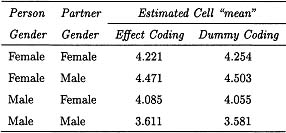
There is a serious limitation to WLS estimation that is not present in either ML or OLS. Second-stage estimates using WLS estimation of intercepts are not scale invariant, that is, if an X variable were transformed by adding a constant to it, the WLS second-step solution for the intercepts cannot ordinarily be transformed back into the original solution. The reason for this lack of invariance is that the weights used in the step-two equations differ after transformation. The standard error for the intercept increases as the zero point is farther from the mean. Because of the differential weighting of the intercepts, estimates of cell “means,” using the intercepts, will not be the same.
To illustrate this problem using the sample data set, we recoded the data using dummy coding (males = 0, females = 1) instead of effect coding for the both person and partner gender variables. Table 1.6 presents the estimated cell means for the four conditions. We see that there is a difference between the predicted “means” and so the coding system matters.
Because ML estimates the weights simultaneously, it does not to have this problem.3 Because OLS does not weight at all, OLS does not have this problem. Thus, this serious problem applies only to WLS. One simple solution to the problem is to always center the X variables using the grand mean. It is fairly standard practice to do this anyway.
Table 1.6
Estimated Cell “Means” for the Four Conditions Using WLS
Estimation of Variances and Covariances
One major advantage of ML is that it directly provides estimates of variances and covariances. A procedure for obtaining WLS estimates of variance has been developed (Kashy, 1991), but it is very complicated. We know of no appropriate method for estimating covariances within WLS. Because slopes and intercepts are typically weighted differently, it is unclear how to weight each person’s estimates to form a covariance.
It seems logically possible that estimates of both variance and covariance could be developed within OLS. However, we know of no such estimates. If OLS were to be used more in estimation in multilevel models, it would be of value to determine these estimators.
ML has the strong advantage of providing estimates of these variances and covariances. Unfortunately, we should note that all too often these terms are largely ignored in the analysis. Most of the focus is on the fixed effects. Very often the variances and covariances are as important as the fixed effects. Knowing that X has the same effect on Y for all subjects (i.e., ![]() is zero) can often be a very interesting result because it implies that effect of X on Y is not moderated by individual differences.
is zero) can often be a very interesting result because it implies that effect of X on Y is not moderated by individual differences.
If we assume that the statistical model is correct, OLS is the least efficient, WLS the next, and ML the most. The complex weighting of ML creates this advantage. We wonder, however, whether this advantage may at times be more apparent than real. Consider the Kashy study. For both ML and WLS, why should people who have more partners count more than those with fewer? Statistically, more is better, but that may not be the case in all repeated measures studies.
Perhaps, if there is a disparity in the number of observations per person, the researcher might want to test if number of observations (perhaps log transformed) is a moderating variable, that is, does the effect of X on Y increase or decrease when there are more observations? Number of observations would then become a Z variable entered in the second-step equations. We estimated such a model with the Kashy data and did not find evidence for moderation, but we did find a trend that persons with more interaction partners reported lower levels of intimacy.
Generality
There are several complications of the model that we might want to consider. First, the outcome variable, Y, may be discrete, not continuous. For instance, in prevention studies, the outcome might be whether the person has a deviant status or not. Second, X or Y may be latent variables. In social-interaction diary studies, there may be several outcomes (intimacy, disclosure, and satisfaction) that measure the construct of relationship quality. It may make sense to treat them as indicators of a latent variable. Third, we have assumed that after removing the effect of the Xs the errors are independent. However, the error may be correlated across time, perhaps with autoregressive structure. Fourth, the distribution of errors may have some other distribution besides normal (e.g., log normal). Typically, behavioral counts are highly skewed and so are not normal. Fifth, the variance in the errors may vary by person. Some people may be inherently more predictable than others.
Increasingly, ML programs allow for these and other complications. However, it would be difficult if not impossible to add these complications to a least-squares estimation solution. Thus, ML estimation is much more flexible than least-squares estimation.
SUMMARY
Multilevel modeling holds a great deal of potential as a basic data analytic approach for repeated measures data. An important choice that researchers will have to make is which multilevel estimation technique to use. Although statistical considerations suggest that ML is the best estimation technique to use because it provides easy estimates of variance and covariance components, is flexible, and provides estimates that are scale invariant, there are times that OLS might also be very useful. We should note that ML estimation is iterative, and sometimes there can be a failure to converge on a solution. Moreover, ML estimation, as conventionally applied, pools the between and within slopes without evaluating their equality. Therefore, when ML is used in an unsophisticated manner, it is possible to end up confounding what may be conceptually very different effects.
OLS approaches are familiar and easy to apply, and results generated by OLS generally agree with those produced by ML. WLS has some advantages over OLS. Its estimates are more efficient and estimates of variance components are possible. However, it suffers from the problem that the intercept estimates are not scale invariant.
Notably, if the data set is balanced or very near balanced, there is only a trivial difference between the different techniques. ML estimation still has the advantage that variance components can always be estimated, but, if the design is perfectly balanced, the variance components can be estimated and tested using least squares. A major advantage of both OLS and WLS solutions is that they can be accomplished by using conventional software (although SAS’s PROC MIXED is available for ML). Thus, a researcher can use conventional software to estimate the multilevel model.
WLS and OLS may serve as a bridge in helping researchers make the transition from simple ANOVA estimation to multilevel model estimation. It may also be a relatively easy way to estimate multilevel models without the difficulties of convergence and iteration. Finally, and most importantly, it can provide a way for researchers who are not confident that they have successfully estimated a multilevel model using new software to verify that they have correctly implemented their model. We have generations of researchers who are comfortable with ANOVA and who have difficulty working with multilevel regression models. These people can estimate models using a WLS approach that approximates the more appropriate ML.
Regardless how the researcher estimates a multilevel model, we strongly urge the careful probing of the solution. Even the use of standard ANOVA is complicated, and errors of interpretation are all too easy to make. Researchers need to convince themselves that the analysis is correct by trying out alternative estimation methods (some of which may be suboptimal), plotting raw data, and creating artificial data and seeing if the analysis technique recovers the model’s structure. We worry that, in the rush to use these exciting and extraordinarily useful methods, some researchers may not understand what they are doing and they will fail to make discoveries that they could have made using much simpler techniques.
Supported in part by grants to the first author from the National Science Foundation (DBS-9307949) and the National Institute of Mental Health (R01-MH51964). Questions to the first author can be sent by email to [email protected].
REFERENCES
Bryk, A. S., & Raudenbush, S. W. (1992). Hierarchical linear models: Applications and data analysis methods. Newbury Park, CA: Sage.
Bryk, A. S., Raudenbush, S. W., & Congdon, R. T. (1994). Hierarchical linear modeling with the HLM/3L programs. Chicago, IL: Scientific Software International.
Goldstein, H., Rasbash, J., Plewis, I., Draper, D., Browne, W., Yang, M., Woodhouse, G., & Healy, M. (1998). A user’s guide to MLwiN. Institute of Education, University of London. (http://www.ioe.ac.uk/multilevel/)
Goldstein, H., Rasbash, J., & Yang, M. (1994). MLN: User’s guide for version 2.3. London: Institute of Education, University of London.
Hedeker, D. (1993). MIXREG. A FORTRAN program for mixed-effects linear regression models. Chicago, IL: University of Illinois.
Kashy, D. A. (1991). Levels of analysis of social interaction diaries: Separating the effects of person, partner, day, and interaction. Unpublished doctoral dissertation, University of Connecticut, Storrs, CT.
Kenny, D. A., Kashy, D. A., & Bolger, N. (1998). Data analysis in social psychology. In D. Gilbert, S. Fiske, & G. Lindsey (Eds.), The handbook of social psychology (Vol. 1, 4 ed., p. 233–265). Boston, MA: McGraw Hill.
Kreft, I. G. G., de Leeuw, J., & Aiken, L. S. (1995). The effect of different forms of centering in hierarchical linear models. Multivariate Behavioral Research, 30, 1–21.
Reis, H. T., & Wheeler, L. (1991). Studying social interaction with the rochester interaction record. In M. P. Zanna (Ed.), Advances in experimental social psychology (Vol. 24, p. 269–318). San Diego, CA: Academic Press.
__________________________________
1We use subject to refer to the research participants so that subjects (S) can easily be distinguished from partners (P) in our notation.
2The reader should be warned that, in the output, the Z effect has zero degrees of freedom. This should be ignored.
3However, if the same equation were estimated twice (e.g., an X variable is present in one equation and dropped in the other), ML is likely to weight the effect differently in the two equations. This differential weighting creates difficulties in the decomposition of indirect effects in mediation.