5
Modeling a DLE Perceived as a Complex System
We have just explained in the preceding chapter that we are choosing to study latest generation DLEs, referring to the theory of complex system modelling, because we perceive them as complex phenomena (for example, an MOOC). Now, let us look at the different stages of this model and its instrumentation.
According to the systemic modeling theory, modeling a complex system first consists of modeling a synchronic action system1 (that functions), a diachronic action system2 (transforming while functioning), a teleological action system (having a purpose, a goal) and recursive action system (automation) in an active environment. Systemic modeling also passes by respect of a conjunctive logic which aims to join and not separate the active environment and project (or teleology) concepts on the one hand, and those of synchronic functioning (doing) and diachronic transformation (becoming) on the other.
The cybernetic procedure characterizes the conjunction of the first two concepts; the structuralist procedure, the conjunction of the last two. The general system (GS) concept results in the conjunction of these two modeling procedure support concepts, namely the cybernetic and structuralist procedures.
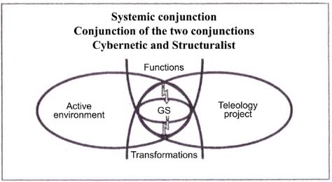
Systemic conjunction therefore proposes “to keep inseparable ‘the operation and transformation of a phenomenon, the active environments’ in which it is carried and ‘projects’ against which it is identifiable” [LEM 99, p. 40].
“Any complex system can therefore be represented by ‘a system of multiple actions’ or by ‘a process’ that can be a tangle of processes. This can be represented by the designation of identifiable ‘functions’ that it exercises or may exercise” [LEM 99, p. 48].
Systemic modeling (SM) does not begin to represent things, objects, individuals, bodies, as is done in analytical modeling (AM), but an action (characterized by a process) that can be a tangle of actions (or a complex of actions) that one will systematically represent by the black box (or a symbolic processor)3 that accounts for this action or a complex of actions. This is the basic concept of systemic modeling (SM)4 other than from what “the system performs”, in other words, operations and transformations or ensured operations or those to be ensured. However, “identifying preconceived N processors and input and output couples by which one characterizes them is not given by the problem that the modeler considers” [LEM 99, p. 54]. Therefore, starting from the projects that we will address, this will be the model design process. The latter will be built by successive iterations “between projects and symbolic representations that the modeler constructs” [LEM 99, p. 54].
5.1. Finalized and recursive processes in an active environment
5.1.1. Identifiable finalized processes (functions)
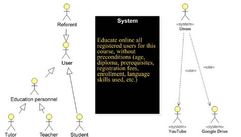
Initially, the modeler has a basic perception of the world to model. This first stage of the systemic modeling of complexity corresponds to the first level of an archetype model for the connection of a nine-level complex system as described in section 5.1.2.2. Its perception, at first syncretic, of the system or phenomenon to model does not allow it to see the details. It then determines its outline, its borders5 with the outside world and examines its global function that it will later set out. The purpose of the project will be described in its dynamic dimension. Without going into the details of this description that strongly depends on the type of project to model6, remember that the main function of a DLE is to allow the learner to acquire knowledge and develop skills through the use of a digital environment. Variations to this general description are justified from the moment the DLE is considered or not considered by the modeler as a new generation DLE. If so, it must assume its complexity and describe what characterizes its function. In the case of an MOOC, for example, modeling will be necessarily different from that of a traditional distance education mechanism. For example, the project would be to “educate online all those registered for this course, without preconditions (age, diploma, pre-requisites, registration fees, enrollment, language skills used, etc.)”. A first representation could be shown in Figure 5.3.

Figure 5.3. DLE represented by a black box
It is at this stage that the modeler can register the system (the process) in its environment; the project becomes identifiable and differentiable from its environment. The latter is also composed of different actors7.
“An actor represents a coherent set of roles played by the entities that interact with the system. These entities can be human users or other subsystems” [MAM 11, p. 8].
Among these actors, we will examine the primary actors from the secondary actors.
The primary actors act directly on the system. In the case of a DLE, this mainly relates to the learner subjects, teachers, tutors, training managers, computer scientists, programmers, designers and developers. They all need to use the system, the first group to learn, the second to teach and the last to maintain the system in good working order.
Secondary actors do not have a direct use of the DLE. They can nevertheless be called upon or consulted by the primary actors in the system, either to exchange information or to meet specific needs. These are usually actors outside the system considered as service providers (for example, Moodle in the first MOOC EFAN8) or simply partners (for example, those of Coursera9). YouTube and Dailymotion are other examples of secondary actors, both offering hosting of videos to MOOCs. This is precisely the case of Dailymotion who hosts FUN (France Université Numérique) MOOC videos.
Some actors are of the “human” type, and others not. To differentiate between them, some modeling languages represent human actors by stick figures. Their respective roles in the system are indicated in Figure 5.4.

Figure 5.4. A representation of a human type actor
To represent a “non-human” type actor, the modeler can either choose a representation among those proposed by current modeling languages or choose its own representation. In the first case, the representations may vary. This goes from the stick figure non-human actor with a large black bar on its head to the non-human actor represented by the same stick figure, but with an indication of the <<system>> stereotype, through to a simple box with an indication of the <<system>> stereotype (see Figure 5.5).

Figure 5.5. A representation of a human type actor
Continuing with the example of an MOOC for illustration purposes, the latter would be made up of human and non-human actors who interact with the system. DLE users who need this environment to learn would naturally be a part of the human actors. Video webhosts belong to the category of non-human actors. The black box becomes the opportunity to learn for human users.
The description of nested processes or complex actions ensues from this activity, which will gradually fill the black box, which represents both the system and its overall project.
“with the families of projects, we will associate subsystem hypotheses that one seeks to connect... referring to the overall project of the modelling system (and not to the hypothetical nature of things). Then departing from the levels, we will attempt to put them together in a processor system, as a composer deliberately looking to compose a musical system with the help of a symbolic representation system. Modeling a complex system will organize a series of iterations between the projects and symbolic representations that the modeler has contracted” [LEM 99, p. 54].
This procedure is what Le Moigne calls systemography10.
This set of multiple actions or processes identified by the modeler can take place inside of a concept map, created in order to represent them (see Figures 5.7–5.11). It is advisable to clarify the perceived traits of the phenomenon to model everything by completing the map.
“It should be noted that these taxonomies are based on the needs of a specific world. They are often limited, considering real-life experiences of the subject(s)-explorer(s). They are derived from customized investigations of the world to model; then, they are consolidated by the consensus approach undertaken by the project team, when there is one, and mediators, bearers of scholarly knowledge. The team agrees to share objects, terms and definitions to come to a relevant judgment in relation to the components of the world which should be taken into account throughout the project to complete. This worldly description is first based on the intersubjectivity of the people involved: they support their judgment through the use of real-life experiences, or they justify appropriateness taking position in a subjective way. This is the description of a complex system and layout of its components in various models that will result from this cognitive activity” [LEM 08, p. 75].

Figure 5.7. An example of a blank process system concept map
These representations include structural matrices, arrangements, tree diagrams, conceptual maps or any other development that can be used in the representation of projects, actions, complex actions, functions (processors) or simply relationships that unite them.
To facilitate the representation of these processors, we agree to indicate them by “Pr”, the processor symbolizing the “black box”, and by “ti”, the period during which the values of its inputs and outputs are assigned. The processes characterizing the active phenomenon are now perceived in their actions (acting within the system).
Peraya [PER 03], Meunier and Peraya [MEU 04], Charlier Deschryver and Peraya [CHA 06] were interested in the “approach by constituent functions of any publicized educational environment” without (to our knowledge) having an explicit reference to the theory of complex system modeling. Today, the analysis framework relative to these constituent functions of any publicized educational environment constitutes a frame of reference.
Based on different taxonomies that scientific literature proposes11, these authors retain eight functions, namely (1) awareness or highlighting of “signs of the presence of distance actors” [WEI 03, JAC 06]; (2) social interaction which includes what is conventionally referred to as collaboration, communication and exchanges; (3) information defined within the meaning of the provision of resources or objects; (4) production (individual or collective); (5) management and planning (activities and actors); (6) support and assistance; (7) emergence and systematization of meta-reflexive activity; (8) and “auto and hetero-evaluation” [PER 08, p. 20].
Each of these functions has a relationship with the others, and among all of them, it happens to be that some of them are perceived as primary by modelers compared to others. For example, the function of “information management” appeared central to Peraya and Bonfils [PER 14, p. 13] in a study conducted on PLEs (personal learning environments). In this study, “subjects tested instantiated five of the eight constituent functions of any publicized educational environment: it concerned these functions : (1) sharing ongoing issues and resources, (2) management information, (3). awareness, remote social presence, embodied by notifications, (4) production of written and multimedia documents and (5) communication and interaction. Each of these functions are associated with one or more specific mechanisms” [PER 14, p. 13]. These functions recognized and explained by the modelers are examples of this first modeling stage that we are presenting here. They take place in a concept map built for this purpose (see Figure 5.8).

Figure 5.8. Modeling of group working environments [PER 14, p. 26]
5.1.2. Recursive processes
We have seen that the recognition of the terms and legends inhabiting the conceptual map of a system and serving to name each of the perceived phenomenon traits to model is done by using successive iterations. The modeler (or project team12 responsible for modeling) iteratively completes this map by crossing, one by one, the functional levels of an archetype model (nine levels) that we described in section 5.1.2.4. “The argument is to be considered a sort of progressive complexification of systemic modeling” [PER 14, p. 58]. Adjustments will be made by successive iterations in order to minimize as much as possible the distance between a representation built by the modeler and the representation of users13. The architect who designs a project for a client always proposes several versions of the plans before producing a final version (the one accepted by the customer). This is also true when a business manager conducts the analysis of its production system. The first alarming piece of information concerning its assembly line is not sufficient to declare the system as failed. The latter will be subjected to further tests which, iteratively, will confirm a possible recurring malfunction. In our case, the iterative approach is similar to a process that consists of going back and forth between the construction of the model and the information gradually provided by the project actors and information and amassed by the modeler. The latter thus builds a system representation ever closer to reality. Better organized and more complete versions gradually appear. As the philosopher and logician Jean Ladrière14 once said in 1974: “It’s a teleology that is built. There is no teleology established in advance, there is a process of learning through which a tentative first approach manages to draw more and more precisely its own path. Internal process of auto-finalization”.
In this regard, we have already noted that the approaches and latest generation modeling languages such as object approach or the corresponding UML are organized around basic principles of which the first is based on an iterative and incremental approach.
5.1.3. Representation of the processes and functional levels of the system
In some cases, the modeler can see that the number of processors quickly increases. This should lead him to groups of processors in families or categories of processors. They can be classified, interrelated and prioritized in a “parents” and “children” tree diagram. This is a way of proceeding, starting from recognition of actions or complex of actions (processors), allowing the construction of more or less specific categories used to group these processors into parts, taking into account their properties or attributes. “We can then differentiate the system into many subsystems or levels, each level capable of being modeled by its network and interpreted relatively independently as soon as the interlevel coupling interrelationships have been carefully identified” [PER 14, p. 54].
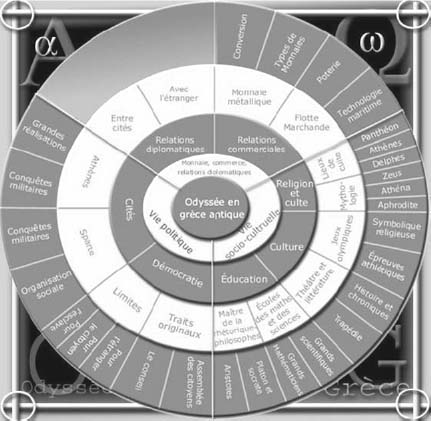
Figure 5.9. A conceptual map produced by a French project team discussing the elements of Ancient Greek society [LEM 08, p. 94]
For example, if we can recognize an essential DLE function in distance tutoring, we can also admit that it corresponds to the combination of a number of functions: technological support, content expertise, methodological advice, animation, assessment [DEV 10, p. 3].
We have seen that graph theory makes a range of useful representations available to systemic modeling. Gilles Lemire, with whom we have worked concerning issues in system modeling since the early 2000s, offers the following conceptual map in his book Modélisation et construction des mondes de connaissances [Modeling and construction of knowledge worlds]15. The classification of components explains “institutions of ancient Greece (political, cultural and economic life); this remains an interesting illustration of this process for the development of a world of knowledge to construct” [LEM 08, p. 93].
“In topological terms, the core of the conceptual map brings identification of the ‘world’ in which self-construction is undertaken; the first circle is fragmented in view of large classes, and the one that follows according to the number of subclasses. Specificity levels can stretch to terms representing concrete beings placed in the space that surrounds the last circle” [LEM 08, p. 93].
Other functional representations are possible. Two examples are shown in Figures 5.10 and 5.11, respectively.
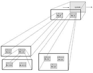
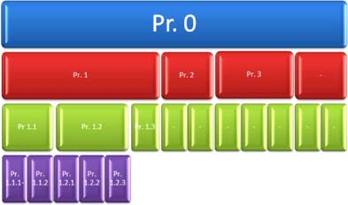
Figure 5.11. Example 2 of a hierarchical representation. For a color version of this figure, see www.iste.co.uk/trestini/learning.zip
5.1.4. The eight constituent functions of a DLE applied to systemic modeling
It is also possible to represent the general process of a DLE using, for example, the eight functions identified16 by Peraya [PER 03], Meunier and Peraya [MEU 04], Charlier et al. [CHA 06] as well as Peraya D., Charlier B., and Deschryver N., [PER 08, p. 20]. The exercise simply consists of completing the blank conceptual maps of the above representations. As Le Moigne recalls:
“The General System is somehow a matrix whose modeler will establish, by molding a preconceived footprint (‘framing’ phase: general-modeling system) isomorphy. It then has a blank systemic model, without a legend. The ‘development’ phase will precisely involve writing captions, in other words establishing correspondences between the features of this systemic model and perceived or conceived traits of the phenomenon to model. The model ‘with the legend’ will thus be systemic (it is molded on the preconceived system)”17 [LEM 99, p. 41].
Figure 5.12 shows cases where these functions are applied to the diagram in Figure 5.8.

Figure 5.12. The eight constituent functions of any publicized educational environment [PER 08, p. 20] written at the heart of the conceptual map of the general process of a DLE
But it would also be possible to integrate these eight functions (or a part of them) into any other graphic representation (Figure 5.13, for example), based on the models we have just proposed in Figures 5.10 or 5.11, for example.

Figure 5.13. An application of the constituent functions in previous models. For a color version of this figure, see www.iste.co.uk/trestini/learning.zip
We saw in sections 3.4 and 5.2.5 that there are complex system modeling languages that offer a range of symbolic representations, which are used to model these processes effectively. They are generally available from a library specific to the software used. Figures 5.14 and 5.15 give representations borrowed from UML (Unified Modeling Language), mainly resulting from “object-oriented” modeling (OMT) by Rumbaugh et al. [RUM 95]. We have also justified this choice in section 5.2.5. In this example, we recognize the eight processors18 referred to earlier in Figure 5.12:
- – awareness;
- – support and tutoring;
- – management and planning, etc.

Figure 5.14. Eight processors in UML (or packages). For a color version of this figure, see www.iste.co.uk/trestini/learning.zip

Figure 5.15. An extract from the support and tutoring use case built for Project Management MOOCs (see full diagram in section 6.1.1). For a color version of this figure, see www.iste.co.uk/trestini/learning.zip
NOTE.– Here, we will only provide incomplete views to illustrate our point. They will be fully developed in Chapter 6.
The box surrounding these processors corresponds to the black box (in blue), or the encompassing processor, in other words, the system (Figure 5.14). Figure 5.15 represents the “children” processors of the supporting and tutoring processor as an example.
In UML language, the diagram in Figure 5.14 represents the functional decomposition of the system processors also called “packages” in this language (another meaning for the same word!)19. This diagram can also indicate the actors involved in each of the packages. The diagram in Figure 5.15 represents children processors (also known as “use case” in this language), functions more specifically necessary to users. In UML, it is possible to make a use case for a DLE chart as a whole or for each package. Here, the use case bears the “support and tutoring” processor.
5.2. Synchronic processes (the system performs)
Processors registered in the heart of the concept map20 will now be operated in turn, taking into account the actions they produce (explaining how the input values (inputs)21 of each processor are transformed to become output values (outputs)). To model an active environment involves modeling the activity exercised by the fulfillment of actions, transactions and interactions.
This step corresponds to the second level of archetype model (nine levels) complexification.
“This identifiable phenomenon is perceived actively: it is perceived because it is presumed to ‘do’ something. In terms of modeling techniques, we go from the ‘ticker’ symbolizing a closed set to the ‘black box’ symbolizing an active processor” [LEM 99, p. 59].
We immediately add a level of additional complexity that the designer is able to perceive and represent simultaneously: the self-regulation of the identified processes. This is located on the third level of archetype model complexification.
“To be effectively identifiable, the phenomenon must be perceived by some form of consistency or stability. Its behavior, because it is perceived, is presumed to be ‘regulated’: we don’t model the chaos or the erraticism! In other words, the modeler assumes the emergence of some internal regulation mechanisms” [LEM 99, p. 59].
To highlight the presence of actions and counter-reactions, in other words, interrelationships of actions (network and feedback), we suggest indicating their active presence (section 5.2.1) by recording their origin and their destination in a structural matrix. To translate the presence of regulation within a system at a given time (the system that performs and seems regulated), we will draw up the inventory of input and output values for each of them (section 5.2.2).
Then, to “account for the growing complexification of this regulation” [LEM 99, p. 60], placed at the third level of archetype model complexification, we propose the construction of a data flow diagram (section 5.2.3) with the ability to highlight the information produced by the system, but also its intermediary forms and the systems of symbols, providing intermediation and regulation, similar to the way “of presumed electric impulse that through nerves or a circuit, transmit regulation instructions, reflecting changes in the system’s state” [LEM 99, p. 60]. We will also show that the digital learning environment that we model is also able to inquire about its own behavior.
In the section that follows, we will address fourth level of archetype model complexification, not only statically (the system “performs”) but according to its dynamic component (the system “becomes”). We will describe the typical phases of the processes (scenarios), highlighting the events that activate the actions (section 5.3.1). The traces left by these events will be helpful in developing the state diagrams of the processes involved.
We will finally offer a description of each of these functions (processor) (section 5.3.4) before specifically focusing on a DLE’s ability to process information, decide its own behavior and remember information (see section 5.4). This progressive complexification of systemic modeling corresponds, respectively, to the fifth and sixth levels of an archetype model.
5.2.1. Identifying the active presence of interrelationships
Let us start by outlining a simple method allowing the identification of the active presence of interrelationships which includes feedback, also known as “recycling”.
The structural matrix built for a similar purpose by Le Moigne [LEM 99, p. 50] is resumed at good cost in the modeling approach that we propose.
“The complexification of the system modeled will be made by an interrelation of the previously identified N processors by the composed functions that each provides. It is said that there is interrelation between two Pi and Pj processors when an output (or an output vector component) Pi processor is an input to the Pj processor. IR interrelation (Pi, Pj is then enabled”.
“All combinations of possible interrelationships among N processors can be represented using the structural matrix of the system (representation that can be refined by the creation of the N2 matrices from PiPj coupling in the case where the Pi outputs can be the inputs of several different Pj, Pk, Pl processors...)”.
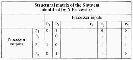
Figure 5.16. A matrix of possible interrelationships between N processors [LEM 99, p. 50]
“The presence of a 1 in the O/P Pi, I/P Pj box means that the Pi, Pj interrelation is enabled; the presence of a zero means that this interrelationship is not enabled, and possibly that it is prohibited. This Boolean structural matrix allows the economic presentation of several interesting characteristics of a complex system” [LEM 99, p. 50].
In addition to the interest that this simple representation contains when viewing the system interrelations formally and quickly, it also has the advantage of benefiting from its integrating effect to “show new behaviors, rarely predictable by linear composition22” [LEM 99, p. 50], which we have seen in section 5.2.6, allowing a connection with “our” prospective projects put into perspective. But it is true that in practice, modeling a complex system is rarely done by starting with the construction of the structural matrix because the preconceived identification of N processors and input-output pairs by which they are characterized... is not given by the problem that the modeler considers [LEM 99, p. 54]. Therefore, it will rather be starting from known system projects that SM will propose to initiate in the model’s design process.
5.2.2. Establishing an input and output value inventory for each process
From a methodological point of view, and in order to facilitate the construction of an input and output inventory and the recognition of functional dependencies that follow, we propose adopting a method inspired by “object-oriented” (OMT) 23 modeling developed by Rumbaugh et al. [RUM 95]. In this particular IT modeling paradigm, an object is nothing other than a simple constituent of the system. This clarification is important because it keeps us safe from a situation that could become sensitive to SM choice (vs. AM), a choice extensively explained in the preceding chapters. With this IT paradigm, the object represents a concept, idea or any entity from the physical world and not only a static grantor or a body of the system. And if the object can represent a concept, a process can be an object in this sense since it is itself a concept24. Moreover, object-oriented methods also address the issue of modeling complex phenomena perceived as complex by their dynamic and functional aspects, derived from modeling models of the same name to which we will have the opportunity to revisit.
In an object-oriented approach and in order to identify the input and output values, one usually represents the process by “a flowchart” (or a data flow diagram) which allows the output values from input values to be obtained. For a determined process state, it is a matter of specifying its activity and determining the organization of operations that define it, explaining data flow that circulate during these operations.
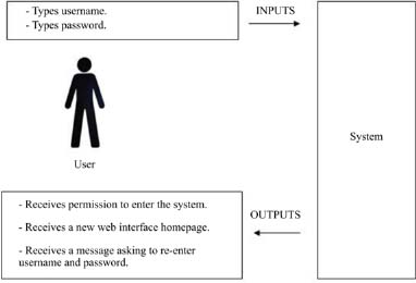
Figure 5.17. The identification of input and output values for a given system state
The identification of input and output values occurs at the time of a fine analysis of the constituent action sequences of any process. It is a task that consists of identifying the list of information carrier events that are then transformed into data transmitted to the system or issued by the system. This information transports input values, such as, for example, the identification of a user wishing to connect to his DLE (an MOOC, for example). This alphanumeric information becomes an input value that tells the system that the user is registered (or not) to the course and that the latter seeks approval to integrate the activities to which he is registered. Screens of different types or input (or output) windows (input mask) of information can result from this approach and take place on the screen depending on the processing that the system will perform from this information. Here, the general activity is learning, and the goal is to enter the system. The system interface is to allow the user entry by referring relevant information based on the information received. For example, the system can accept to host the user if the data provided is consistent with the data previously established by a “decision-making system”, which will itself have provided this data to a “memory system” providing a storage function of information. Input values may be the identifier and the password, for example, and the output values the message “password or identification invalid: try again” or even “a new web interface home page”.
5.2.3. Representing data flow and functional dependencies between processes
On the fourth level of archetype model complexification, “everything happens as if the system has endogenously produced intermediary forms, information, symbol systems, which would provide regulation intermediation” [LEM 99 p. 60]. To account for the growing complexity of this regulation, it seems reasonable to propose sketching a data flow diagram. From the approach of object-oriented modeling (OMT), this diagram graphically represents the flow of data between the various processes in the system. “It allows the determination of its borders, the area of study, the system processes, processing (activities) and gives a concrete view of the system to build”25 or analyze. It is also used to show functional dependencies.
It should also be noted that this diagram “is interested in processing data without regard to sequencing ‘decisions’ or the structure of objects” [RUM 95, p. 178]. Its interest is to show how the output values are obtained from the input values, or how these values are processed, and how the system will behave.
We have said that this is also the moment when new behaviors within the system can emerge because of this connecting of processors.

Figure 5.18. The highest level flow diagram of an MOOC interface
In practice, this diagram is usually built in layers which successively refine non-trivial processing: any non-trivial processing must be described by a sub-diagram. “The highest level layer may consist of a single treatment or may be a treatment to collect entries, another to deal with data, and one to produce the outputs” [RUM 95, p. 180].
Figure 5.18 shows the highest level data flow diagram of a MOOC interface, taken as an example, and considered here as a latest generation DLE (the legend is in Appendix 1).
Figure 5.19 develops the process, producing the outputs of Figure 5.18 and gives the example of a non-trivial data flow sub-diagram of the general diagram. In the same way, this sub-diagram can be developed in other sub-diagrams. The processor showing the forum will certainly give rise to the development of another data flow diagram and so on.
In diagrams, “features are identified by the verbs used to account for the events to update. They become the opportunity for a relationship of association between entities: each time, this creates a ‘functional dependency’” [LEM 08, p. 151]. Relationship cardinality characterizes the relationship between an entity and the relationship. Functional dependency is said to be strong for a cardinality (1,1) and weak for cardinality (0,1) [LEM 08, p. 152].
“Cardinalities allow for the characterization of links that exist between an entity and the relationship to which it is connected. Relationship cardinality consists of a couple with a minimal and maximum point, an interval in which the cardinality of an entity can take its value: (i) the minimum point (usually 0 or 1) describes the minimum number that entity can participate in a relationship; (ii) the maximum point (usually 1 or n) describes the maximum number of times that an entity can participate in a relationship. A 1.n cardinality means that each entity belonging to an entity class participates at least once in the relationship. A 0.n cardinality means that each entity belonging to an entity class does not necessarily participate in the relationship” [LEM 08, p. 152].
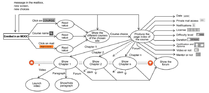
Figure 5.19. A processor data flow diagram "producing” MOOC OpenClassrooms “outputs”
Also note that the represented DLE equally contains objects used as information storage (Figure 5.18). This is the case here in the registered database that most notably stores their usernames and their passwords. “Data reservoirs differ from data flow or processing by the fact that the entry of a value does not result in an immediate exit, but rather this value is reserved for future use”. This memory system will be discussed on the sixth level of archetype model complexification
Furthermore, although the data flow diagram (Figure 5.20) shows “all the possible ways of processing” [LEM 08, p. 181], they are usually waived decisions. Like the memory system, the decision-making system will be studied in detail later and especially when we get to the fifth level of archetype model complexification. Decision functions, such as, for example, those who verify a username or a password, obviously influence the result. Some data values can exclude certain intended actions or affect the outcome of a decision.
“Decisions do not directly affect the data flow model since this model shows all the possible ways of processing. It may however be useful to enter the decision functions in the data flow model to the extent that they can be complex functions of the input values. Decision functions can be represented in a data flow diagram, but they are indicated by dotted outgoing arrows. These functions are only indications on the data flow diagram; their result only affects the flow control and not the values themselves” [RUM 95, p. 181].
Here is an example:
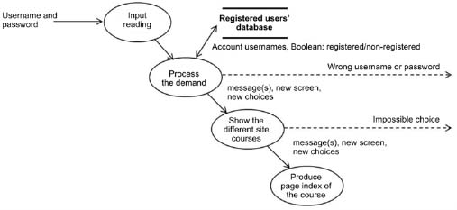
Figure 5.20. A data flow diagram integrating decision functions
More generally, in an object-oriented (OMT) approach, this set of data flow diagrams was built in order to clarify the meaning of operations and constraints, constituting what was agreed to be called the functional model. It is interested in data processing without regard to “sequencing, nor decisions, nor structure of the objects” [RUM 95, p. 178]. It shows how “output values in a calculation are derived from incoming values regardless of the order in which they are calculated” [RUM 95, p. 124].
We will see in Chapter 6 that the current object-oriented modeling languages like UML (which are actually just an extension of OMT) reflect this same intent with the so-called “use case” and “activities” diagrams. Use case diagrams provide an overview of a system’s functional behavior (corresponding to the OMT functional diagram); these activities allow a focus on processing. They are particularly suitable for modeling the data flow and allow us to graphically represent the behavior of an action or the progress of a use case.
We will mainly use these diagrams (derived from UML) in our modeling projects. We have provided arguments in section 5.2.5. They characterize a system “that does” clearly indicating the actions. Remember that the only reason leading us to previously introduce diagrams specific to OMT “techniques” or “methods” before those of UML stems from the fact that we recognized a founding language in OMT (possessing wanted assets), which developed current languages like UML in its different versions, UML 2 and SysML, etc.
5.3. Diachronic processes (the system becomes)
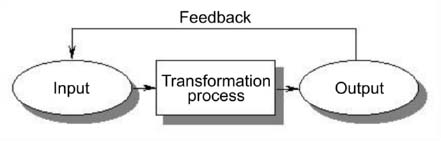
We have just represented the development of data registered at the heart of a finalized process circulating in an active environment. The data flow diagram shows functional dependencies between these values. At this third level of complexification, this helped highlight interrelationships among processes at a precise moment in time; in a static way: “the system performs”. But the canonical process model [RUM 95, p. 47] shows that it is also necessary to represent the system that transforms by “acting”, over time (see Figure 5.21).

Figure 5.21. The canonical process model [LEM 99, p. 47]
To arrive here, it is a matter of reaching the fourth level of archetype model complexification. In Rumbaugh et al.’s object and object-oriented modeling [RUM 95, p. 86], “these system aspects, dependent on time and changes, are grouped in the dynamic model...”. If we compare this model to the previous, we could say that if “the functional model indicates what is happening, the dynamic model indicates when this happens...” [RUM 95, p. 124]. We therefore propose that the modeler adopt this principle to explain, in a synchronic way, this “transforming” action in time. It is thus encouraged to describe the typical process phases (scenarios), highlighting the events that activate the actions. The traces left by these events will be useful in developing state diagrams that specifically account for expected “system state changes” at this level of complexification [LEM 99, p. 60].
Remember that at the fourth level of archetype model complexification:
“everything happens as if the system has endogenously produced intermediary forms, information, symbol systems, which would provide regulation intermediation [see RUM 95, p. 109] (thus the alleged electric impulse passing through nerves or a circuit transmits ‘regulation instructions’, ‘reflecting changes in the system state’). This symbolic emergence of information, artifact or internal communication device, constitutes an ‘event’ or jump, in the presumed complexification of the modeled system” [LEM 99, p. 60].
As we noted in the introduction to section 5.2, we approach this fourth level of complexification no longer in a static manner (the system “performs”) but according to its dynamic component (the system “becomes”). Notice again that the data flow diagrams previously proposed and constituting the DLE functional model respond to the first requirements at the fourth level of complexification. “The endogenous production of intermediary forms, information and symbol systems that provide regulation intermediation” seems well represented in these diagrams (information, pictograms, process input and output). The DLE dynamic model that we will now develop will be able to justify changes in the system state at this level of complexification.
We will begin by describing the typical process phases (scenarios), highlighting the events that activate the actions and transform them. We will then look at the traces left by these events. The latter will be useful for developing state diagrams at the end of section 5.3.3.
In object-oriented (OMT) modeling, diagrams represent the traces of action control which manifest through the translation of information exchanged and transformed during these activities.
5.3.1. Typical sequences (or scenarios) and even tracking
The word “scenario” has many meanings that adjust to the context in which it is used: cinema, management, education and informatics. Linking it to the context that we are concerned with (education/informatics), a scenario is described as a “set of events or behavior to describe the possible ‘evolutions’ of a system”26. This definition is not very far from the sense that books give on object-oriented modeling techniques: “a scenario is a sequence of event types; it allows for the description of common interactions for the extraction of events and the identification of target objects” 27 . The diagram is again the preferred instrument to represent the interface components and the system, as well as the courses that the users of the mechanism follow. “Each custom diagram becomes a bearer of cognitive activities that will place the user and the system in favorable contexts to interaction realization” [LEM 08, p. 132]. This leads us to specify actions performed on objects: this is the case, for example, when we click on an icon to specify an event type and the kind of cognitive activity that one maintains with the system. This can be the display of an illustration offered by way of explanation, that of a graphic text, or opening a window, allowing writing in order to communicate an opinion. The idea would be to make as many diagrams as there are events that will put the user in the presence of information or communication, either with the system or with others [LEM 08, p. 132]. Here, we will not give an example of diagram scenarios specific to object-oriented (OMT) modeling because we will have the opportunity to do so later when a specialized modeling language has been adopted (UML 2.0). We will then see that, in this language, the scenarios themselves are specific diagrams inside “use case” diagrams or “state transitions”. With that said, Lemire [LEM 08, pp. 132–136] proposes some examples of schematic scenario representations and a number of tips to build them. The reader can easily refer to his work if interested.
5.3.2. Traces left by events
The methodology implemented is based on the traces left by each of the activities, whether they are cognitive, informational, decision-making, organizational or regulatory. They are retrieved from surveys, semi-leading interviews with various actors of the considered DLE. We have collected much data on MOOCs upon their arrival in France in order to model these specific digital learning environments [TRE 15a, CHE 15a, CHE 15b]. This data tells us both about the perceptions and behavior of actors but also those of the registered users (students). This body of data can also result from specific computer applications introduced in DLEs in order to monitor training and its various actors (potential dropouts) online. These computer applications often provide accessible data in real time via a dashboard developed for this purpose. The BoardZ application that we will see later (Figures 5.28 and 5.29) is a good illustration of this. We will return in detail to this application in section 6.5.2 in Chapter 6 when dealing with data provenance and collection.
To collect these traces, we suggest combining two different approaches. The more pragmatic approach consists of collecting digital traces from learners with tracking tools. Often customizable, these tools allow for the modeling of the type of learning that you want to monitor. The goal is to be able to follow an area of study, be it from the teacher or student’s point of view, or even the institution’s. The data is often presented in the form of diagrams in educational monitoring “dashboards”28. The other approach is more traditional as it is based on surveys or semi-leading interviews.
5.3.3. The states and state diagrams
We resort to this to form the concept of state diagrams specific to Rumbaugh et al.’s “object-oriented modeling”29 language [RUM 95, p. 91]. These diagrams allow for the representation of action control traces which manifest through the translation of information exchanged and transformed during these activities30.

Figure 5.22. A state diagram constructed from an OpenClassrooms MOOC
In the same way that we stated for functional OMT diagrams in section 5.2, we can repeat this for OMT state diagrams above: the current object-oriented modeling languages in UML are able to translate this intention. In this precise case, they are concretely “state transition” diagrams that we have used in our “modeling projects” (see section 7.1.3 in Chapter 7 and Figure 6.12 in Chapter 6). We have given the arguments in section 4.2.5 in Chapter 4. They characterize an “evolving system” clearly indicating the different processor states.
5.3.4. Process descriptions
Remember that any complex system can be represented by a system of multiple actions or by a process that can be a tangle of processes, each of which can be represented by the designation of identified functions that it exercises or may exercise. The previous steps have allowed the designation of roles that these processes take, thus revealing values circulating in the mechanism to build and that are also exploited.
To portray them, the modeler focuses on what the system does and seeks to give an intelligible representation. This can be done in different ways: in natural language, pseudocode, mathematical formulation, using decision tables, etc. Rumbaugh [RUM 95, p. 181] recommends that the modeler “focus on what the function should do, not how to implement it. [...] The main goal is to show what happens in all cases”; thus, in the event of a free registration of an Internet user to an OpenClassrooms MOOC, the learning pace imposed (over 4 weeks).
5.4. A system capable of processing information and deciding its own behavior
A fifth level will now be added to the steps of systemic modeling complexification. The system becomes capable of deciding its own activity, processing the information that it produces and making decisions on its own behavior.
“Capable of generating information, the system becomes more complex by proving itself capable of handling: symbol computation, then cognitive exercise, the system becomes capable of developing its own behavioral decisions. It is necessary now to recognize an autonomous decision subsystem, processing information and only information in the model of the system” [RUM 95, p. 60].
The fifth level is a milestone in the progressive nature of the nine-level archetype model complexification process. The first four levels characterize cybernetic and structuralist procedures: the system has a project in an active environment; it exists, performs and transforms. The following levels first show the system’s ability to generate, process and store information (levels 5 and 6). Then, they identify it as capable of coordinating (level 7) and developing new projects and new action forms and being imaginative (level 8). Finall0079, the active process develops an auto-finalization ability which allows it to decide its own future and to make choices regarding its own direction (level 9).
5.5. A model based on analysis data
5.5.1. A model constructed from analysis data
The model’s construction is performed by successive iterations between the system of a constructed world and what the users perceive (their viewpoints) when they observe the realities or objects that constitute this world31.
“Possible discrepancies between the ‘system of the constructed world’ and the ‘system of the represented world’ should be identified at the time of audit from users of lesser or greater compliance (systems of the constructed and represented world). If adjustments are needed, they must be by successive iterations in order to minimize the distance between these two worlds as much as possible” [LEM 08, p. 108].
“Our vision of the world is a model. Any mental image is a model, fuzzy and incomplete, but serving as a base for decisions” [DER 75, p. 122].
From a first draft of solutions, systemic analysis proceeds by a permanent back and forth between a model to be built and the analysis data results provided by the system. “It is in this back and forth between data acquisition on the basis of modeling hypotheses and their reconstruction by modeling that a science of complex systems modeling can develop” [BOU 04b, p. 1]. The raw data collected is analyzed beforehand (data analysis) by applying such statistical procedures having recourse to multivariate techniques32 in view of system complexity and data variety. These techniques allow for the return of more synthetic and therefore simpler results by identifying and grouping the variables or terms that are similar (groups of “correlated” variables). These results constitute the analysis data which precisely allows for model refinement (examples to follow). The model is gradually constructed, taking into account this analysis data that reduces the distance between the systems of the constructed and represented world at each iteration.
“‘Modeling’ consists of building a model from the systems analysis data” [DER 75, p. 122].
5.5.2. Provenance and data collection
The data to analyze can be of all kinds: cognitive, informational, decision-making, organizational or regulatory. It can be surveys or interviews with different actors of a DLE or computer systems that can restore traces from a learner activity, like, for example, dashboards located on course platforms or tracking tools that allow for the identification of registered user profiles. It can also include simulation results that the modeler has decided to use in order to refine his model. All this data, produced and gathered by the modeler, allows for the determination of a succession of approximate solutions (analysis data) that are gradually approaching the perceived reality. It is therefore up to the modeler to determine what data is to be collected and retained, data that seems best adapted to the analysis context.
According to Cisel, for example,
“Early research on MOOCs is to a large extent based on learning trace analysis that can accurately measure what is happening on the teaching platform. But a purely descriptive approach of these usages is a problem if you want to understand the ins and outs of these behaviors on one side, and what is happening outside on the teaching platform on the other. To address these issues, more qualitative approaches derived from human and social sciences are essential: surveys, interviews, field observations; would it not be important to answer this simple question ‘Why subscribe to an MOOC?’” [CIS 16]
If the data provided by the system is plentiful and varied, the most relevant data to analyze is usually suggested to the modeler by the model itself. For example, the existence of a “forum” function registered at the heart of a model may encourage the modeler to want to know the reasons that motivate viewers to associate with it. He can question people affected by this mechanism in the form of interviews or questionnaires. These various kinds of data may possibly allow the modeler to discover that the forum function originally scheduled by the designer was transformed or converted, or simply that it has not been used... Conversely, the data analysis stemming from the system may reveal defects in the model’s internal structure which would correspond to the analysis data. This should alleviate the problem.
There are several non-exclusive data collection methods highlighted below and we will explain them in detail in the following sections. But if surveys, interviews and field observations are often preferred in the human and social sciences field, other means of collecting this data (tracking, simulation, etc.) can be useful to system analysis and to model improvement.
Among these analysis methods, the following are included:
- – analysis from data provided by tracking tools;
- – analysis from data provided by dashboards;
- – analysis from data provided by simulation;
- – analysis from data provided by questionnaires and interviews.
We will develop each of these methods in the following sections, and in Chapter 6 we will see concrete cases of modeling and analysis.
5.5.2.1. Data provided by tracking tools
Establishing activity traces involves highlighting the flow of information over communication activities, to show where the information is coming from and where it is going, the knowledge of the places where it is acquired, to specify how it is produced and operated, and to verify if the information flow is as planned and if communication is done according to expectations [LEM 08, p. 140].
There are several tracking tools which allow the participants’ actions in a DLE to be followed. The latter being specifically built on a web interface makes it easy, upon each visitor’s action, to send information using a tracker (a script33) to a statistical program that is installed on the web server and to store another part on the visitor’s computer via cookies (browsing history, identification information, etc.).
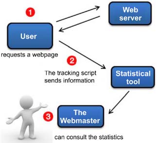
To perform this tracking, there are still several tools. The best known and most commonly used is Google Analytics. It writes the tracking code “in the websites’ source code in the location recommended by the statistical tool and on all pages of the site. If the website is made with a CMS, it will be necessary to insert this code in the page templates or functions called by the theme”34. The information is then processed by the statistical tool, and the webmaster can then view the results.
For example, here is what a tracking code in Google Analytics looks like:

With MOOCs being perfect representatives of the latest generation DLEs, they generate, just like other learning environments, traces of online activities that one can retrieve and process. In the second edition of MOOC EFAN (Enseigner et former avec le numérique), Boelaert and Khaneboubi [BOE 15] “counted more than 4,800 registered users and almost 500 activity deposits. The participants’ actions online generated traces of connections on MOOC servers (web logs) [...]. The logs are non-declarative information concerning those who log on to a website”. For them, it concerned “potentially interesting data in order to identify, for example, learner trajectories, typical behaviors or simply executing audience measurements” [BOE 15].
“[The recovered logs enabled them to] define five states for each user-week couple:
- –‘absent’: the user is never connected to the resources corresponding to this week;
- –‘present’: the user has connected to the pages of the week, but has not watched videos nor answered quizzes (he could download videos, or read, or simply visit pages to follow links to other sites);
- –‘video’: the user has watched at least one video of the week, but has not answered the quiz (unfortunately, the edX logs do not know if the user has uploaded a video, we know only if he looked at it directly on the course site);
- -‘view quiz’: the user has consulted the quiz of the week, but not answered it;
- -‘quiz’: the user has answered at least one question from the quiz of the week” [BOE 15].
Considering these representative states of degrees of investment in the MOOC, they draw “chronograms” for each week of courses and conclusions on these results. Figure 5.25 represents some of the participants who were in the five previous states, and Figure 5.26, constructed from the same data, represents the individual trajectories of all registered users in the form of a “carpet”35. The trajectories are arranged according to their end trajectory state [BOE 15].
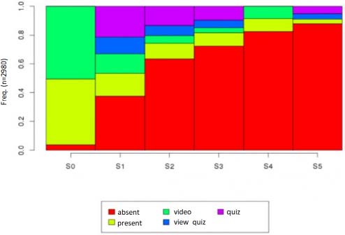
Figure 5.25. Frequency of the different states, week by week [BOE 15]. For a color version of this figure, see www.iste.co.uk/trestini/learning.zip
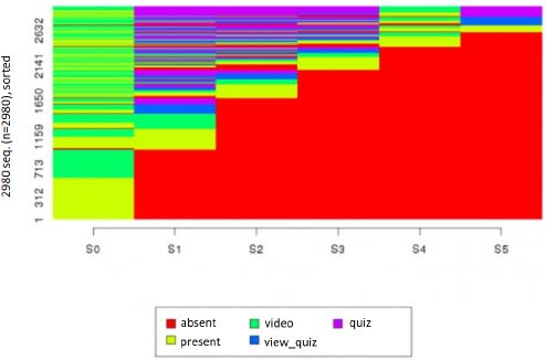
Figure 5.26. “Carpet” of the individual participants’ trajectories [BOE 15]. For a color version of this figure, see www.iste.co.uk/trestini/learning.zip
5.5.2.2. Data from reports generated by distance education platforms
Another simple and effective method is the analysis of connection data from reports generated by DLE platforms. Analysis of the traces left on the platform allows the teacher to learn more about his students’ activity via a PHP program. Figure 5.27 gives an example of analyses conducted from 2013 to 2015 by Éric Christoffel, a Professor and research colleague in our laboratory (LISEC), who wanted to know and precisely study his students’ activity in L3 MPC (Math-Physics-Chemistry). He also produced four graphs that allowed him to draw some interesting results:
- – video playback in minutes per day;
- – number of clicks on the course’s video page per day (correlated with the previous graph);
- – number of course notes consulted per day (PDF course notes);
- – number of downloads of various resources (in PDF format): subjects and correction, etc.
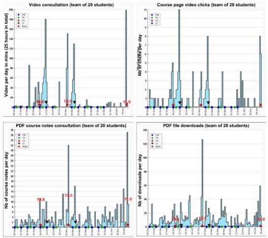
Figure 5.27. Data collected from reports generated by Moodle [THO 08]. For a color version of this figure, see www.iste.co.uk/trestini/learning.zip
In the first three graphs, it can be noted that the students are active the night before an examination or when a flipped classroom is imposed. In the last graph, it shows that students are regularly active throughout the year when it comes to downloading other resources: TD, TP text, subjects of previous years and corrected.
5.5.2.3. Data generated from dashboards: BoardZ project as an example
The Faculty of Avignon’s BoardZ project is an example of a generic tool located at the interface between the data collection mechanisms seen in the previous section and simulation. It is above all an educational dashboard engaged in distance learning. It is fully customizable with everyone possessing the ability to model the type of learning that he wants to oversee. One of the objectives of this project is to track the learning process of learners, in real time, in a distance learning environment. And it is from the teacher’s point of view, but also the student’s or the institution’s, offering an analysis of the digital footprints left by the learner. The project must therefore allow the teacher to make sure that everything goes “well” in his course, alert him as soon as possible in case of student dropout, give him a general trend of student practices, but also make an individual state by a student. In the same way, it gives the student the opportunity to position himself against the group’s practices and the teacher’s expectations. It must also allow the institution to “monitor” learning by presenting an overview of the practices in each lesson.
More specifically, particularly for FC, it is possible to model a generic response to accredited fund-collecting agencies concerning an intern’s course follow-up. The challenge is to be able to extract digital traces regarding learners’ activity to prove to accredited fund-collecting agencies that they have actually followed the course.
In summary, the educational dashboard project is a multitool allowing for:
- – the detection of early student dropouts;
- – the verification of consistency between the learners’ practices and the teacher’s expectations;
- – the facilitation of an individual learner monitoring in a course taught on-site or remotely;
- – the provision of evidence given by accredited fund-collecting agencies in lifelong education.
“BoardZ is an open source tool developed in Avignon that allows for the geographical viewing of educational indicators within a Moodle dashboard”. Several uses of this dashboard are possible depending on the user’s profile. Each profile has a progressive approach: from global to detailed. The global view allows for the comprehension of the whole area at a glance, while the following two levels offer a finer modeling of the objects of study selected. The viewing platform is generic and allows everyone to (re)define their own indicators by simply (re)writing SQL queries or redefining the functions to obtain the indicator values to customize.
The range that we present takes this data based on Moodle, but it can look for data in the school’s SI. For example, the teacher profile offers two previews for each of its courses on the first level, modeling ICT uses for one and the learners’ activity for the other. The second level presents the selected course activity of each learner in relation to others. Finally, the third level of precision displays indicators specific to one student for this course.
For each level, a warning system is available allowing the teacher, for example, from the first level of the teacher profile, to know that a learner has dropped one of his classes. In addition to the teacher profile there are: “student, training manager, platform administrator, ICT jury labelling profiles” [MAR 15]36.
According to Fanny Marcel and Thierry Spriet who are behind this project, this dashboard aims to promote student success by identifying dropouts as early as possible. They start from the realization that the Moodle platform reports are rather oriented toward individual monitoring, far from mass teaching. This dashboard must display an individualized profile by presenting relevant indicators while highlighting the abnormal behaviors. Pedagogical modeling combines several criteria (number of connections per week, access to resources (files, pages, etc.), activity on the forum, wiki, database, homework records, tests, etc., use of the type of graphic representations as seen in Figure 5.28).

Figure 5.28. A pedagogical BoardZ modeling combining five criteria
Access to different dashboards is possible: students/teachers/course managers. Each program actor is associated with a custom modeling. For example, the teacher will find a modeling type of each of its courses, activities, student dropout alerts, an overview of student activity and the ability to track each student individually. Figure 5.29 gives a brief overview of a French course list with a title, a description of the alerts and lists of students and models.
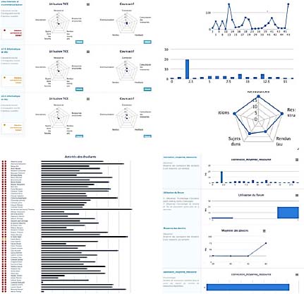
Figure 5.29. A project BoardZ pedagogical modeling. For a color version of this figure, see www.iste.co.uk/trestini/learning.zip
The goal today is to refine these pedagogical models, to integrate evaluations into their calculations and allow configuration of the course models (with the teachers’ expectations, etc.).
Work groups in which we have participated are currently hard at work to complete this project.
5.5.2.4. Simulation data
According to Rosnay [DER 75, p. 122], “simulation ‘tries to provide’ for a system allowing the simultaneous game of all variables; what limitations of our brain prohibit without computer assistance or simulation devices. Simulation is based on a model, itself established from prior analysis”.
“System analysis, modeling and simulation are thus the three fundamental steps in the study of the dynamic behavior of complex systems” [DER 75, p. 122].
Simulation is interesting when observing complex phenomena, because it allows for the simultaneous variation of variable groups, just as happens in reality. It is then possible to speculate hypotheses on observed phenomena, their behavior, to test initial conditions and to study the responses and reactions by varying them.
Simulation is therefore able to provide real-time responses to the various user decisions and actions; however, it requires powerful computers and, in some cases, cumbersome experimental editing. For example, to learn more about the influence of the wind on the lives of trees and plants, Emmanuel de Langre, Professor of mechanics at the École Polytechnique, and Pascal Hémon, a research engineer and aerodynamicist, installed a tree in a wind tunnel for the first time!37 From a DLE point of view, simulation does not require cumbersome mechanical means, but nevertheless, it requires the use of powerful computers capable of processing real-time variations of the multiple variables at play.
Simulating a complex system goes through a preliminary step of modeling system constituents, from their behaviors and interactions between these constituents and with their environment. The steps of this model structure have been described in detail at the beginning of Chapter 5. The next step consists of running the obtained model by mobilizing the appropriate computer means.
“One of the characteristics of these systems is that one cannot anticipate the evolution of the system modeled without going through this phase of simulation. The ‘experimental’ approach by simulation allows for the reproduction and observation of complex phenomena (biological or social, for example) in order to understand and anticipate their evolution”38.
Implementation is possible through behavioral simulations and multi-agents. Applicable to social sciences (social networks simulation), they allow for, in particular, the illustration of a number of perspectives from this domain and the interest of multidisciplinary approaches to address such systems.
There are many tools for the simulation of complex systems such as the multi-agent simulation platform (Netlogo, RePast, Gama, etc.), the dynamic systems platform (Stella) or even Anylogics, etc. As an example, Figure 5.30 illustrates an IRIT39 simulation in the multi-agent Netlogo simulation interface40.
5.5.2.5. Data provided by surveys, interviews and field observations
We have just seen that research based on the analysis of trace activities or simulation results allows for the former to precisely measure what is happening at the heart of the DLE subject to the study, and for the latter, to study its behavior in “real time”. But this purely descriptive approach can quickly be insufficient for those who want to understand the ins and outs of the phenomena observed. In fact, to address these issues in more detail, simultaneous quantitative and qualitative approaches, currently used in social sciences, become interesting insofar as they allow the researcher to be guided, offering him the ability to choose his own investigation targets (and not only those routinely provided by the platform). The tools at his disposal are traditional interviews, surveys and field observations.
In this regard, we speculate that the model that represents the DLE at any given moment helps the modeler to identify and choose relevant investigation targets and that conversely, the data analysis results, which will be gathered and processed following this investigation, will be used to improve the DLE model in construction (iterative process).

Figure 5.30. IRIT simulation on the multi-agent Netlogo simulation platform. For a color version of this figure, see www.iste.co.uk/trestini/learning.zip
The analysis that traditionally follows these surveys, interviews and field observations is generally of a confirmatory character. They are based in large part on inferential statistics that aim to test, according to a hypothetico-deductive approach, formulated hypotheses with the help of tests such as the chi-squared, Fisher or student’s t tests, to name but a few. They use the theory of probabilities to restrict the number of individuals by allowing surveys on samples. Hypothesis tests then allow for decision-making in situations involving a degree of chance. They are particularly useful when it comes to crossing several variables between them and to determining the level of significance of their functional dependencies. These so-called multivariate analyses function well when there are not too many variables to deal with and when you can easily make assumptions about their behavior in the system.
But as soon as one approaches the issue of highly complex systems, we are in the presence of so many variables and individuals (this not only in an MOOC) that these methods in turn show their limits. In addition, regarding phenomena that are often new and seldom documented (new generation DLE), hypotheses are difficult to formulate.
Actually, without completely prohibiting a few variable crossovers when it seems useful and opportune, we need to consider other analysis methods to deal with complexity, because as John Wilder Tukey jokingly said at the beginning of 1970s, an approximate answer to the right problem is worth a good deal more than an exact answer to an approximate problem41.
5.5.3. Data analysis
Once the data is collected, it is a matter of conducting the analysis itself. Facing complexity and interdependence, models are constructed based on the analysis we perform on data provided by the system, allowing the modeler to make assumptions on their overall behavior. This leads the modeler to experience “a model or design principles that can be used in the context of similar experiences” [HAR 09, p. 106].
We suggest using exploratory data analysis42 (EDA) since it relates to a complex system built up against descriptive statistics in order to deal with data retrieved from the different sources cited previously, namely:
- – dashboards, tracking tools;
- – simulation;
- – questionnaires and interviews.
At the beginning of model construction, data analysis collected cannot only be exploratory (Tukey [TUK 77] quoted by Cabassut [CAB 12]), but it should also eventually make hypotheses which may be validated or invalidated by a confirmatory analysis. This uses inferential statistics to test hypotheses in a deductive approach.
“[But] the practice rarely meets this scheme: you sometimes look to answer less specific questions, the data ‘pre-exists’ and has been collected according to complex surveys, there are absurd observations...” In these cases, their underlying hypotheses being violated, no longer have optimal classic methods. On the contrary, exploratory analysis starts from data and is based on observation logic. Thanks to a well-stocked toolbox, the explorer will look at his data from all sides, try to highlight structures, and, when appropriate, formulate plausible hypotheses” [LAD 97, p. 3].
But it would be absurd, as the author points out, to oppose classic statistics with exploratory statistics and equally absurd to want to confuse them.
“They both occupy a place of choice in statistical analysis and can prove to be complementary” [LAD 97, p. 4].
Thus, for us, exploratory data analysis developed particularly by Tukey [TUK 77], backed by descriptive statistics, appeared to be a good choice for processing data analysis from a complex system. We have since adopted it for our research, especially since “it can help in the construction of a model” [LAD 97, p. 4].
Exploratory data analysis (EDA) uses an inductive approach to describe the population (here the different actors who have, one way or another, participated in the DLE) and move around the formulation of hypotheses at the end of research. Exploratory analysis first aims to familiarize us with new phenomena, little or non-documented, and thus helps us make hypotheses for future research. The hypothesis is then at the end of research, and not at the beginning, as it is obligatory in a confirmatory analysis.
Furthermore, descriptive statistics that accompany and reinforce this exploratory analysis allows it to represent and synthesize numerous amounts of data provided by the system. “Descriptive statistics is the branch of statistics that brings together the many techniques used to ‘describe’ a relatively important grouping of data”43. And as pointed out by Cabassut and Villette [CAB 12], “it has the advantage of avoiding the constraints of sample representativeness”. Taking the example of teachers participating in a course, they remind us that they are not necessarily a representative sample of the teacher population.
“The institutional conditions vary greatly from one country to another; voluntary participant or participant designated by the school authority; training during working hours with a replacement professor or internship out of working time; an internship taken into account or not to advance career wise, etc” [CAB 12, p. 4].
For Joël Rosnay [DER 75, p. 122], continued by Tardieu et al. [TAR 86, p. 34], “system, modeling and simulation analysis constitute the three fundamental steps in the study of the dynamic behavior of complex systems” [TAR 86, p. 34].
During these past two years, we have engaged in a systemic modeling of the complexity approach in order to specifically study the behavior of several relatively popular MOOCs (project management, increasing MOOC from A to Z, EFAN and EFAN Math, etc.) seen as the latest generation DLEs. This work gave rise to four major publications:
- – a book on social MOOCs in France [TRE 16a], prefaced by Catherine Mongenet, a FUN project leader and resulting in the work of several researchers that we’ve directed within a seminar created for this purpose;
- – an article [TRE 15a] in the International Journal of Technologies in Higher Education, aiming to learn the perception of French actors in online teaching on this issue of MOOCs (which follows an announcement at the Montreal international conference (in Quebec);
- – an article [TRE 15b] published in The Online Journal of Distance Education and e-Learning, which presents our applied theoretical approach to “MOOCs in the paradigm of systemic modelling of complexity: some emerging properties”.
- – an article [TRE 17] presenting the modeling approach applied to help and support mechanisms offered in an MOOC. The publication is available on the journal website Distance et Médiatisation des saviors (DMS). This work has also opened the way for our future research program.