6
Modeling and Simulation of an MOOC: Practical Point
The modeling that we present below (which also partly serves to illustrate our approach) allows us to firstly provide a concrete illustration of what has been stated so far, and then to introduce our future research. In this chapter, we will therefore present this case before putting our mid-term research projects into perspective. Moreover, as this practical part serves as an example, it should be noted that we will follow the process of the systemic modeling of complexity developed in Chapter 5, by applying it to the specific case of a relatively well-known latest generation DLE: the Rémi Bachelet “Project management” MOOC (in its current version).
Through the model which has been gradually constructed, our goal was to first obtain a visual representation of this instrumented activity in order to sufficiently understand the behavior. Another objective, common to all visual models, was accessing a communication aid between the different actors involved in this project, whether they are mere users or researchers. Thus, it has been possible to more easily share what we have learned concerning this device with the educational and scientific community.
Among the different possible trajectories which leads us to systemic modeling (design, assessment, prospective analysis, etc.), we initially decided to limit ourselves to the analysis of system behavior in the hope of identifying some emerging properties (in a forward-looking approach). We have therefore supported, as recommended in section 6.5.2.4, a simulation program (in Python language) that we have written on the basis of this modeling1. Not having all the skills and energy necessary for the realization of this major project, we will only provide the founding elements of this program, emphasizing the rigor that is required, and before considering a more important development. In doing so, we want to show that our recommendations are not only theoretical but they quickly find concrete applications. In the near future, our intention is obviously to continue the development of this project by using more significant and more expert human and material resources.
6.1. Modeling an MOOC
Therefore, we wanted to model the “Project management” MOOC and attempt a simulation. Modeling an MOOC in its complexity involves first modeling a system of actions, in other words, identifying and formulating the functions performed by the system. We have done as described in section 6.1.1, bringing eight processors in a package diagram that we identified in section 6.1.4, corresponding to the eight constituent functions of any publicized educational environment. This diagram also represents the actors involved in each of the packages (Figure 6.1).
We then created our use case diagrams which represent, let us recall, children processors and functionalities specifically necessary for users. In UML, it is possible to make a use case diagram for a MOOC diagram in its entirety or for each package. Here, for reasons of readability, we have decided to produce a use case for each identified processor:
- – awareness (Figure 6.2);
- – production (Figure 6.3);
- – meta-reflexive activities (Figure 6.4);
- – management and planning (Figure 6.5);
- – social interactions (Figure 6.6);
- – assessment (Figure 6.7);
- – information (Figure 6.8);
- – support (Figure 6.9).

Figure 6.1. Package diagram based on the eight constituent functions of any publicized educational environment

Figure 6.2. “Awareness” use case diagram
In addition, remember that these diagrams are unique because they represent an organization which itself is unique: that of a “Project management” MOOC. It certainly presents similarities with other MOOCs, but it also develops specific features that require a personalized study. It is in this sense that we wanted to put ourselves closer to the formulations chosen by the MOOC, rather than apply ours. So, we will call “students” the people we would have rather named “enrolled” in another context, etc. However, we had no trouble gathering our various action complexes in the eight constituent functions of any publicized educational environment, made evident by the following package and “use case” diagrams
6.1.1. Package and use case diagrams
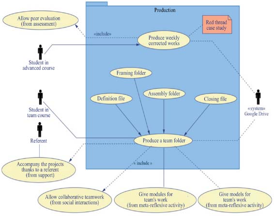
Figure 6.3. “Production” use case diagram
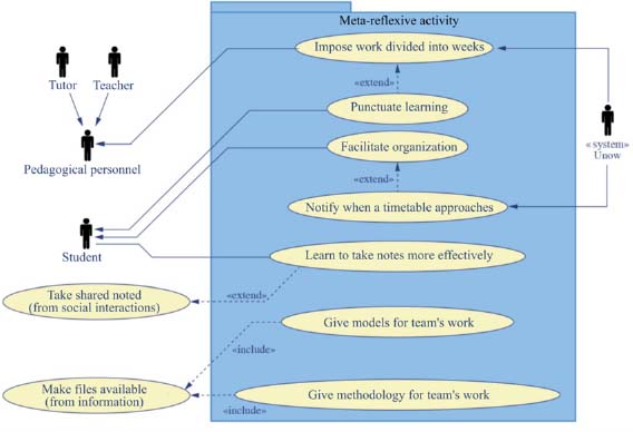
Figure 6.4. Meta-reflexive activities use case
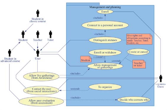
Figure 6.5. “Management and planning” use case

Figure 6.6. “Social interactions" use case diagram
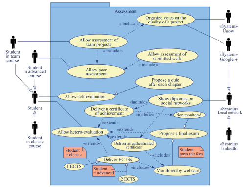
Figure 6.7. “Assessment” use case
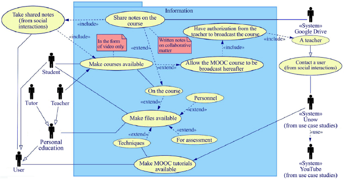
Figure 6.8. “Information” use case
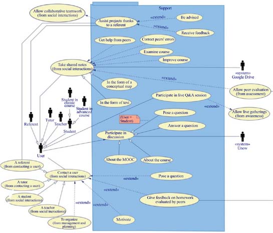
Figure 6.9. “Support” use case
6.1.2. “Class” diagrams
Once the system functions (or action complexes) are defined, we turned to the construction of class diagrams. Remember that this order is important in the systemic approach of complexity: it does not start by describing the system constituents, but its functions. Below, we give the project’s relatively representative class diagrams:
- – “Users” class (Figure 6.10);
- – “MOOC” class (Figure 6.11).
Remember that the usefulness of class diagrams, from the perspective of a simulation, is that they allow the definition of different “objects” involved in the activity: what are they, what attributes do they have and what are the relationships and actions between these objects?
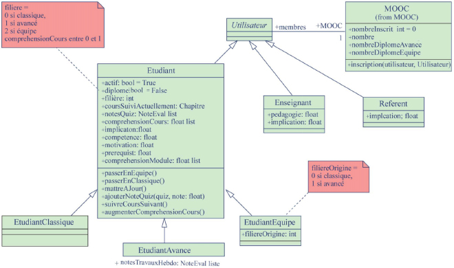
Figure 6.10. “Users” class diagram
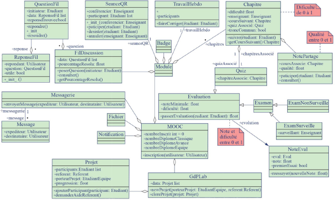
Figure 6.11. MOOC class diagram
We have a concrete example which shows that object-oriented modeling (OOM) and programming of the same name are perfectly suited to the study of complex systems. To show this, we note that the “constituent” concept of a system which is linked to other constituents (or itself) by “dependence relationships” finds a concrete representation in UML in the “object” concept connected by “operations”. Moreover, to code this system in terms of “classes” makes the code independent of initial conditions and fluctuations from the environment (noise), which are transcribed in the script2 (main.py, Figure 6.15). This independence is assured by a clear separation between the object-oriented architecture that lists the parameters and defines the possible interactions, and that collects and initializes the parameters, calling upon operations, interactions or methods. That is in part what makes this type of programming flexible.
Another flexibility factor lies in the fact that a class can be modified to affect all its instances.
Finally, by comparing languages in systemic modeling (SM) and object-oriented modeling (OOM), it is interesting to note that:
- – “the system that ‘is’” in SM is “embodied” in OOM “attributes”;
- – “the system that ‘performs’” in SM is found in the OOM “methods”3 that act on other objects (and can make them evolve);
- – “the system that ‘becomes’” in SM is found in specific or external methods (feedback) in OOM which, respectively, act or react to the studied object. The object becomes the target of methods that, when applied to it, make it evolve (methods that belong to the object or not).
OOM is very useful for modeling feedback. Calling a method in an object (initially, this is done in the script) generates a cascade of calls to various objects that can have a retroactive effect on the initial object for which the behavior will then be modified.
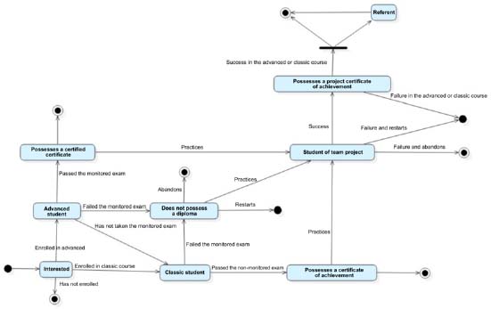
6.1.3. State transition diagrams
We have also resorted to UML state transition diagrams that reflect, as their name suggests, the different states of processors: they characterize an evolving system. State transition diagrams describe an object’s possible state changes in response to interactions with other objects or actors.
As an example, below, we give the state transition diagram of a student enrolled in a “Project management” MOOC.
6.1.4. Sequence diagrams
Sequence diagrams allow for the representation of collaborations between objects from a temporal point of view. These diagrams do not describe an object’s state, they focus on the expression of interactions. They can also be used to illustrate a use case. The order to send a message is determined by its position on the vertical axis of the diagram: time flows “from top to bottom” on this axis. The layout of objects on the horizontal axis has no effect on the diagram’s semantics.
State transition and sequence diagrams are the most important dynamic views in UML.
As an example, we give two sequence diagrams: “general course” (Figure 6.13) and discussion thread (Figure 6.14).
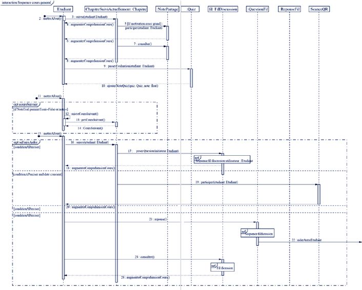
Figure 6.13. “General course” sequence diagram
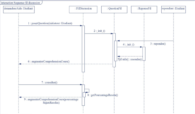
Figure 6.14. “Discussion thread” sequence diagram
6.2. MOOC simulation
Simulation is fundamentally based on the previous systemic model. It concretely formulates in an object-oriented programming language: here in the Python language. Other languages of this kind could do the trick. The export of UML object attributes and operations to the Python program structure was performed by an export feature specific to the modeling software (Tools => Python => Generate code). Now, let us look at the program structure and the script that must be distinguished.
6.2.1. The program structure
The program structure reflects the structure of the MOOC studied. Thus, the “Project management” MOOC is fundamentally composed of
- – a set of modules which themselves consist of a set of chapters;
- – a set of users “specializing”4 in students, teachers, tutors and referents.
A student may specialize in “classic” or “advanced” and, if he has enough experience, in “student project by team”. A student is also defined by a number of attributes that will characterize his “learning” and “level of understanding” of the chapter, module or MOOC in progress. A student can “update”5 (consisting of performing a series of operations including “read the course” and “answer the quiz”) and skip to the next chapter (with all modifications ensuing on his level of understanding).
A chapter is composed of attributes (difficulty, associated teacher and associated quiz) and a method (view the course). If this method is called, it will also have a retroactive effect on the student (passed as a parameter) viewing the course and increasing his level of understanding of it, according to a law dependent on all parameters.
A quiz is also an attribute (its difficulty) and a method (answering the quiz). This method also has an influence on the student (passed as a parameter): this shall be assigned a note that characterizes the student even further.

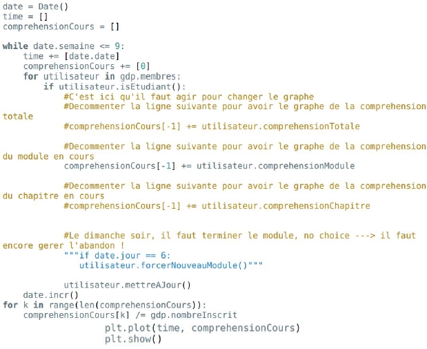
Figure 6.15. Main.py script
6.2.2. The script
The script takes place in three significant times as well as the temporal dimension of the simulation (Figure 6.15):
- – MOOC initialization (initialization du MOOC): learn about the “MOOC” object by assigning modules, chapters and a teacher;
- – registration phase (phase d’inscription): assign students to the MOOC (here, for example, 900 in a classic course and 100 in an advanced course);
- – learning phase (phase d’apprentissage): for every day of the course, for every student, “update” this (makes it read the course, answers the quiz, etc.). It is the “eleve.mettreAJour()” method that is responsible for this operation.
6.2.3. Related files
Many other files are clearly associated with this script but are not immediately essential to the understanding of the program. We have decided to only provide a few as examples (see Appendices 3–5) to avoid unnecessarily overloading the book.
6.2.4. Parameters that come into play and initialization values
In this example of simulation, the parameters that characterize the main objects are:
- – for the student: his commitment, competence, motivation, prerequisites, uniformly chosen at random between 0 and 1;
- – for the course: its difficulty, set at 0.5 by default;
- – for the teacher (there is only one): his pedagogy, his involvement, set to 1 by default.
Note that if all stated parameters were at 1, the simulation predicts that the student would understand everything perfectly the first time.
We have therefore assigned the student a random score following a normal distribution centered on his level of understanding with a standard deviation of 0.1. For example, if his level of understanding is 0.6, he will probably get 0.6 as a quiz score but will also be able to get a score of 0.5 or 0.7.
6.2.5. Progress in the chapters
A student always tries the quiz twice to get the best possible score, unless he has obtained a score of 1 on the first attempt. If he has earned a score of 1 on the first quiz or has taken the quiz twice, he will proceed to the next chapter. Otherwise, he passes the quiz with a probability of 0.6.
6.3. Simulation result
Would it be surprising to get the simulation results that correspond to nothing we expected to observe? Not really if one refers to the theories of SM developed thus far. According to the latter, we should rather expect to observe the unexpected phenomena and even counter-intuitive effects. And it is the latter that we have witnessed. Indeed, wanting to study variations in the level of understanding of the course by students according to random initial conditions, we expected to obtain different levels of understanding. And against all odds, we have instead seen an amazing regularity in the system response (homeostasis).
But let us make no mistake, and it is not so much this result that interests us in the first place, it is rather the implementation approach to achieve this result. That said, let us go over in detail regarding what an MOOC systemic modeling is and what its simulation allowed us to discover.
One of the observable phenomena of the very simplified model presented here as an example is a representation of the students’ level of understanding. There are three levels:
- – the level of understanding of the chapter (niveauComprehensionChapitre), which corresponds to the understanding of the chapter of the course being studied;
- – the level of understanding of the module (niveauComprehensionChapitre), which corresponds to the understanding of the chapter of the course being studied;
- – the level of total understanding (niveauComprehensionTotale), which is the understanding of the entire MOOC.
It should be noted that the level of understanding of the module is the average of the levels of understanding of all the chapters of the module and that the level of total understanding of the course is the average of all levels of understanding of all proposed chapters in the MOOC.
In the sections that follow, we provide the average of all students of the three aforementioned variables based on time.
6.3.1. Level of total understanding
The curve below is the average of all the MOOC’s levels of total understanding from all students according to the time (in days).
We observe a growing understanding that slows toward the end of the MOOC. This slowdown is explained by the fact that the fastest students have already finished the MOOC and stop progressing.
6.3.2. Level of understanding of the module
The curve shown in Figure 6.17 corresponds to the average of all the MOOC’s levels of understanding of the module from all students according to the time (in days).

Figure 6.16. The average of all levels of understanding of MOOC total of all students/day

Figure 6.17. The average of all levels of understanding of the module from all the students/day
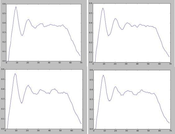
Figure 6.18. The average of all levels of understanding of the module from all the students/day/random experience
The shape of this curve leads us to make four comments:
- – first observation: oscillations. This is explained by the fact that a student sees his level of understanding of the module evolving “unevenly”: he increases his understanding during the module, and when he moves to the next module, he begins with a void level of understanding. This is quite normal as he starts to appropriate new knowledge. But there is also an oscillation of the value of this quantity when considering the average of all students;
- – second observation: damped oscillations. The curve clearly shows damped oscillations (we can even venture to see an amplitude which decreases in exponential decreasing, etc.). This is explained by a progressive phase shift of students. At the beginning of the MOOC, all students start at the same time, which translates into a very fast growth, and then they are faced with a new module all at the same time, which translates into a very fast decline. But as students learn at different rates, some find themselves at the end of a module and therefore have a high level of understanding, while others have already begun a new module and have a low level of understanding. In physics, this is called a dispersion phenomenon: the wave packet diminishes because the phase speeds of the different superimposed harmonic waves are different;
- – third observation: at the end of the MOOC, the level of understanding falls. We explain this phenomenon for technical reasons. When a student has finished the MOOC curriculum, he is no longer associated with a module, and therefore his level of understanding of the module remains void. This decline means that different students do not complete the MOOC simultaneously;
- – fourth observation: we observe a certain regularity in the system response subject to variations in the initial conditions.
In response to the completely random parameters supplied to the system, we can notice local fluctuations on the graph (especially in the damped part) when the initial conditions change (for different experiences), but the overall curve shape (damped oscillations) remains substantially the same.
6.3.3. Level of understanding of the chapter
We observe a similar phenomenon to the level of understanding of the chapter.
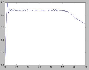
Figure 6.19. The average of all levels of understanding of the chapter from all the students/day
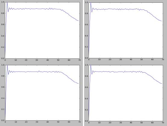
Figure 6.20. The average of all levels of understanding of the chapter from all the students/day/random experience
At this point, it would be bold to immediately conclude the existence of any emergent phenomenon, revealing the stability of the system (its homeostatic nature) as long as it is subject to very different initial conditions. It was necessary for us to spend more time studying this regularity and try other tests, and this is not the desired goal here. Nevertheless, this result suggests the possibility of identifying, or even demonstrating, the recurrence of a behavior during different events (changes in the initial conditions) and allows for the revealing of the general causes and mechanisms to finally describe the different forms.
6.4. Putting the obtained results into perspective
One might say that the study of a “comprehensionChapitre” variable has no great benefit because it does not reflect the actual level of a registered user. However, we can imagine that one registered user understands the course he is reading (therefore starting the course) very little and will tend to ask questions on a forum while a registered user understanding the course more fully (finishing the course) would be more independent. This could translate into forums that are oscillating in attendance and, additionally, damped. It would have to be verified in the facts; but if that were proven, this result would be useful to possibly predict the sufficient number of tutors present on the forum to answer questions from registered users.
Such a model, clearly expanded and adapted, can observe the unexpected phenomena, which can confirm or deny the field’s validity. But such models are superior to the simple observation, because they allow access to all the states of all participants at any moment, making the observation of any size possible.
It is also important to remember that the result obtained was not very foreseeable, and we do not necessarily intuitively think that we should study the attendance of the forums over time...
These are clearly just examples that may seem trivial compared to the modeling work that this requires. But nevertheless, they lead us to believe that this program (constructed according to the recommended modeling approach) was not used a lot (for lack of time and resources), while it already offers, such as it is, an interesting potential for the behavior analysis of Rémi Bachelet’s MOOC. It goes without saying that our goals are now to develop this model and its simulation program to produce further understanding about MOOCs and more generally the latest generation DLEs. Today, there are indeed a number of simulation techniques that allow for the observation of a complex system behavior to very varying degrees of abstraction and detail.