
Learning how to learn is life’s most important skill.
—Tony Buzan, Writer and Educational Consultant
As the content we find we need to learn changes throughout life, we find new methods of learning that work for us. Through your education, you might have considered brute-force solving dozens of repetitive, minimally varying problems to be helpful when mastering the basics of algebra, active reading with a highlighter and notes on hand to help you succeed in more advanced English classes, and, later on with more advanced topics, understanding the conceptual framework and intuition more helpful than rotely solving a series of problems.
Ultimately, the task of learning is not just one of optimizing your mastery of the content within certain learning conditions but of optimizing those very learning conditions. To become efficient agents and designers of learning processes, we must recognize that learning is multi-tiered, controlled not only by our progress within the learning framework an agent may currently be operating in but also the learning framework itself.
This necessity applies to neural network design. Designing neural networks involves making many choices, and many of these can often feel arbitrary and therefore unoptimized or optimizable. While intuition is certainly a valuable guide in building model architectures, there are many aspects of neural network design that a human designer simply cannot effectively tune by hand, especially when multiple variables are involved.
Meta-optimization, also referred to in this context as meta-learning or auto-ML, is the process of “learning how to learn” – a meta-model (or “controller model”) finds the best parameters for the controlled model’s validation performance. With its tools and knowledge about its underlying dynamics and best use cases, meta-optimization is a valuable box of methods to aid you in developing more structured, efficient models.
Introduction to Meta-optimization
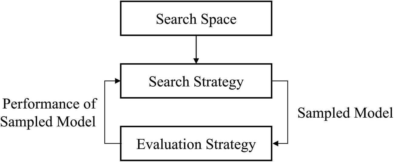
A deep learning model is already a learner itself, optimizing its designated weights to maximize its performance on the training data it is given. Meta-optimization involves another model on a higher level optimizing the “fixed” parameters in the first model such that the first model, when trained under the conditions of those fixed parameters, will learn weights that maximize its performance on the test dataset (Figure 5-1). In machine learning – a domain in which meta-optimization is frequently applied – these fixed parameters could be factors like the gamma parameter in support vector classifiers, the value of k in the k-nearest neighbors algorithm, or the number of trees in a gradient boosting model. In the context of deep learning – the focus of this book and thus the application of meta-optimization in this chapter – these include factors like the architecture of the model and elements of its training procedure, like the choice of optimizer or the learning rate.
Here, we use the terms “parameters” and “weights” selectively for the sake of clarity, even though the two are more or less synonymous. “Parameter” will refer to broader factors in the model’s fundamental structure that remain unchanged during training and influence the outcome of the learned knowledge. “Weight” refers to changeable, trainable values that are used in representing a model’s learned knowledge.
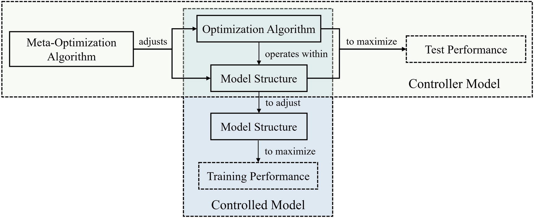
Relationship between controller model and controlled model in meta-optimization
- 1.
Select structural parameters for a proposed controlled model.
- 2.
Obtain the performance of a controlled model trained under those selected structural parameters.
- 3.
Repeat.
Grid search: In a grid search, every combination of a user-specified list of values for each parameter is tried and evaluated. Consider a hypothetical model with two structural parameters we would like to optimize, A and B. The user may specify the search space for A to be [1, 2, 3] and the search space for B to be [0.5, 1.2]. Here, “search space” indicates the values for each parameter that will be tested. A grid search would train six models for every combination of these parameters – A = 1 and B = 0.5, A = 1 and B = 1.2, A = 2 and B = 0.5, and so on.
Random search: In a random search, the user provides information about a feasible distribution of potential values that each structural parameter could take on. For instance, the search space for A may be a normal distribution with mean 2 and standard deviation 1, and the search space for B might be a uniform choice from the list of values [0.5, 1.2]. A random search would then randomly sample parameter values and return the best performing set of values.
Grid search and random search are considered to be naïve search algorithms because they do not incorporate the results from their previously selected structural parameters into how they select the next set of structural parameters; they simply repeatedly “query” structural parameters blindly and return the best performing set. While grid and random search have their place in certain meta-optimization problems – grid search suffices for small meta-optimization problems, and random search proves to be a surprisingly strong strategy for models that are relatively cheaper to train – they cannot produce consistently strong results for more complex models, like neural networks. The problem is not that these naïve methods inherently cannot produce good sets of parameters, but that they take too long to do so.
A key component of the unique character of meta-optimization that distinguishes it from other fields of optimization problems is the impact of the evaluation step in amplifying any inefficiencies in the meta-optimization system. Generally, to quantify how good certain selected structural parameters are, a model is fully trained under those structural parameters and its performance on the test set is used as the evaluation. (See the “Neural Architecture Search” section for proxy evaluation to learn about faster alternatives). In the context of neural networks, this evaluation step can take hours. Thus, an effective meta-optimization system should attempt to require as few models to be built and trained as possible before arriving at a good solution. (Compare this to standard neural network optimization, in which the model queries the loss function and updates its weights accordingly anywhere from hundreds of thousands to millions of times in the span of hours.)
- 1.
Select structural parameters for a proposed controlled model.
- 2.
Obtain the performance of a controlled model trained under those selected structural parameters.
- 3.
Incorporate knowledge about the relationship between selected structural parameters and the performance of a model trained under such parameters into the next selection.
- 4.
Repeat.
Even with these adaptations, meta-optimization methods are taxing on computational and time resources. A primary factor in the success of a meta-optimization campaign is how you define the search space – the feasible distribution of values the meta-optimization algorithm can draw from. Choosing the search space is another trade-off. Clearly, if you specify too large a search space, the meta-optimization algorithm will need to select and evaluate more structural parameters to arrive at a good solution. Each additional parameter enlarges the existing search space by a significant factor, so leaving too many parameters to be optimized by the meta-optimization algorithm will likely perform worse than user-specified values or a random search, which doesn’t need to deal with the complexities of navigating an incredibly sparse space.
Herein lies an important principle in meta-optimization design: be conservative in determining parameters to be optimized by meta-optimization as possible. If you know that batch normalization will benefit a network’s performance, for instance, it’s probably not worth it to use meta-optimization to determine if batch normalization should be included in the network architecture or not. Moreover, if you decide a certain parameter should be optimized via meta-optimization, attempt to decrease its “size.” For instance, this could be the number or range of possible values a parameter can take on, the range of possible values.
On the other hand, if you define too small a search space, you should ask yourself another question – is meta-optimization worth performing in the first place? A meta-optimization algorithm is likely to find the optimal set of parameters for a search space defined as {A: normal distribution with mean 1 and standard deviation 0.001 and B: uniform distribution from 3.2 to 3.3} very efficiently, for instance, but it’s not useful. The user could have likely set A=1 and B=3.25 with no visible impact on the resulting model’s performance.
What is a “small” or “large” range is dependent on the nature of the parameter and the variation required to make visible change in the performance of the model. Parameters sampled from a normal distribution with mean 0.005 and standard deviation 0.001 may yield a very similar model if that parameter is the C parameter in a support vector machine. However, if the parameter is the learning rate of a deep learning model, it is likely that such a distribution would yield visible differences in model test performance.
Thus, the crucial balance in meta-optimization is that of engineering a search space conservative enough not to be redundant, but free and “open” enough to yield significant results.
This chapter will discuss two forms of meta-optimization as applicable to deep learning: general hyperparameter optimization and Neural Architecture Search (NAS), along with the Hyperopt, Hyperas, and Auto-Keras libraries.
General Hyperparameter Optimization
General hyperparameter optimization is a broad field within meta-optimization concerning general methods to optimize the parameters of a wide variety of models. These methods are not explicitly built for neural network designs, so additional work will be required for effective results.
In this section, we’ll discuss Bayesian optimization – the leading general hyperparameter optimization method for machine and deep learning, as well as the usage of the popular meta-optimization library Hyperopt and its accompanying Keras wrapper, Hyperas, to optimize neural network design.
Bayesian Optimization Intuition and Theory
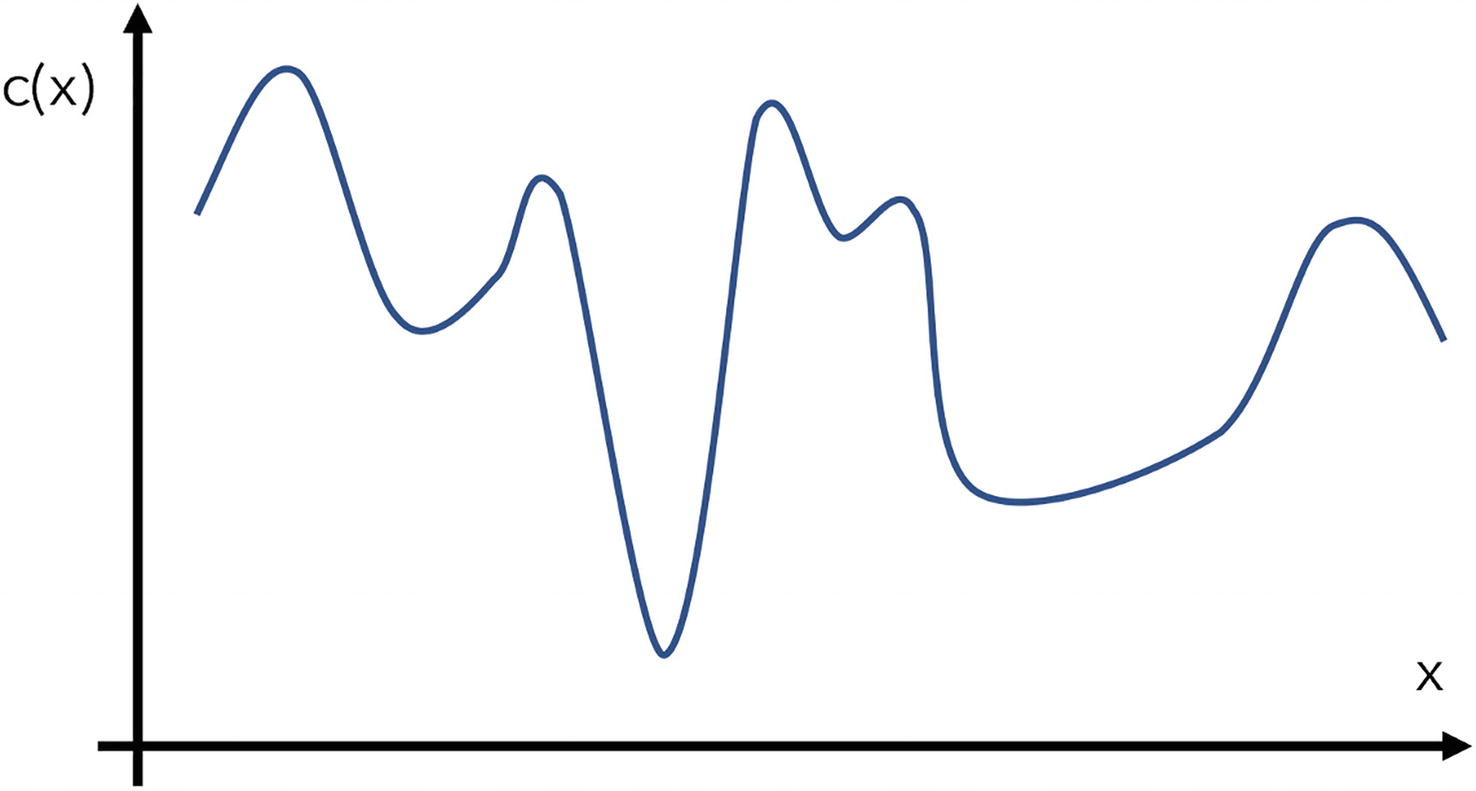
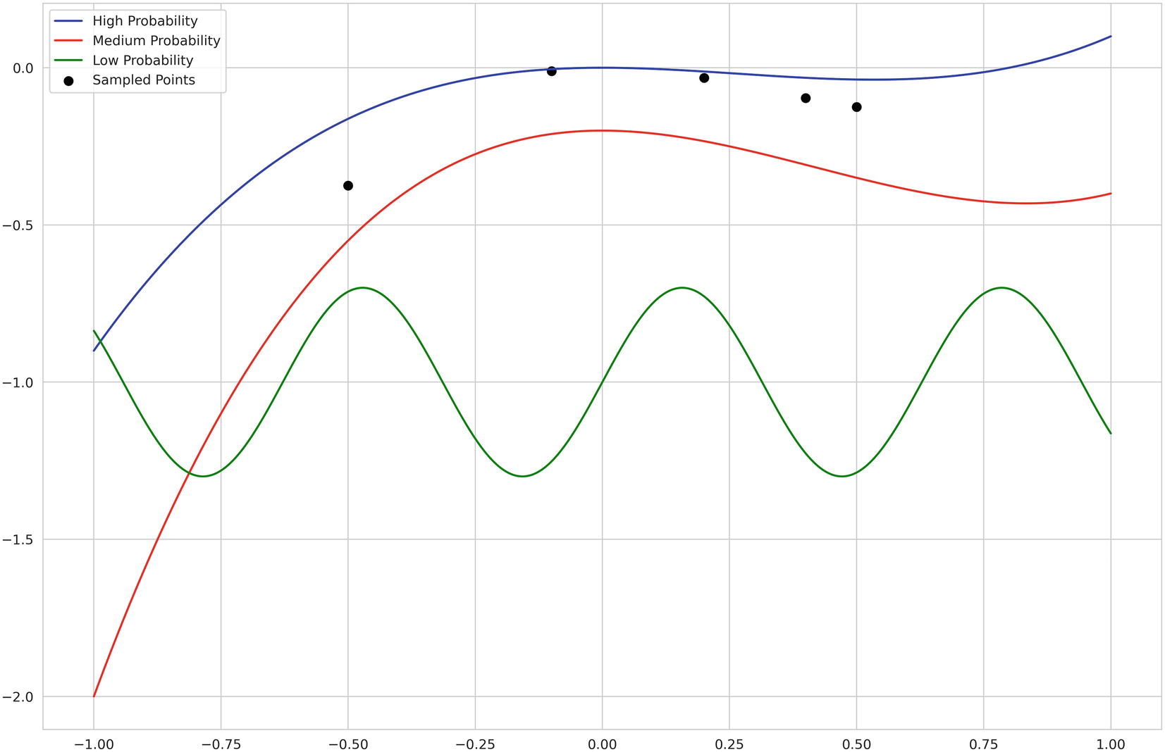
Here’s a function: f(x). You only have access to its output given a certain input, and you know that it is expensive to calculate. Your task is to find the set of inputs that minimizes the output of the function as much as possible.

Objective functions to minimize. Top – black-box function; bottom – explicitly defined loss function (in this case MSE)
Bayesian optimization is often used in these sorts of black-box optimization problems because it succeeds in obtaining reliably good results with a relatively small number of required queries to the objective function f(x). Hyperopt, in addition to many other libraries, uses optimization algorithms built upon the fundamental model of Bayesian optimization. The spirit of Bayesian modeling is to begin with a set of prior beliefs and continually update that set of beliefs with new information to form posterior beliefs. It is this spirit of continuous update – searching for new information in places where it is needed – that makes Bayesian optimization a robust and versatile tool in black-box optimization problems.
Hypothetical cost function – the loss incurred by a model with some parameter x. For the sake of visualization, in this case we are optimizing only one parameter
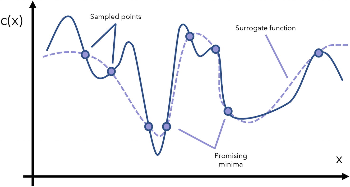
Example surrogate function and how the surrogate function informs the sampling of new points in the objective function
Note that the representation of the surrogate model here is deterministic, but in practice it is a probabilistic model that returns p(y| x) or the probability that the objective function’s output is y given an input x. Probabilistic surrogate models are easier and more natural to update in a Bayesian function.
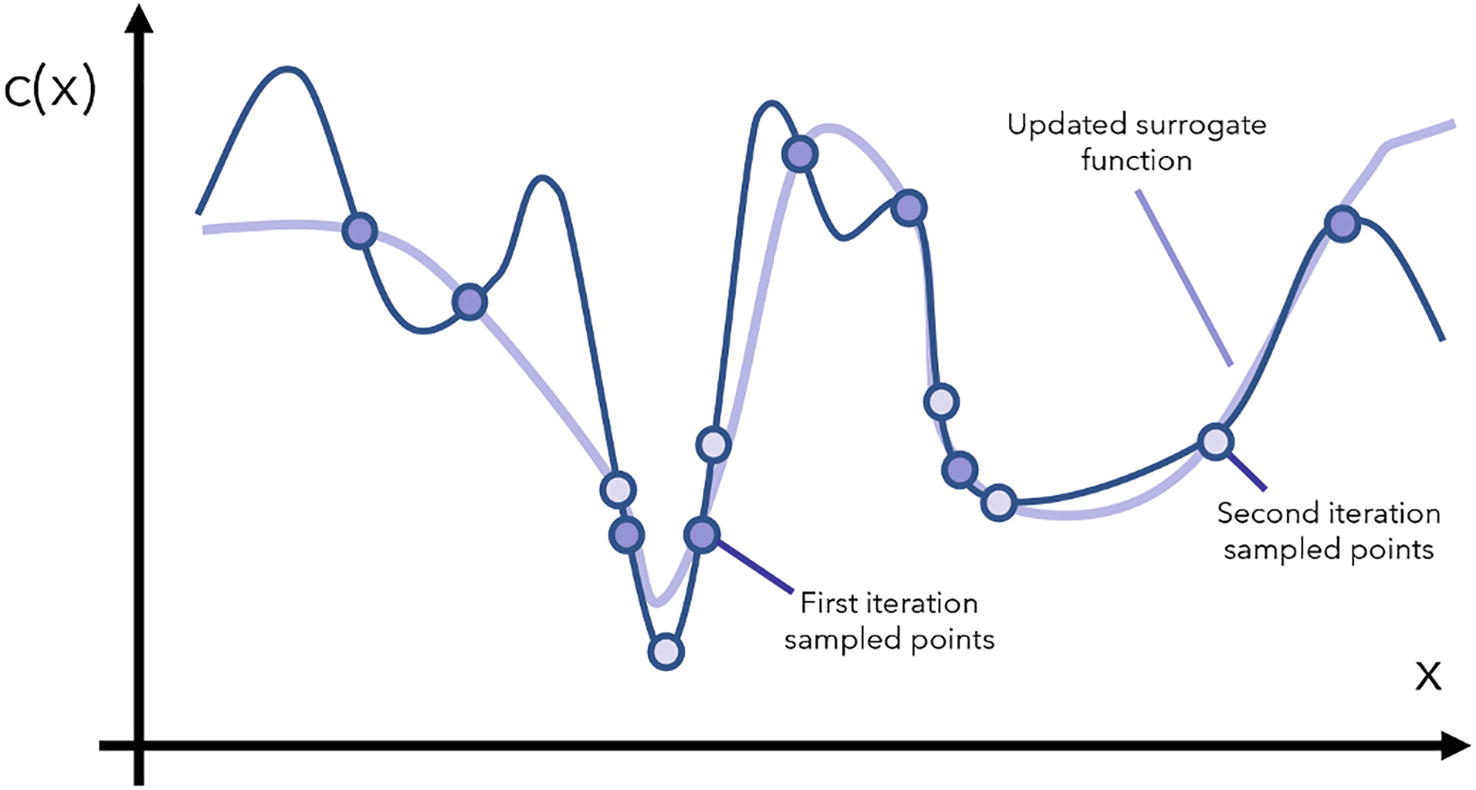
Updating the surrogate function with the new, second iteration of sampled points
After just a few number of iterations, there is a very high probability that the Bayesian optimization algorithm has obtained a relatively accurate representation of the minima within the black-box function.
Because a random or grid search does not take any of the previous results into consideration when determining the next sampled set of parameters, these “naïve” algorithms save time in calculating the next set of parameters to sample. However, the additional computation Bayesian optimization algorithms use to determine the next point to sample is used to construct a surrogate function more intelligently with fewer queries. Net-wise, the reduction in necessary queries to the objective function outweighs the increase in time to determine the next sampled point, making the Bayesian optimization method more efficient.
This process of optimization is known more abstractly as Sequential Model-Based Optimization (SMBO) . It operates as a central concept or template against which various model optimization strategies can be formulated and compared and contains one key feature: a surrogate function for the objective function that is updated with new information and used to determine new points to sample. Across various SMBO methods, the primary differentiators are the design of the acquisition function and the method of constructing the surrogate model. Hyperopt uses the Tree-structured Parzen Estimator (TPE) surrogate model and acquisition strategy.
The expected improvement measurement quantifies the expected improvement with respect to the set of parameters to be optimized, x. For instance, if the surrogate model p(y| x) evaluates to zero for all values of y less than some threshold value y∗ – that is, there is zero probability that the set of input parameters x could yield an output of the objective function less than y∗ – there is likely little improvement.

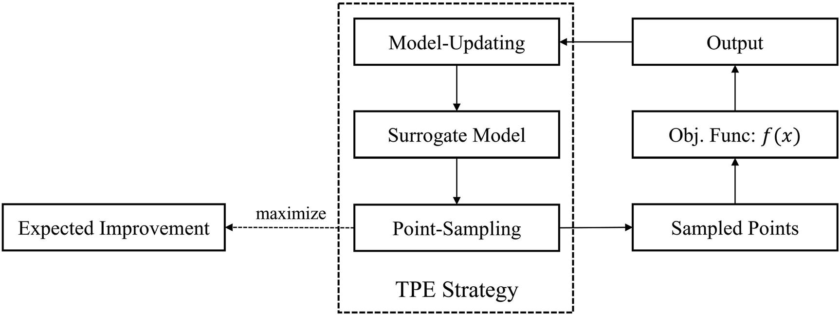
Visualizing where the Tree-structured Parzen Estimator strategy falls in relation to the Sequential Model-Based Optimization procedure
It’s a little bit math heavy, but ultimately the Tree-structured Parzen Estimator strategy attempts to find the best objective function inputs to sample by continually updating its two internal probability distributions to maximize the quality of prediction.
You may be wondering – what is tree-structured about the Tree-structured Parzen Estimator strategy? In the original TPE paper, the authors suggest that the “tree” component of the algorithm’s name is derived from the tree-like nature of the hyperparameter space: the value chosen for one hyperparameter determines the set of possible values for other parameters. For instance, if we are optimizing the architecture of a neural network, we first determine the number of layers before determining the number of nodes in the third layer.
Hyperopt Syntax, Concepts, and Usage
Objective function : This is a function that takes in a dictionary of hyperparameters (the inputs to the objective function) and outputs the “goodness” of those hyperparameters (the output of the objective function). In this context of meta-learning, the objective function takes in the hyperparameters, uses the hyperparameters to build a model, trains the model, and returns the performance of the model on validation/test data. “Better” is synonymous with “less” in Hyperopt, so make sure that metrics like accuracy are negated.
Search space : This is the space of parameters with which Hyperopt will search. It is implemented as a dictionary of parameters in which the key is the name of the parameter (for your own reference later) and the corresponding value is a Hyperopt search space objective defining the range and type of distribution to sample values for that parameter from.
Search : Once you have defined the objective function and the search space, you can initiate the actual search function, which will return the best set of parameters from the search.
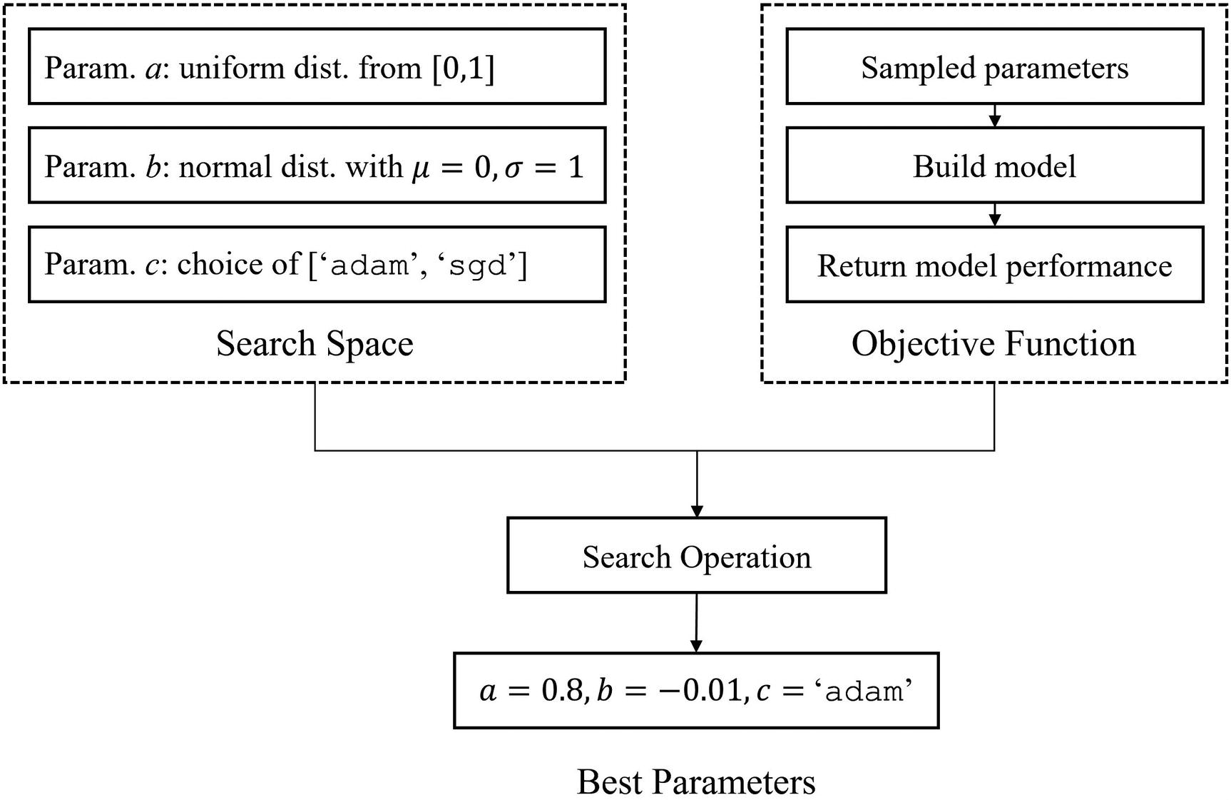
Relationship between the search space, objective function, and search operation in the Hyperopt framework
Install Hyperopt with pip install hyperopt and import with import hyperopt.
Hyperopt Syntax Overview: Finding the Minimum of a Simple Objective Function
Importing the Hyperopt library and defining the search space for a single parameter using hyperopt.hp
hp.normal(label, mu, sigma): The distribution of the search space for this parameter is a normal distribution with mean mu and standard deviation sigma.
hp.lognormal(label, mu, sigma): The distribution of the search space for this parameter is a log-normal distribution with mean mu and standard deviation sigma. It acts as a modification of hp.normal that returns only positive values. This is useful for parameters like the learning rate of a neural network that are continuous and contain a concentration of likelihood at some point, but require a positive value.
hp.qnormal(label, mu, sigma, q) and hp.qlognormal(label, mu, sigma, q): These act as distributions for quasi-continuous parameters, like the number of layers or number of nodes within a layer in a neural network – while these are not continuous (a network with 3.5 layers is invalid), they contain transitive relative relationships (a network with 4 layers is longer than a network with 3 layers). Correspondingly, we may want to formulate certain relationships, like wanting the number of layers to be shorter than longer. hp.qnormal and hp.qlognormal “quantize” the outputs of hp.normal and hp.lognormal by performing the following operation:
 , where o is the output of the “unquantized” operation and q is the quantization factor. hp.qnormal('x', 5, 3, 1), for instance, defines a search space of “normally distributed” integers (q = 1) with mean 5 and standard deviation 3.
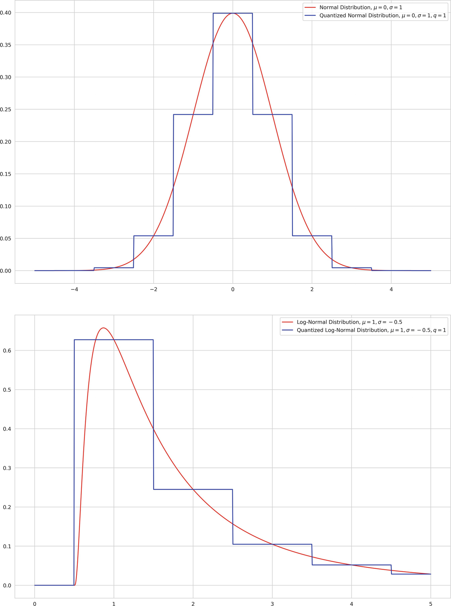
Visualizations of the normal and quantized normal distributions (top) and the log-normal and quantized log-normal distributions (bottom). The quantized distribution visualization is not completely faithful – values that fall into a sampled “segment” are assigned the same value
If the search space is not continuous or quasi-continuous, but instead a series of discrete, non-comparable choices, use hp.choice(), which takes in a list of possible choices.
Defining a simple Hyperopt space
We can now define the objective function, which simply involves subtracting 1 from x and squaring: obj_func = lambda params: (params['x']-1)**2.
Only returning the associated output of the objective function is fine if the objective function always returns a valid output or you have configured the search space such that it is impossible for any invalid input to be passed into the objective function. If not, however, Hyperopt provides one additional feature that may be helpful if certain combinations of parameters may be invalid: a status. For instance, if we are trying to find the minimum of  , the input x = 0 would be invalid. There’s no easy way to restrict the search space to exclude x = 0, though. If x ≠ 0, the output of the objective function is {'loss':value, 'status':'ok'}. If the input parameter is equal to 0, though, the objective function returns {'status':'fail'}.
An objective function with ok/fail status
Hyperopt minimization procedure
Here, algo=tpe.suggest uses the Tree-structured Parzen Estimator optimization algorithm and max_evals=500 lets Hyperopt know that the code will tolerate a maximum 500 evaluations of the objective function. In the context of modeling, max_evals indicates the maximum number of models that will be built and trained, because each evaluation of the objective function requires building a new model architecture, training it, evaluating it, and returning its performance.
After the search completes, best is a dictionary of the best parameters found. best['x'] should contain a value very close to 1 (the true minimum).
Using Hyperopt to Optimize Training Procedure
hp.choice('optimizer', ['adam', 'rmsprop', 'sgd']) for the optimizer: This will find the optimal optimizer to train the network on.
hp.lognormal('lr', mu=0.005, sigma=0.001) for the optimizer learning rate: The log-normal distribution is used here because the learning rate must be positive.
Defining a search space for model optimizer and learning rate
- 1.
Build the model: We will use a simple sequential model with a convolutional and fully connected component. This can be built without accessing the params dictionary because we’re not tuning any hyperparameters that influence how the architecture is built.
- 2.
Compile: This is the relevant component of the construction and training of the model because parameters we are tuning (optimizer and learning rate) are explicitly used in this step. We will instantiate the sampled optimizer with the sampled learning rate and then pass the optimizer object with that learning rate into model.compile(). We will also pass metrics=['accuracy'] into compiling such that we can access the accuracy of the model on the test data in evaluation as the output of the objective function.
- 3.
Fit model: We fit the model as usual for some number of epochs.
- 4.
Evaluate accuracy: We can call model.evaluate() to return a list of loss and metrics calculated on the test data. The first element is the loss, and the second is the accuracy; we index the output of evaluation accordingly to assess the accuracy.
- 5.
Return negated accuracy on validation set: The accuracy is negated such that smaller is “better.”
Defining the objective function of a training procedure-optimizing operation
Note that we specify verbose=0 with both model.fit() and model.evaluate(), which prevents Keras from printing progress bars and metrics during training. While these progress bars are helpful when training a Keras model in isolation, in the context of hyperparameter optimization with Hyperopt, they interfere with Hyperopt’s own progress bar printing.
We can use the objective function and the search space, along with the Tree-structured Parzen Estimator and the maximum number of evaluations, into the fmin function: best = fmin(objective, space, algo=tpe.suggest, max_evals=30).
After the search has completed, best should contain a dictionary of best performing values for each parameter specified in the search space. In order to use these best parameters in your model, you can rebuild the model as it is built in the objective function and replace the params dictionary with the best dictionary.
Early stopping callback: This stops training after performance plateaus to save as many resources (computational and time-wise) as possible, as meta-optimization is an inherently expensive operation. This can usually be coupled with a high number of epochs, such that each model design is trained toward fruition – its potential is extracted as much as reasonably possible, and training stops after there seems to be no more potential to extract.
Model checkpoint callback with weight reloading before evaluation: Rather than evaluating the state of the neural network after it has completed training, it is optimal to evaluate the best “version” of that neural network. This can be done via the model checkpoint callback, which saves the weights of the best performing model. Before evaluating the performance of the model, reload these weights.
These two measures will further increase the efficiency of the search.
Using Hyperopt to Optimize Model Architecture
Although Hyperopt is often used to tune parameters in the model’s training procedure, you can also use it to make fine-tuned optimizations to the model architecture. It’s important, though, to consider whether you should use a general meta-optimization method like Hyperopt or a more specialized architecture optimization method like Neural Architecture Search. If you want to optimize large changes in the model architecture, it’s best to use Neural Architecture Search via Auto-Keras (this is covered later in the chapter). On the other hand, if you want to optimize small changes, Auto-Keras may not offer you the level of precision you desire, and thus Hyperopt may be the better solution. Note that if the change in architecture you intend to optimize is very small (like finding the optimal number of neurons in a layer), it may not be fruitful to even optimize it at all, provided that you have set a reasonable default parameter.
Number of layers in a certain block/component (provided the range is long enough): The number of layers is quite a significant factor in the model architecture, especially if it is compounded via a block/cell-based design.
Presence of batch normalization: Batch normalization is an important layer that aids in smoothing the loss space. However, it succeeds only if used in certain locations and with a certain frequency.
Presence and rate of dropout layer: Like batch normalization, dropout can be an incredibly powerful regularization method. Successful usage of dropout requires placement in certain locations, with a certain frequency, and a well-tuned dropout rate.
For this example, we’ll tune three general factors of the model architecture: the number of layers in the convolutional component, the number of layers in the dense component, and the dropout rate of a dropout layer inserted in between every layer. (You could also tune the dropout rate of all dropout layers, which offers less customizability but may be more successful in some circumstances.)
Because we are keeping track of the dropout rate of several dropout layers, we cannot merely define it as a single parameter in the search space. Rather, we will need to automate the storage and organization of several parameters in the search space corresponding to each dropout layer.
Defining key parameters
Creating an organized list of dropout rates
Note that we are constructing as many search space variables as the maximum number of layers for the convolutional and fully connected components, which means that there will be redundancy if the number of layers sampled is less than the maximum number (i.e., some dropout rates will not be used). This is fine; Hyperopt will handle it and adapt to these relationships. Additionally, we are defining a normal search space for the dropout rate that could theoretically sample values less than 0 or larger than 1 (i.e., invalid dropout rates). We will adjust these within the objective function to demonstrate custom manipulation of the search space when Hyperopt does not provide a function that fits your particular needs (in this case, a normal-shaped distribution that is bounded on both ends).
Defining the search space for optimizing neural network architecture
Building the objective function in this context is an elaborate process, so we’ll build it in multiple pieces.
Recall that the Hyperopt search space for the dropout rate was defined to be normally distributed, meaning that it is possible to sample invalid dropout rates (less than 0 or larger than 1). We can address sampled parameters that are invalid at the beginning of the objective function (Listing 5-10).
Beginning to define the objective function – correcting for dropout rates sampled in an invalid domain
Defining the model template and input in the objective function
Building the convolutional component in the objective function
Building the dense component in the objective function
Afterward, append the model output and perform the previously discussed remaining steps of compiling, fitting, evaluating, and returning the output of the objective function.
As you can see, Hyperopt allows for a tremendous amount of control over specific elements of the model, even if it involves a little bit more work – your imagination (and your capability for organization) is the limit!
Hyperas Syntax, Concepts, and Usage
Hyperopt offers a tremendous amount of customizability and adaptability toward your particular optimization needs, but it can be a lot of work, especially for relatively simpler tasks. Hyperas is a wrapper that operates on Hyperopt but is specialized in syntax for meta-optimizing Keras models. The primary advantage of Hyperas is that you can define parameters to be optimized with much fewer code than Hyperopt syntax requires.
While Hyperas is a useful resource, it’s important to know how to use Hyperopt because (a) often, problems that require meta-optimization in the first place are complex enough to warrant using Hyperopt and (b) Hyperas is a less developed and stable package (it is currently archived by the owner). Additionally, be warned that there are complications with using Hyperas with Jupyter Notebooks in an environment like Kaggle or Colab – if you are working with these circumstances, it may be easier to use Hyperopt.
Install Hyperas with pip install hyperas and import with import hyperas.
Using Hyperas to Optimize Training Procedure
Data feeder function : A function must be defined to load data, perform any preprocessing, and return four sets of data: x train, y train, x test, and y test (in that order). By defining the data feeding process as a function, Hyperas can make shortcuts to prevent redundancy in data loading in training the model.
Objective function : This function takes in the four sets of data from the data feeder function. It builds the model with unique markers for parameters to be optimized, fits on the training data, and returns whatever loss is used for evaluation. The objective function should return a dictionary with three key-value pairs: the loss, the status, and the model the loss was evaluated on.
Minimization : This function takes in the objective function (model creating function) and the data feeder function, alongside the Tree-structured Parzen Estimators algorithm from Hyperopt and a max_evals parameter. Because Hyperas is implemented with lots of recording, the minimization procedure requires a hyperopt.Trials() object, which serves as an additional documentation/recording object. (You can also pass this into fmin() for Hyperopt, although it’s not required.)
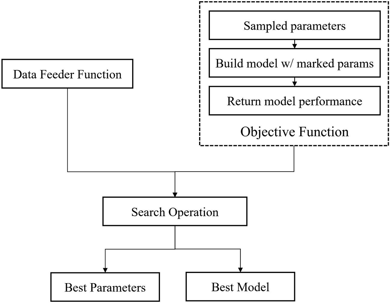
Key components of the Hyperas framework – data feeder, objective function, and search operation
Assuming the data feeder function has already been created, we will create the objective function (Listing 5-14). It is almost identical to the objective function in Hyperopt, with two key differences: the objective function takes in the four sets of data rather than the parameters dictionary, and optimizable parameters are defined completely within the objective function and with as little user attachment and handling as necessary.
Objective function for optimizing training procedure in Hyperas
Optimizing in Hyperas
After training, you can save the model and parameters for later usage.
Using Hyperas to Optimize Model Architecture
Objective function for optimizing architecture in Hyperas
This objective function can then be used in hyperas.optim.minimize() as usual.
The same dropout rate is used in every added layer by defining only one dropout rate that is repeatedly used in each dropout layer
Neural Architecture Search
In our previous discussion of meta-optimization methods, we have used generalized frameworks for the optimization of parameters in all sorts of contexts that are also applicable to neural network architecture and training procedure optimization. While Bayesian optimization suffices for some relatively detailed or non-architectural parameter optimizations, in other cases we desire a meta-optimization method that is designed particularly for the task of optimizing the architecture of a neural network.
Neural Architecture Search (NAS) is the process of automating the engineering of neural network architectures. Because NAS methods are designed specifically for the task of searching architectures, they are generally more efficient in finding high-performing architectures than more generalized optimization methods like Bayesian optimization. Moreover, because Neural Architecture Search often requires searching for practical, efficient architectures, many view NAS as a form of model compression – building an architecture that can effectively represent the same knowledge as a larger architecture more effectively.
NAS Intuition and Theory
Many of the well-known deep learning architectures – ResNet and Inception, for instance – are built with incredibly complex structures that require a team of deep learning engineers to conceive and experiment with. The process of building such structures, too, has never quite been a precise science, but instead a continual process of following hunches/intuition and experimentation. Deep learning is such a quickly evolving field that theoretical explanations for the success of a method almost always follow empirical evidence rather than vice versa.
Neural Architecture Search is a growing subfield of deep learning, attempting to develop structured and efficient searches for the most optimal neural network architectures. Although earlier work in Neural Architecture Search (early 2010s and before) used primarily Bayesian-based methods, modern NAS work involves the usage of deep learning structures to optimize deep learning architectures. That is, a neural network system is trained to “design” the best neural network architectures.
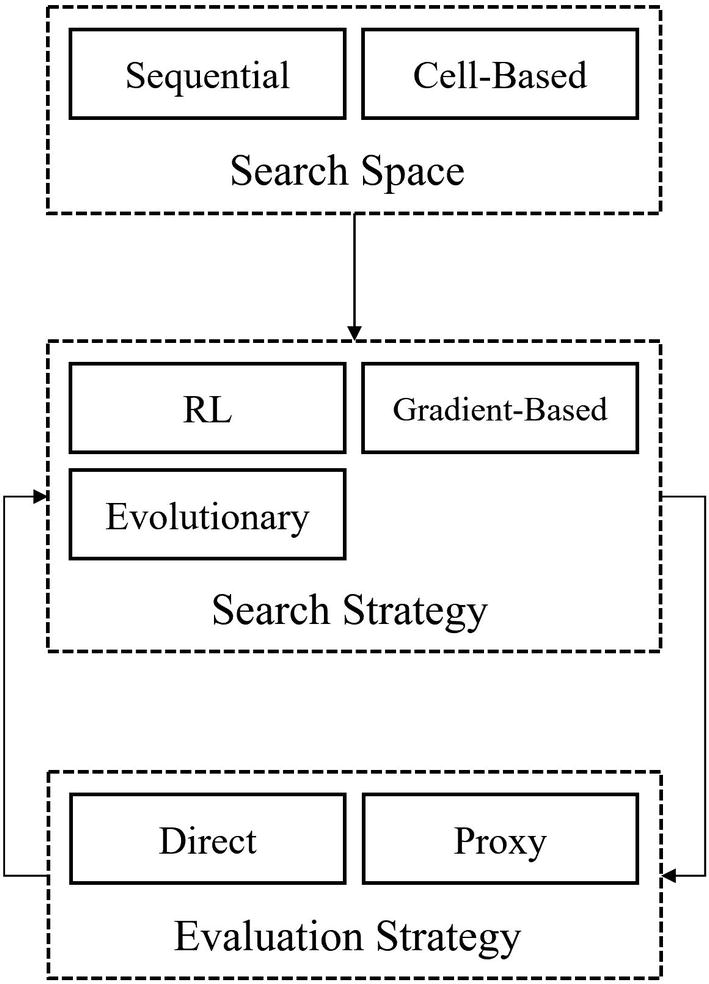
Relationship between three key components of Neural Architecture Search – the search space, the search strategy, and evaluation strategy
This is a similar structure to how Bayesian optimization frameworks perform optimization. However, NAS systems are differentiated from general optimization frameworks in that they do not approach neural network architecture optimization as a black-box problem. Neural Architecture Search methods take advantage of domain knowledge about neural network architecture representation and optimization by building it into the design of all three components.
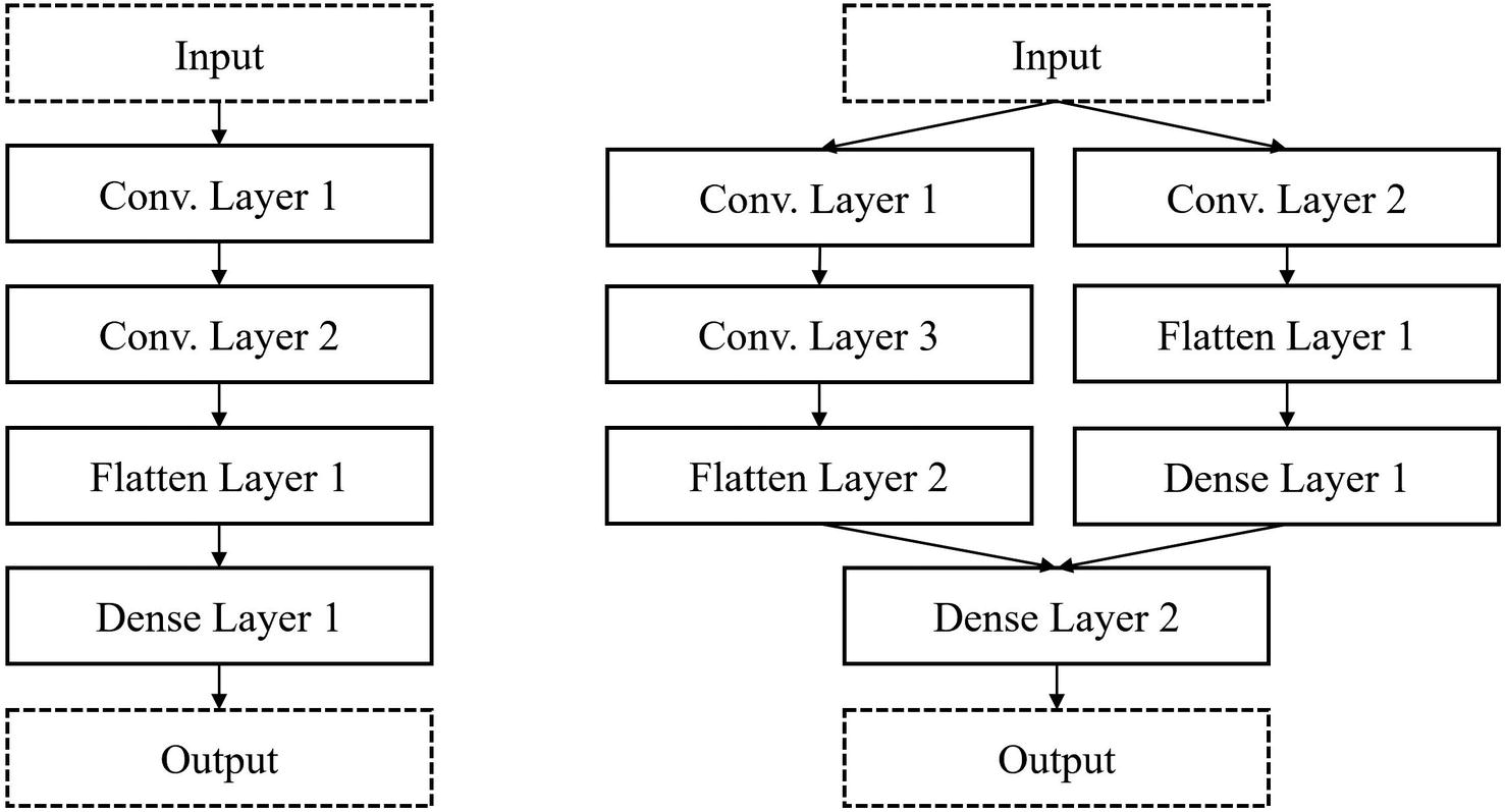
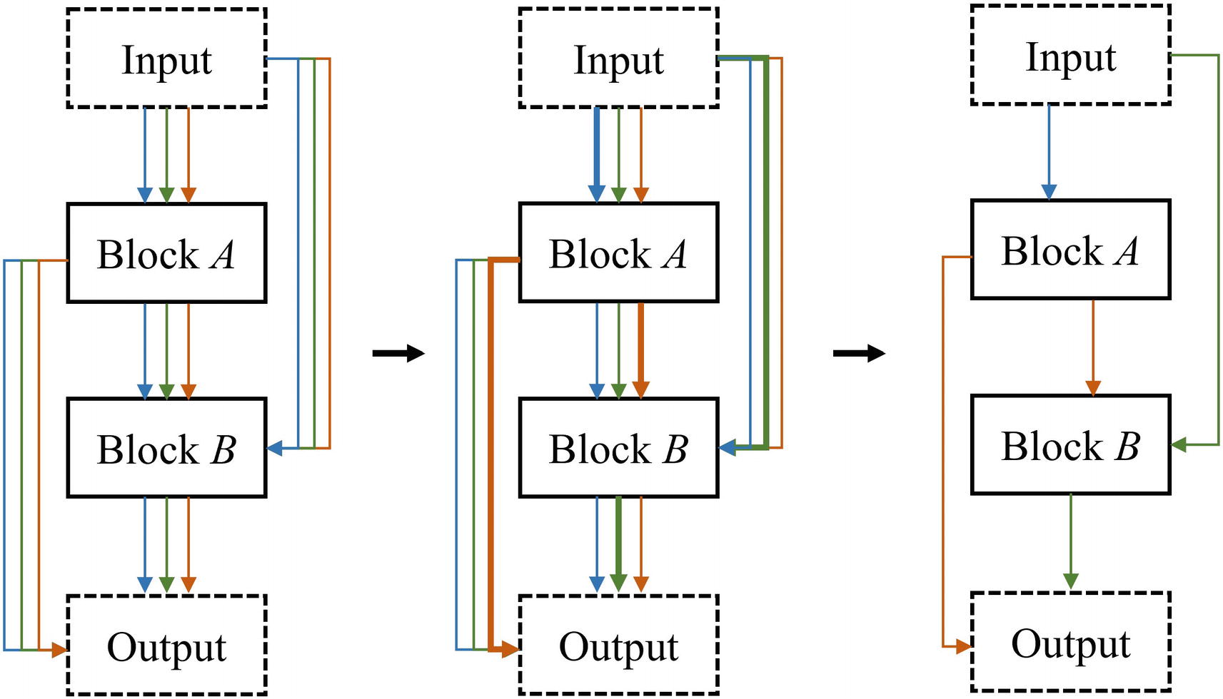
Left – a sequential topology; right – a more complex nonlinear topology
Moreover, the search space must be capable of representing both linear and nonlinear neural network topologies, which further complicates the organization of such a search space.
Note that Neural Architecture Search systems go to tremendous trouble to represent neural networks in seemingly contrived ways primarily for the purposes of the search strategy component , not the search space itself. If the only purpose of the search space component is to represent the model, current graph network implementations more than suffice. However, it’s incredibly difficult to create a search strategy that is able to effectively output and work with a neural network architecture in that exact format. The medium of the search space representation allows the search strategy to output a representation, which can be used to build and evaluate the corresponding model. Moreover, limiting the search space to only certain architecture designs likely to be successful forces the search strategy to sample from and explore more high-potential architectures.
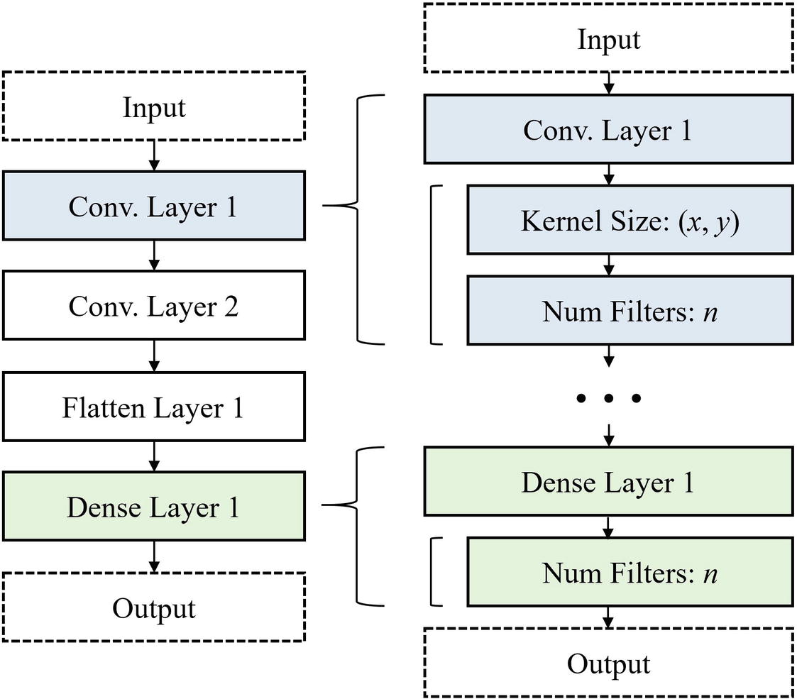
Sequential representation of a linear neural network topology
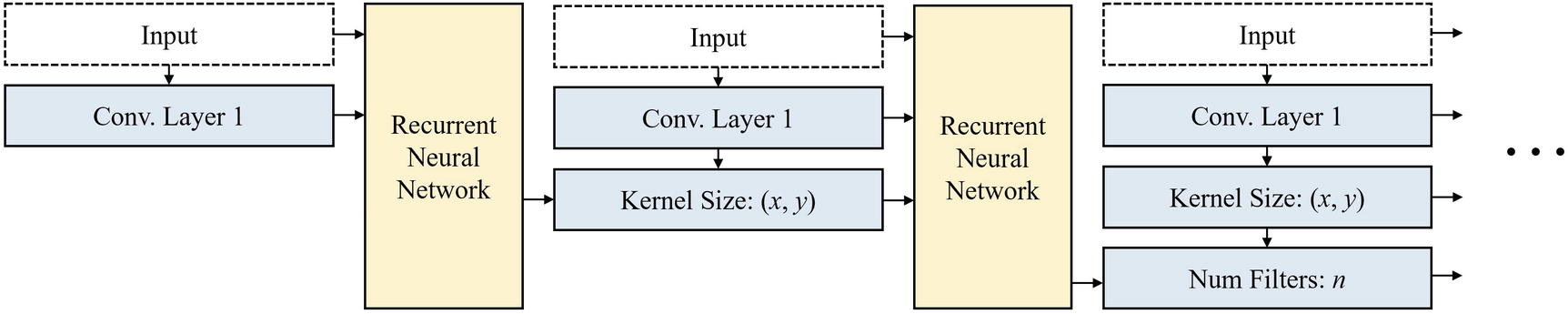
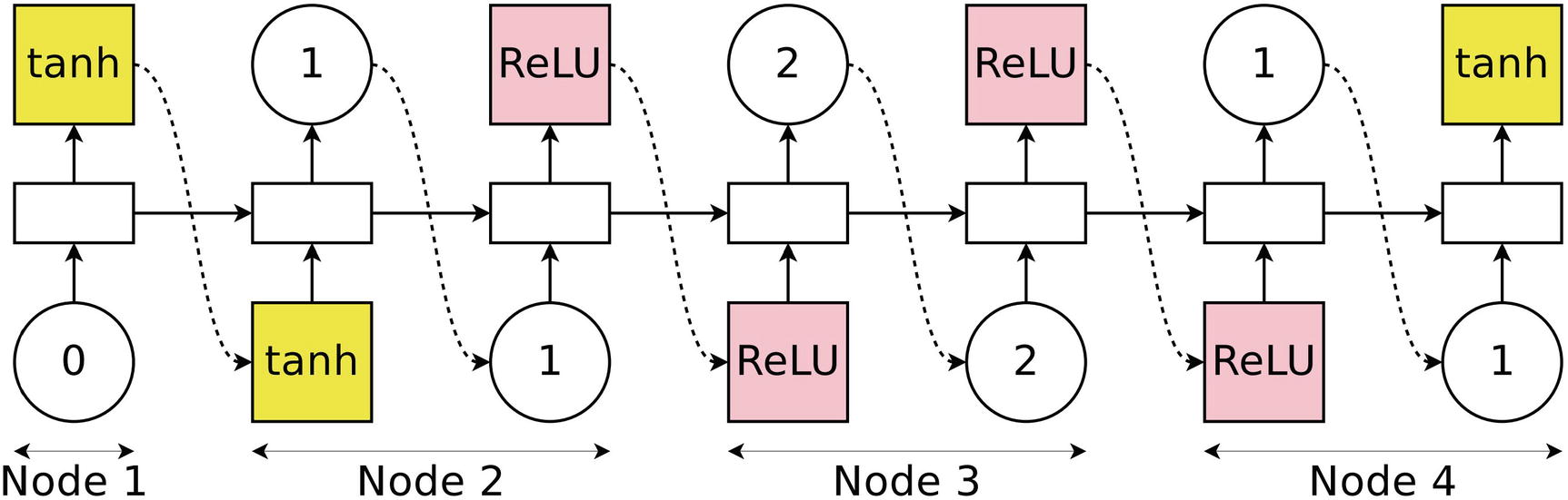
Additional adaptations can be made to represent more complex nonlinear topologies and recurrent neural networks by incorporating indices and “anchor points” into the sequential string of information. Skip connections can be modeled via an attention-style mechanism, in which the modeling agent can add skip connections between any two anchor points. The sequential string representation is powerful in that any neural network architecture – regardless of how complex – can be represented in and rebuilt from this format, even if it takes a very long sequence of information.
This sort of sequential representation was used to represent the search spaces of earlier NAS work by Barret Zoph and Quoc V. Le in 2017. The sequential representation of the search space, while being powerful (i.e., it can model many neural network architectures), proved not to be very efficient. Because the search space is so large, however, sequential representations of neural networks proved to be inefficient to navigate.
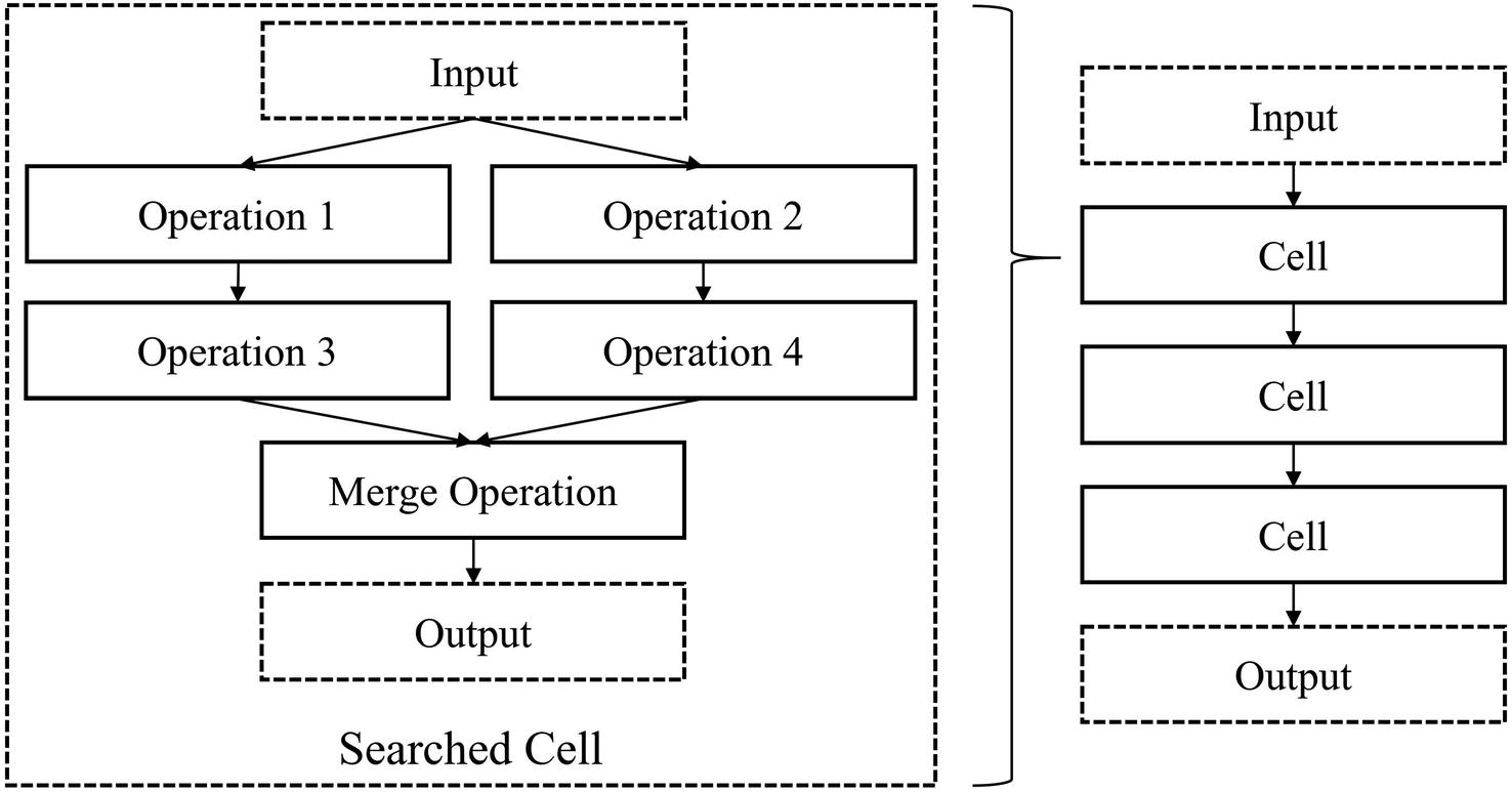
Cell-based neural network architecture representation. See NASNet for an example of a cell-based space
While the representative power of cell-based search spaces is significantly smaller than that of sequential representations (a network must be built with repeated segments to be efficiently represented cell-wise), it has yielded better performing architectures with shorter resource investment. Moreover, these learned cells can be rearranged, selectively chosen, and transferred to other data contexts and tasks.
Example recurrent neural network-based search strategy with a sequential information-based search space. This sort of design was used in early 2017 Neural Architecture Search work by Barret Zoph and Quoc. V. Le
Reinforcement learning is a commonly used search strategy for Neural Architecture Search. In the preceding example, for instance, the recurrent based neural network functions as the agent and its parameters function as the policy. The agent’s policy is iteratively updated to maximize the expected performance of the generated architecture.
Most search strategy methods face a problem: search space representations are discrete, not continuous, but gradient-based search strategies cannot operate on purely discrete problems. Thus, search strategies seeking to take advantage of gradients involve some operation to differentiate discrete operations.
Visualization of continuous relaxation in DARTS. Blue, green, and yellow connections represent potential operations that could be performed on blocks, like a convolution with a 5x5 filter size and 56 filters
Evolutionary search strategy methods don’t require this discrete-to-continuous mapping mechanism, however. Evolutionary algorithms repeatedly mutate, evaluate, and select models to obtain the best performing designs. While evolutionary search was one of the first proposed Neural Architecture Search designs in the early 2000s, genetic-based NAS methods continue to yield promising results in the modern context. Modern evolutionary search strategies generally use more specialized search spaces and mutation strategies to decrease the inefficiency often associated with evolution-based methods.
The simplest method to evaluate the performance of a search strategy is to train the proposed network architecture to completion and to evaluate the performance. This direct method of neural network evaluation suffices and is the most precise method of evaluation, but it is costly on computational and time resources. Unless the searching strategy requires relatively few models to be searched to arrive at a good solution, it’s usually infeasible to directly evaluate all proposed architectures.
Training on a smaller sampled dataset: Rather than training the model on the entire dataset, train proposed architectures on a smaller, sampled dataset. The dataset can be selected randomly or to be representative of different “components” of the data (e.g., equal/proportional quantities per label or data cluster).
Train a smaller-scaled version of the architecture: For architecture searching strategies involving predicting a cell-based architecture, the proposed architecture used for evaluation can be scaled down (i.e., fewer number of repeats or less complexity).
Predicting test performance curve: The proposed architecture is trained for a few epochs, and a time series regression model is trained to extrapolate out the expected future performance. The maximum of the extrapolated future performance is taken to be the predicted performance of the proposed architecture.
Demonstration of methods discussed for the search space, search strategy, and evaluation strategy components of NAS. Note that the discussed methods, of course, only cover some of modern NAS research
For more information on advances in NAS, see this chapter’s case studies, which detail three key advances in Neural Architecture Search.
Neural Architecture Search is currently a quite cutting-edge area of deep learning research. Many of the NAS methods discussed still require massive quantities of time and computational resources and are not suitable for general usage in the same way architectures like convolutional neural networks are. We will use Auto-Keras – a library that efficiently adapts the Sequential Model-Based Optimization framework for architecture optimization – for NAS.
Auto-Keras
There are many auto-ML libraries like PyCaret, H2O, and Azure; for the purposes of this book, we use Auto-Keras, an auto-ML library built natively upon Keras. Auto-Keras demonstrates the progressive disclosure of complexity principle, meaning that users can both build incredibly simple searches and run more complex operations.
To install, use pip install auto-keras.
Auto-Keras System
The Auto-Keras Neural Architecture Search system is one of very few easily accessible NAS libraries, as of the writing of this book – even state-of-the-art NAS designs are still too computationally expensive and intricate to be feasibly written into an approachable package.
Auto-Keras uses Sequential Model-Based Optimization (SMBO) , which was earlier presented as a formal framework for understanding Bayesian optimization.1 However, while generalized SMBO is designed to solve black-box problems, like the Tree-structured Parzen Estimator strategy used in Hyperopt, Auto-Keras exploits domain knowledge about the problem domain – neural network architectures – to develop more efficient SMBO components.
Simplified representation of the idea behind Gaussian processes – different fitted functions on sampled points and their associated probabilities. In practice, you probably won’t see a polynomial fit next to a sinusoidal fit in the same Gaussian process operation, but it is included for the sake of conceptual visualization
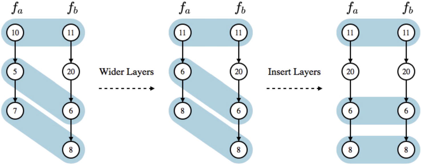
Figure showing morphing process used in the edit distance neural network kernel. First, the second and third layers in fa are widened to contain the same number of neurons as the corresponding layers in fb. Then, another layer is added to fa. Created by Auto-Keras authors
The edit distance neural network kernel allows for a quantification of similarity between neural network structures, which – roughly speaking – provides the necessary link from the discrete neural network architecture search space to the Euclidean space of the Gaussian process. Using the edit distance kernel and a correspondingly designed acquisition function, the Auto-Keras NAS algorithm is able to control the crucial exploit/explore dynamic – it samples network architectures with a low edit distance with respect to successful networks to exploit and samples network architectures with a high edit distance with respect to poorer performing networks to explore.
Auto-Keras trains each model to completion for some number of user-specified epochs (i.e., it uses a direct evaluation method rather than a proxy method), but its Bayesian character requires a fewer number of networks to be sampled and trained, provided the search space is well defined. In experiments carried out by Auto-Keras’ authors, Auto-Keras achieves a lower classification error than state-of-the-art network morphism and Bayesian-based approaches to Neural Architecture Search in the benchmark MNIST, CIFAR-10, and Fashion datasets.
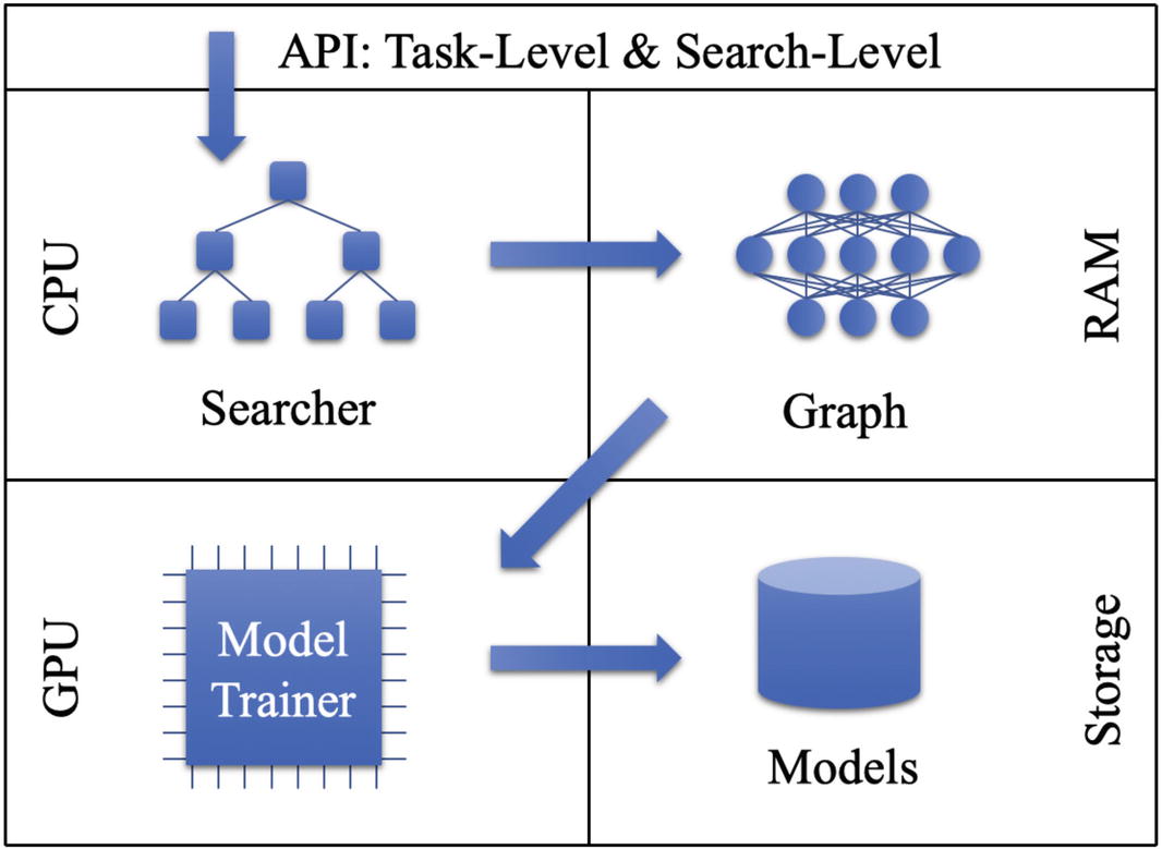
Auto-Keras’ API task-level and search-level operations in hardware. Created by Auto-Keras authors
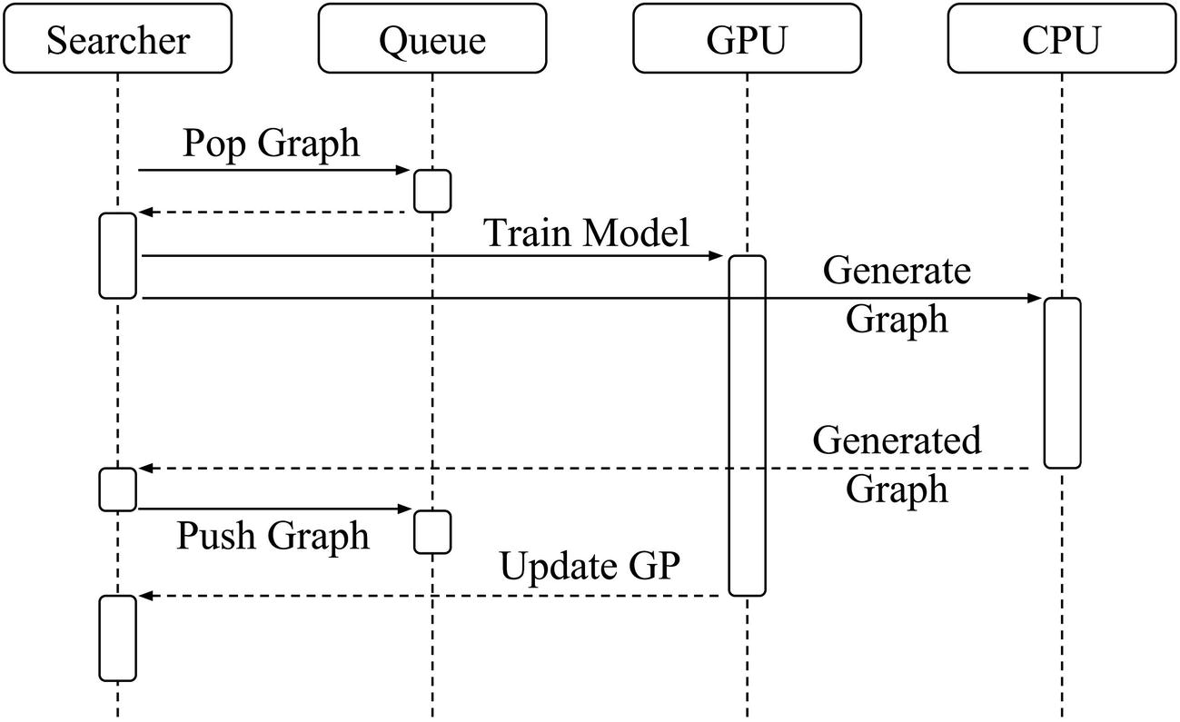
Auto-Keras’ system design – relationship between searcher, queue, GPU, and CPU usage. Proposed graphs are generated in CPU, kept in the queue, and trained in GPU
Both in its design and implementation, Auto-Keras is a key library in making Neural Architecture Search algorithms more efficient and accessible.
Simple NAS
- 1.
The input node : In this particular case, the input is an image input, so we use ak.ImageInput(), which accepts numpy arrays and TensorFlow datasets. For other input data types, use ak.StructuredDataInput() for tabular data (accepts pandas DataFrames in addition to numpy arrays and TensorFlow datasets), ak.TextInput() for text data (must be a numpy array or TensorFlow dataset of strings; Auto-Keras performs vectorization automatically), or ak.Input() as a general input method accepting tensor data from numpy arrays or TensorFlow datasets from all contexts. Using this last method comes at the cost of helpful preprocessing and linkage that Auto-Keras performs automatically when a context-specific data input is specified. These are known in Auto-Keras terminology as node objects. There is no need to specify the input shape; Auto-Keras automatically infers it from the passed data and constructs architectures that are valid with respect to the input data shape.
- 2.
The processing block : You can think of blocks in Auto-Keras as supercharged clumps of Keras layers – they perform similar functions as groups of layers, but are integrated into the Auto-Keras NAS framework such that key parameters (e.g., number of layers in the block, which layers are in the block, parameters for each layer) can be left unspecified and are automatically tuned. For instance, the ak.ConvBlock() block consists of the standard “vanilla” series of convolutional, max pooling, dropout, and activation layers – the specific number, sequence, and types of layers can be left to the NAS algorithm. Other blocks, like ak.ResNetBlock(), generate a ResNet model; the NAS algorithm tunes factors like which version of the ResNet model to use and whether to enable pretrained ImageNet weights or not. Blocks represent the primary components of neural networks; Auto-Keras’ design is centered around manipulating blocks, which allows for more high-level manipulation of neural network structure. If you want to be even more general, you can use context-specific blocks like ak.ImageBlock(), which will automatically choose which image-based block to use (e.g., vanilla convolutional block, ResNet block, etc.).
- 3.
The head/output block : Whereas the input node defines what Auto-Keras should expect to be passed into the input of the architecture, the head block defines what type of prediction task the architecture should be participating in by determining two key factors: the activation of the output layer and the loss function. For instance, in a classification task, ak.ClassificationHead() is used; this block automatically infers the nature of the classification head (binary or multiclass classification) and correspondingly imposes limits on the architecture (sigmoid and binary cross-entropy for binary classification vs. softmax and categorical cross-entropy for multiclass classification). If it detects “raw” labels (i.e., labels that have not been preprocessed), Auto-Keras will automatically perform binary encoding, one-hot encoding, or any other encoding procedure required to conform the data to the inferred prediction task. It’s usually best to make sure Auto-Keras does not need to make any drastic changes based on its inferences on your intent, however, as a precaution. Similarly, use ak.RegressionHead() for regression problems.
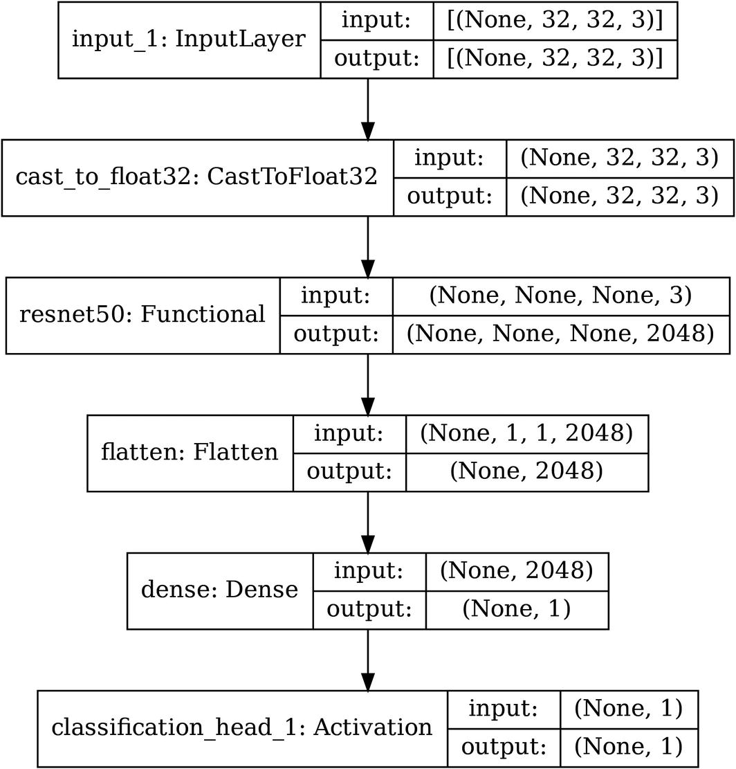
Simple input-block-head Auto-Keras architecture
For text data, use ak.TextBlock(), which chooses from vanilla, transformer, or n-gram text-processing blocks. Auto-Keras will automatically choose a vectorizer based on the processing block used. For tabular/structured data, use ak.StructuredDataBlock(); Auto-Keras will automatically perform categorical encoding and normalization. This will need to be followed by a processing block like ak.DenseBlock(), which stacks FC layers together.
Aggregating defined components into an Auto-Model and fitting
During the search, Auto-Keras will not only automatically determine which type of image-based block to choose but also various normalization and augmentation methods to optimize model performance.
You may also see some error messages printed when working with Auto-Keras for debugging purposes – as long as the code keeps on running, it’s generally safe to ignore the warnings.
Example sampled architecture of Auto-Keras model search
Unfortunately, such an approach – simply defining the inputs and outputs and letting Neural Architecture Search figure out the rest – is unlikely to yield good results in a feasible amount of time. Recall that every parameter you leave untuned is another parameter the NAS algorithm must consider in its optimization, which expands the number of trials it needs.
NAS with Custom Search Space
We can design a more practical architecture in terms of time to reach a good solution and computational burden by providing certain limitations on the search space using strategies that we know work.
General component-level design of image recognition models
- 1.
ak.ImageInput(), as discussed prior, is the input node.
- 2.
ak.ImageAugmentation() is an augmentation block that performs various image augmentation procedures, like random flipping, zooming, and rotating. Augmentation parameters, like whether to randomly perform horizontal flips or the range with which to select a factor to zoom or rotate, are automatically tuned by Auto-Keras if left unspecified.
- 3.
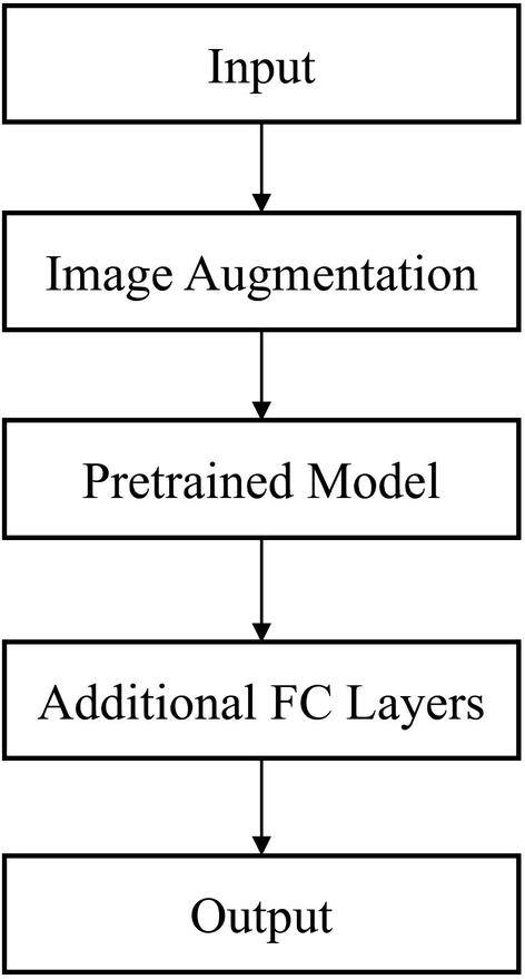
ak.ResNetBlock(), as discussed prior, is a ResNet architecture with only two parameters – which version of ResNet to use (v1 or v2) and whether to initialize with ImageNet pretrained weights or not. This serves as the pretrained model component of our image model design.
- 4.
ak.DenseBlock() is a block consisting of fully connected layers. If left unspecified, Auto-Keras tunes four parameters: the number of layers, whether or not to use batch normalization in between layers, the number of units in each layer, and the dropout rate to use (a rate of 0 indicates not to use dropout).
- 5.
ak.ClassificationHead(), as discussed prior, is the head block specifying the loss function to use and the activation of the last output layer.
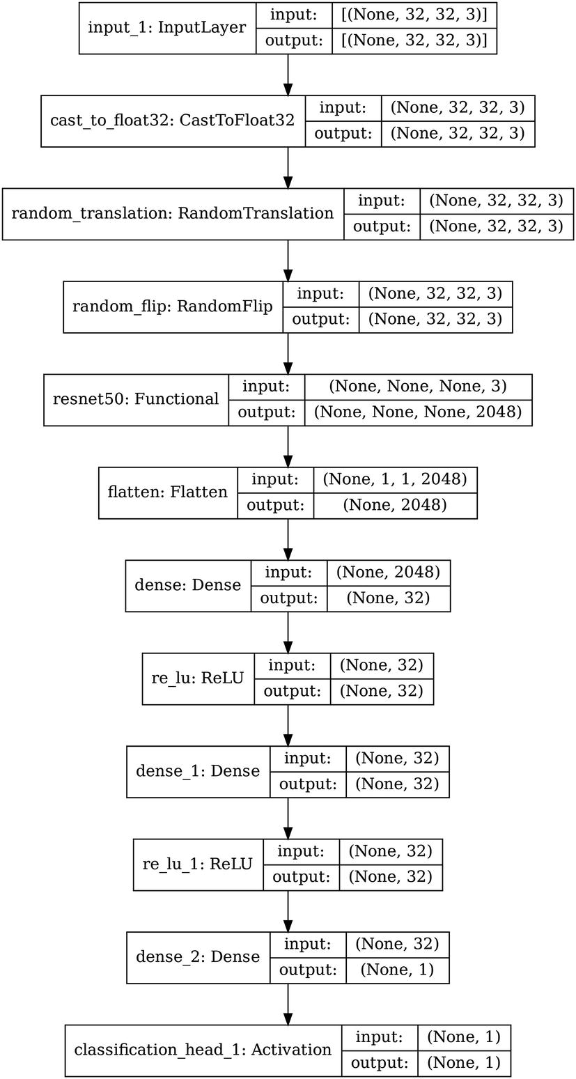
Defining an architecture with more complex custom search space, with all parameters specified
Defining an architecture with more complex custom search space, with only relevant parameters specified
The layers can then be aggregated into an ak.AutoModel (visualized in Figure 5-23) and fitted accordingly. By specifying a custom search space, you dramatically increase the chance that you will arrive at a satisfactory solution in less chance.
For text data, use ak.TextBlock(), use ak.Embedding() for embedding (can use GloVe, fastText, or word2vec pretrained embeddings as pretraining), and use ak.RNNBlock() for recurrent layers. For tabular/structured data, use ak.CategoricalToNumerical() for numerical encoding of categorical features in addition to standard processing blocks, like ak.DenseBlock().
Example sampled architecture of Auto-Keras model search
NAS with Nonlinear Topology
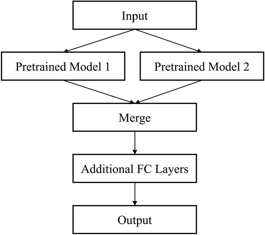
Component-wise plan for implementing a nonlinear topology in Auto-Keras
Building component-wise topologically nonlinear Auto-Keras designs
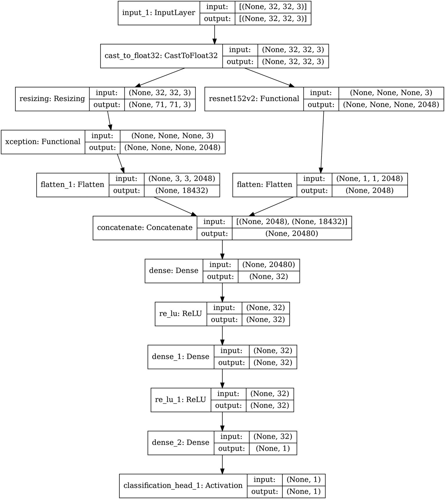
Example sampled architecture of Auto-Keras model search
Case Studies
These three case studies discuss three different approaches to developing more successful and efficient Neural Architecture Search systems, building upon topics discussed both in the NAS and the Bayesian optimization sections of this chapter. As pillars of the rapidly developing Neural Architecture Search research frontier, these case studies will themselves serve as the foundations upon future work in the automation of more powerful neural network architectures.
NASNet
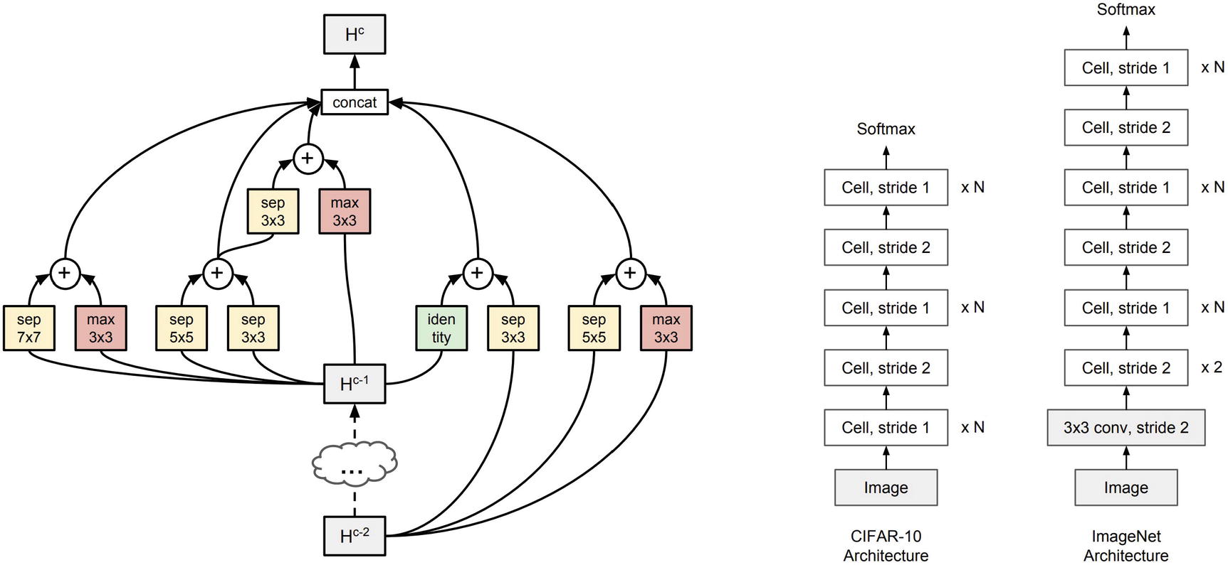
The NASNet search space , proposed by Barret Zoph, Vijay Vasudevan, Jonathon Shlens, and Quoc V. Le,2 is cell-based. The NAS algorithm learns two types of cells: normal and reduction cells. Normal cells make no change to the shape of the feature map (i.e., input and output feature maps have identical shapes), whereas reduction cells halve the width and height of the input feature map.
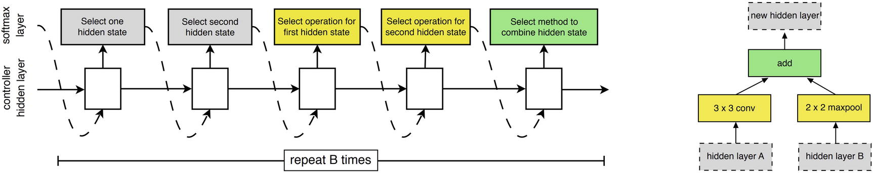
The generation of architectures via a recurrent model, which outputs hidden states, operations, and a merging method to select in the design of a cell
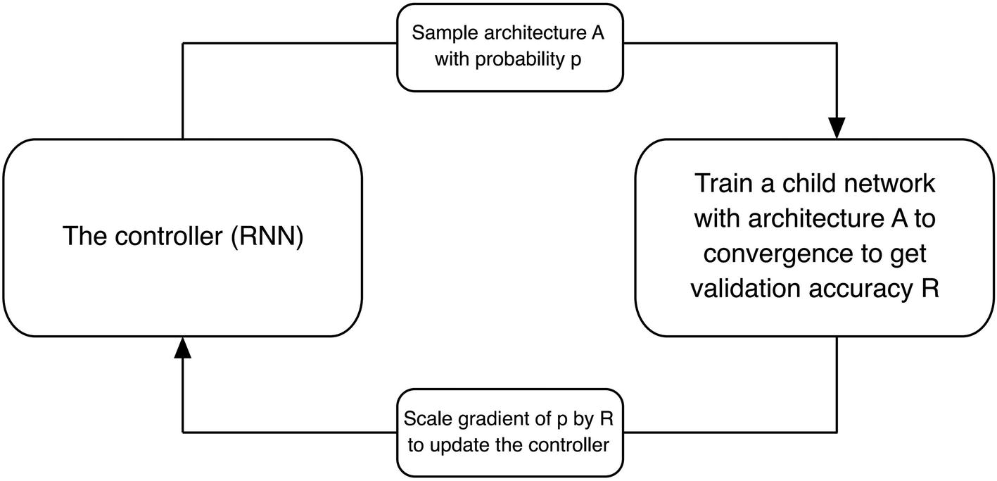
Relationship between the recurrent based controller and the proposed architecture (the child network). The controller is updated to maximize the validation performance of the child network. Created by NASNet authors
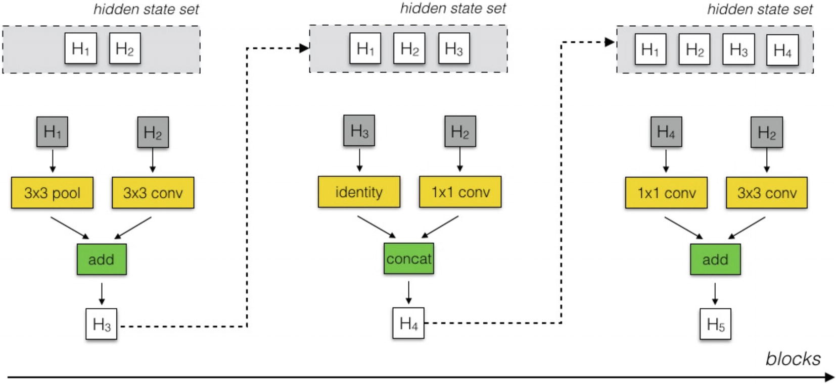
Example selection of hidden states and operations via recurrent style generation. Created by NASNet authors
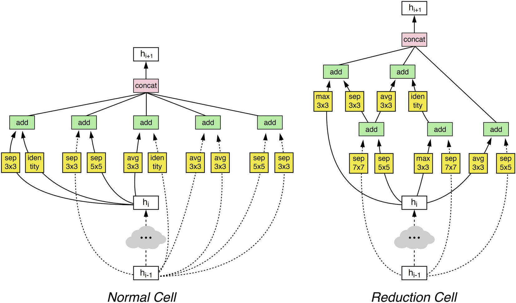
High-performing NASNet normal and reduction cell architectures on ImageNet. Created by NASNet authors
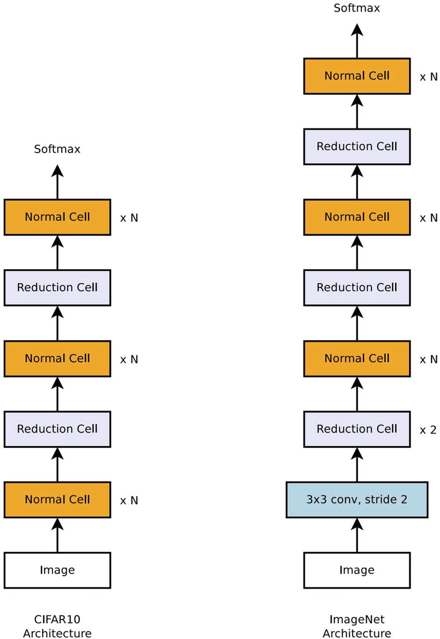
Stacking normal and reduction cells to suit a certain dataset image size. Created by NASNet authors
Performance of various sizes of NASNet (sizes determined by stacking different combinations and lengths of normal and reduction cells) against similarly sized models
Model | # Parameters | Performance | |
|---|---|---|---|
Top 1 Acc. | Top 5 Acc. | ||
Small-sized models – InceptionV2 – Small NASNet | 11.2 M 10.9 M | 74.8% 78.6% | 92.2% 94.2% |
Medium-sized models – InceptionV3 – Xception – Inception ResNetV2 – Medium NASNet | 23.8 M 22.8 M 55.8 M 22.6 M | 78.8% 79.0% 80.1% 80.8% | 94.% 94.5% 95.1% 95.3% |
Large-sized models – ResNeXt – PolyNet – DPN – Large NASNet | 83.6 M 92 M 79.5 M 88.9 M | 80.9% 81.3% 81.5% 82.7% | 95.6% 95.8% 95.8% 96.2% |
keras.applications.nasnet.NASNetMobile: 23 MB storage size with 5.3 m parameters.
keras.applications.nasnet.NASNetLarge: 343 MB storage size with 88.9 m parameters. (NASNet Large, as of the writing of this book, holds the highest ImageNet top 1 and top 5 accuracy of all keras.applications models with such reported metrics.)
See Chapter 2 on usage of pretrained models.
Even given NASNet’s advances in developing high-performing cell architectures, such results required hundreds of GPUs and 3–4 days of training in Google’s powerful laboratories. Other advances worked to build more computationally accessible search operations.
Progressive Neural Architecture Search
Chenxi Liu, along with other coauthors at Johns Hopkins University, Google AI, and Stanford University, proposes the Progressive Neural Architecture Search (PNAS).3 True to its naming, PNAS adopts a progressive approach to the building of neural network architectures from simple to complex. Moreover, PNAS interestingly combines many of the earlier discussed Neural Architecture Search methods into one cohesive, efficient approach: a cell-based search space, a Sequential Model-Based Optimization search strategy, and proxy evaluation.
Progressive Neural Architecture Search cell design. Left – high-performing PNAS cell design. Right – examples of how PNAS cell architectures can be stacked with different stride lengths to adapt to datasets of different sizes. Created by PNAS authors
PNAS makes use of a Sequential Model-Based Optimization search strategy, in which the most “promising” model proposals are selected for evaluation, in conjunction with a proxy evaluator.
The proxy evaluator, an LSTM, is trained to read an information sequence representing the architecture of a proposed model and to predict the performance of the proposed model. A recurrent based model was chosen for its ability to handle variable length inputs. Note that the proxy evaluator is trained on a very small dataset (the label – the performance of a proposed model – is expensive to obtain), so an ensemble of LSTMs trained on a subset of the data is used to support generalization and decrease variation. An RNN-based method’s predicted performance of candidate model architectures can reach as high as 0.996 Spearman rank correlation with the true performance rank.
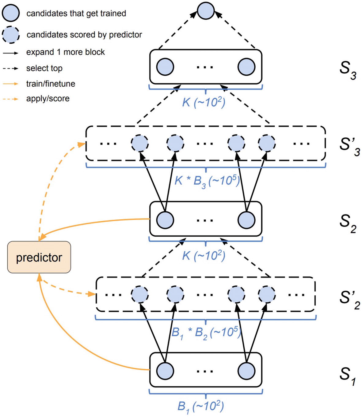
Visualization of the PNAS search and evaluation process. From S1 to S′2 trained cell architectures are expanded by one block. These generated cell architectures are evaluated via a proxy evaluator (labeled “predictor” in the visualization) and the top few are selected for training in S2. Created by PNAS authors. The performance of the generated architectures is used to update the proxy evaluator. The process repeats
The proxy evaluator functions as the surrogate function in Sequential Model-Based Optimization, used to perform sampling and updated using sampled results to be more accurate. Its progressive design allows for computational efficiency – if a smaller number of blocks per cell returns good performance, we have saved ourselves from needing to run through architectures with higher blocks per cell; even if a smaller number of blocks per cell does not yield good results, it functions as live training for the proxy evaluator.
Performance of PNAS against earlier work by Barret and Zoph in 2017, in which reinforcement learning is used to optimize a RNN to generate sequential representations of CNN architectures. Note that this is different from the closely related work by Zoph, Vasudevan, Shlens, and Le in 2018 on NASNet, which uses a cell-based representation. “# models trained on <method>” indicates the number of models the method trains to reach the listed corresponding performance. PNAS can reach almost a fivefold decrease in the number of models trained
Cells per Block | Top | Accuracy | # Models Trained by PNAS | # Models Trained by NAS |
|---|---|---|---|---|
5 | 1 | 0.9183 | 1160 | 5808 |
5 | 5 | 0.9161 | 1160 | 4100 |
5 | 25 | 0.9136 | 1160 | 3654 |
Efficient Neural Architecture Search
While proxy evaluation in Progressive Neural Architecture Search allows for quick prediction on the potential of a proposed model architecture and thus decreases the number of models that needs to be trained for good performance, the computational and time bottleneck in the process still remains in the training stage. Hieu Pham and Melody Y. Guan, along with Barret Zoph, Quoc V. Le, and Jeff Dean, put forth the Efficient Neural Architecture Search (ENAS) 4 method, which attempts to decrease the time needed to obtain accurate measurements on the performance of a candidate model by forcing weight sharing across all candidate architectures during training.
ENAS uses a similar reinforcement learning and recurrent based architecture generation model as the NASNet creators use, with one key difference: rather than predefining the “template” or “slots” of the cell and training the architecture generation model to identify which operations to “fill in” the “slots” with, in ENAS the controller model not only identifies which operations to choose but also how operations are connected.
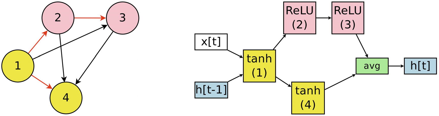
Left: “Fully connected” DAG with selected sub-graph shown in red. Right: example selected architecture based on sampled sub-graph
Recurrent model selection of sub-graphs from the “fully connected” DAG for the example model shown in Figure 5-30
The conceptual understanding of all sampled architectures as sub-graphs of the “super-graph,” “fully connected” DAG is crucial as the underlying basis of ENAS’ usage of weight sharing. The “fully connected” DAG represents a series of knowledge-based relationships between nodes; for maximum efficiency, the knowledge stored in the “fully connected” DAG’s connections should be transferred to selected sub-graphs. Thus, all proposed sub-graphs that contain the same connection will share the same value for that connection. Gradient updates performed on one proposed architecture’s connections are also performed identically on other proposed architectures with the same corresponding connections.
By sharing weights, proposed models can “learn from one another” by updating weights they have in common via the insights derived by another model architecture. Moreover, it serves as a rough approximation as to how models with similar architectures would have developed regardless under the same conditions.
This aggressive weight sharing “approximation” allows for massive quantities of proposed model architectures to be trained with much smaller computation and time consumption. Once the child models are trained, they are evaluated on a small batch of validation data and the most promising child model is trained from scratch.
Performance of ENAS against the results of other Neural Architecture Search methods. CutOut is an image augmentation method for regularization in which square regions of the input are randomly masked during training. CutOut is applied to NASNet and ENAS to increase performance of final architecture
Method | GPUs | Time (Days) | Params | Error |
|---|---|---|---|---|
Hierarchical NAS | 200 | 1.5 | 61.3 m | 3.63% |
Micro NAS with Q-Learning | 32 | 3 | – | 3.60% |
Progressive NAS | 100 | 1.5 | 3.2 m | 3.63% |
NASNet-A | 450 | 3–4 | 3.3 m | 3.41% |
NASNet-A + CutOut | 450 | 3–4 | 3.3 m | 2.65% |
ENAS | 1 | 0.45 | 4.6 m | 3.54% |
ENAS + CutOut | 1 | 0.45 | 4.6 m | 2.89% |
Key Points
In meta-optimization, a controller model optimizes the structural parameters of a controlled model to maximize the controlled model’s performance. It allows for a more structured search for the best “type” of model to train. Meta-optimization methods repeatedly select structural parameters for a proposed controlled model and evaluate their performance. Meta-optimization algorithms used in practice incorporate information about the performance of previously selected structural parameters to inform how the next set of parameters is selected, unlike naïve methods like grid or random search.
A key balance in meta-optimization is that of the size of the search space. Defining search space to be larger than it needs to significantly expands the computational resources and time required to obtain a good solution, whereas defining too narrow a search space is likely to yield results no different from user-specified parameters (i.e., meta-optimization is not necessary). Be as conservative in determining parameters to be optimized by meta-optimization (i.e., do not be overly redundant in your search space), but ensure that parameters allocated for meta-optimization are “wide” enough to yield significant results.
- Bayesian optimization is a meta-optimization method to address black-box problems in which the only information provided about the objective function is the corresponding output of an input (a “query”) and in which queries to the function are expensive to obtain. Bayesian optimization makes use of a surrogate function, which is a probabilistic representation of the objective function. The surrogate function determines how new inputs to the objective function are sampled. The results of these samples in turn affect how the surrogate function is updated. Over time, the surrogate function develops accurate representations of the objective function, from which the optimal set of parameters can be easily derived.
Sequential Model-Based Optimization (SMBO) is a formalization of Bayesian optimization and acts as a central component or template against which various model optimization strategies can be formulated and compared.
The Tree-structured Parzen Estimator (TPE) strategy is used by Hyperopt and represents the surrogate function via Bayes’ rule and a two-distribution threshold-based design. TPE samples from locations with lower objective function outputs.
Hyperopt usage consists of three key components: the objective function, the search space, and the search operation. In the context of meta-optimization, the model is built inside the objective function with the sampled parameters. The search space is defined via a dictionary containing hyperopt.hp distributions (normal, log-normal, quantized normal, choice, etc.). Hyperopt can be used to optimize the training procedure, as well as to make fine-tuned optimizations to the model architecture. Hyperas is a Hyperopt wrapper that makes using Hyperopt to optimize various components of neural network design more convenient by removing the need to define a separate search space and independent labels for each parameter.
- Neural Architecture Search (NAS) is the process of automating the engineering of neural network architectures. NAS consists of three key components: the search space, the search strategy, and the evaluation strategy. The search space of a neural network can be represented most simply as a sequential sequence of operations, but it’s not as efficient as a cell-based design. Search strategies include reinforcement learning methods (a controller model is trained to find the optimal policy – the parameters of the controlled model) and evolutionary designs. Methods like DARTS map the discrete search space of the neural network into a continuous, differentiable one. Evaluation of sampled parameters can take the form of direct evaluation or via proxy evaluation, in which the performance of the parameters is estimated with fewer resources at the cost of precision.
The Auto-Keras system uses Sequential Model-Based Optimization, with a Gaussian process-based surrogate model design and the edit distance neural network kernel to quantify similarity between network structures. Moreover, Auto-Keras is built with GPU-CPU parallelism for optimal efficiency. In terms of user usage, Auto-Keras employs the progressive disclosure of complexity principle, allowing users to build both incredibly simple and more complex architectures with few lines of code. Moreover, because it follows Functional API-like syntax, users can build searchable architectures with nonlinear topologies.
In the next chapter, we will discuss patterns and concepts in the design of successful neural network architectures.