
4
Invisibility
Pascal LEFÈVRE1, Philippe CARRÉ1 and David ALLEYSSON2
1 XLIM, CNRS, University of Poitiers, France
2 LPNC, Grenoble Alpes University, Savoie Mont Blanc University, CNRS, Grenoble, France
In this chapter, we intend to discuss the different strategies to ensure the invisibility of a message embedded in a color image. The term “invisibility” here relates to the visual aspect. For grayscale images, many solutions have been developed, attempting to take into account the modeling of the human visual system (HVS) in order to limit degradation. However, the extension of these solutions to color images often proposes an adaptation of the strategies dedicated to grayscale images, configured by a wise choice of a color component. Even when a dedicated approach to color is introduced (such as through the use of quaternion formalism), the same challenge is present; in other words, the correct choice of the direction of the insertion color. In this chapter, we discuss these aspects and we conclude by introducing a method configuring this choice of color direction, depending on psycho-visual considerations.
4.1. Introduction
In this chapter, we focus on the watermarking of color images that involves the current framework of modern watermarking algorithms. In this book, different watermarking methods for color images are presented, however, many of them proceed in a similar way: selecting a chromatic or achromatic channel in order to have only one scalar detail to manipulate per pixel, and then a watermarking strategy is applied from the techniques that are defined for grayscale images. Keeping this in mind, the first color solutions (Kutter et al. 1997; Yu et al. 2001) suggested watermarking the blue component in order to minimize the visual impact in the modified image. In fact, it is well known that modifications of the blue component will be less visible. As is often the case, this stronger invisibility will go hand in hand with a greater fragility. Continuing this strategy, but looking for other compromises, different methods introduced the modification of the luminance component (Voyatzis and Pitas 1998) or the saturation component (Kim et al. 2001), which allowed them to be more robust, but generally had greater distortion during insertion. In fact, the modification of a component like luminance leads to visible damage (if not, the insertion force must be very small).
Since then, several propositions for color have been made, but the majority of them use strategies that we consider “grayscale”, or scalar methods, as they only use one component. Therefore, the challenge is always to choose this component well. Through the choice of a single component, the risk is that the concept of color is not taken into account, or more precisely, the vector dimension of the information is not used. This generally leads, from the choice of the component, to favoring robustness or invisibility. In addition, poor choice of the component does not make it possible to obtain an optimal invisibility for the human visual system (HVS). In order to take into account this information that is translated by three values, certain methods tend to treat each color component independently of one another and again apply a grayscale method on each component (e.g. Dadkhah et al. (2014)). These methods, therefore, treat the color components independently. However it is now well-established that the color components are correlated, and so these marginal approaches do not allow us to obtain an optimal invisibility for the HVS.
This is why, in order to maximize the invisibility/robustness compromise, approaches have appeared that consider color information in a more global way. For example, Abadpour and Kasaei (2008) used the information obtained from the projections of a main component analysis. Other contributions suggest the use of transformed domains that are adapted to color, such as the quaternion discrete cosine transform (Li et al. 2018) or specific manipulations (Parisis et al. 2004). There are also vector methods on wavelet coefficients that are calculated from the three RGB planes or from another space, which will try to limit the visual degradation by setting the insertion force in the domain of the transform to using, for example, the concept of Just Noticeable Difference (JND) (Chou and Liu 2010) that we describe below. In this case, the algorithm does not take into account the perceptual dimension of the color during the decomposition, but in the configuration of the modification. To integrate the concept of HVS, the works proposed by Chareyron et al. (2004) allow the insertion of a 2D mark in the chromatic xy plane. Their approach is based on a histogram manipulation offered by Coltuc and Bolon (1999). To improve the invisibility of the mark, the color distances corresponding to the distortions are calculated in the L*a*b* color space (Chareyron and Trémeau 2006). As we have mentioned, in order to introduce HVS modeling, the concept of JND has been used for a long time. JND initially makes it possible to assess the damage linked to a watermarking strategy, but this concept remains an open problem with regard to digital models, in particular without preconception about the content of the image. JND is used in grayscale approaches, particularly for insertion in the transform domain (DCT). For example, Watson’s perceptual model (Watson 1993), proposed in 1993, makes it possible to visually optimize the quantization DCT matrices for a given image during its compression due to adaptations of contrast and luminance. These works were incorporated into digital watermarking by Li and Cox (2007) and also by Hu et al. (2010) in order to minimize insertion noise. However, as we can see, these works remain in the domain of grayscale images, and inclusion of color according to this strategy remains more unreliable (Chou and Liu 2010; Wan et al. 2020). Some of the literature dedicated to watermarking color images uses the concept of quaternions. However, as we will show in this chapter, the representation space remains configured by choices of chromatic direction controlling this question of invisibility. The quaternionic context for color image watermarking is discussed in section 4.3.
A more detailed understanding of the processing of color by the HVS would improve the invisibility of a mark. To illustrate this point, this chapter discusses a vector quantification method (section 4.2), associated with a biological model of HVS photoreceptors to be able to insert information into color images. The model studied is based on a psychovisual approach (section 4.4), making it possible to understand the HVS’s perception of color differences (work introduced by Alleysson and Méary (2012)). We then adapt it to digital watermarking in order to minimize psychovisual distortions. We then detail the different steps of a robust watermarking scenario for color images, as well as the algorithms used to adapt the QIM Lattice (LQIM) method.
First of all, in order to illustrate the issue of color watermarking, we propose a general framework in section 4.2, making it possible to manipulate the color within the framework of a watermarking algorithm.
4.2. Color watermarking: an approach history?
As we have said, different approaches have been offered, based on the use of color space suitable for the insertion of a watermark, that is invisible to the naked eye. As a reminder, one of the first approaches involved inserting a mark in the blue component of the RGB space because the HVS is less sensitive to distortions in this channel (Kutter et al. 1997; Yu et al. 2001).
It is therefore a question of constructing a vector modification procedure, and to illustrate this, we choose a modification by quantization. Note that the discussion conducted in this framework by quantization can be generalized to other modification strategies and to simplify the understanding of the impact of modification, we intend to describe the process in the spatial domain.
4.2.1. Vector quantization in the RGB space
Vector quantization allows us to insert information about the values of a color pixel (three dimensions). It can be considered as a quantization on a line segment generated by a direction vector (Figure 4.1).
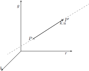
Figure 4.1. Quantization in the RGB color space on an oriented line by a direction vector u
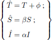
Let P be a value of a color pixel. The result of quantization, denoted by P′ is defined by:
with uP, a direction vector, and s =< P, uP >, the canonical scalar product of P by uP.
This equation modifies the color P according to s along the direction axis uP. Depending on the color P on which the vector quantization is applied, the color distortion perceived by the HVS is different.
At the detection stage, the value to be estimated is s′. If the color is modified after the insertion of a watermark, we have:
with P″, a color modified after inserting information, and uP″, its associated direction vector. We then have a decoding condition on the direction vectors: it is necessary that the direction vectors uP and uP″ are close enough to have a good estimate of s′.
Assuming we are in a case where detection is possible, that is, the color difference P″ − P ′ is small enough, we then have:
4.2.2. Choosing a color direction
The main differences between color specific watermarking methods are as follows:
- – the insertion method (as for grayscale approaches);
- – the choice of “color” information that will carry the message.
Whether the approaches are direct (use of a color channel), indirect (change of spaces) or even adapted (construction of a specific transform), in general, they can be modeled by the insertion of a message following a certain direction in the RGB cube. Therefore, the aim is to find a direction that minimizes the color quantization noise for the HVS.
To start with, we will study a basic approach that involves choosing a fixed insertion direction for the whole image. This approach illustrates the influence of this choice of direction when there is no local adaptation. If we randomly choose a direction vector constant for every color in the image, the HVS detects color distortions very easily (Figure 4.2(b)) since the choice of direction introduces colors that are not relevant to the content of the image.
We can reduce the detected quantization noise by using a direction that is judiciously fixed for the whole image; this is the case for a large number of algorithms in this book. A direction vector that limits color distortions is vector ![]() , which represents the gray level axis in the RGB space. An example is illustrated in Figure 4.2(c). In fact, compared to Figure 4.2(b), for the same level of modification, we no longer see false colors appearing.
, which represents the gray level axis in the RGB space. An example is illustrated in Figure 4.2(c). In fact, compared to Figure 4.2(b), for the same level of modification, we no longer see false colors appearing.
However, these first results are not satisfactory in terms of watermarking invisibility. Depending on the color we modify, the detection of quantization noise is different, we have to introduce a so-called adaptive approach. For each color P, we must determine which direction vector choice minimizes the quantization noise, in the sense of the HVS. Figure 4.2(d) shows an example of a watermarked image with an adaptive approach that we will describe in section 4.4.5. We can see that the quantization noise is less visible. However, on closer inspection, we observe a slight colored noise in the homogeneous (or non-textured) areas of the image, such as the green and brown background; the local context of the image is also important.
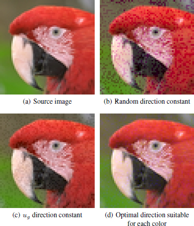
Figure 4.2. Example of inserting a mark with different approaches and direction vectors with equivalent digital distortion (overall, the signal to noise ratio is equivalent for the three images). The image used is a cropped version of the image kodim23.png from the Kodak Image Database (available at: http://r0k.us/graphics/kodak/kodim23.html)
As we suggested in the introduction, approaches using a more evolved representational space must address the same question: which is the best direction? To show this, we intend to recall the context of image watermarking according to quaternionic transforms.
4.3. Quaternionic context for watermarking color images
Quaternions can be a tool to manipulate color, which explains the different works offering quaternion-based watermarking (Bas et al. 2003; Tsui et al. 2008). In this section, we offer a few introductory elements on the tool.
4.3.1. Quaternions and color images
The quaternion algebra is algebra, ![]() , of dimension 4 over
, of dimension 4 over ![]() , made up of the elements of the form:
, made up of the elements of the form:
with the real number S(p), the scalar part, and the vector V (p), the vector part of the quaternion q.
All the usual geometric operations of ![]() 3 can be found when we limit the operations of quaternions to the set
3 can be found when we limit the operations of quaternions to the set ![]() 0 of pure quaternions (if q = (S(q), V (q)) then S(q) = 0). Let q1 and q2 be two pure quaternions representing the vectors V1 and V2 of
0 of pure quaternions (if q = (S(q), V (q)) then S(q) = 0). Let q1 and q2 be two pure quaternions representing the vectors V1 and V2 of ![]() 3, respectively, so:
3, respectively, so:
- 1) q1 + q2 = V1 + V2;
- 2) q1.q2 = V1.V2;
- 3) q1q2 = −V1.V2 + V1 ⌃ V2.
Note that the quaternionic product of two pure quaternions contains, in its real part, the scalar product of the two vectors represented, and, in its imaginary part, the cross product. This result is present in some uses of quaternions for color images.
The algebra is provided with the product:
where V (p).V (q) (respectively, V(p) × V (q)) denotes the scalar product (respectively, mixed or vectorial) of two vectors V (p) and V (q) of ![]() 3.
3.
The algebra ![]() is associative but not commutative.
is associative but not commutative.
We can find the so-called Hamilton form q = q0 + iq1 + jq2 + kq3, of quaternion q, by writing: i = (0, 1, 0, 0), j = (0, 0, 1, 0) and k = (0, 0, 0, 1). The calculation rules then become:
We find a vocabulary that is similar to that of complex numbers. The conjugate ![]() of a quaternion q is defined by:
of a quaternion q is defined by: ![]() = q0 − iq1 − jq2 − kq3. Any quaternion q that is not zero accepts an inverse, called q−1 = q/|q|2, where
= q0 − iq1 − jq2 − kq3. Any quaternion q that is not zero accepts an inverse, called q−1 = q/|q|2, where ![]() . The positive real number
. The positive real number ![]() is the magnitude of q, denoted |q|. As for complex numbers, it is possible to define combined quaternions (if q = (S(q), V (q)) then S(q)2 + ‖V(q)‖2 = 1).
is the magnitude of q, denoted |q|. As for complex numbers, it is possible to define combined quaternions (if q = (S(q), V (q)) then S(q)2 + ‖V(q)‖2 = 1).
Since a color contains only three components in the RGB space, it has been suggested that we describe the color information on the imaginary part of the quaternions (Sangwine 2000):
The color of a pixel of an image f at spatial coordinates (m, n) is then coded in the following way:
with fr[m, n], fv[m, n] and fb[m, n] as the red, green and blue components of the pixel of coordinates (m, n), respectively. This is how, in the vast majority of quaternion based color watermarking algorithms, the information is modified.
Consider a pixel color f[m, n] = (fr[m, n], fv[m, n], fb[m, n]) coded by a pure quaternion q:
We want to extract the colorimetric coordinates (intensity, hue and saturation). First we need to define a vector µ (pure unitary quaternion) representing the axis of intensities. The intensity I of q is the projection of this on µ:
This axis is generally defined as the grayscale axis, so ![]() , but in a watermarking strategy a choice for this direction µ can be more adaptive. Following this idea, we can generalize the operations for manipulating color information through the quaternion formalism (Carré et al. 2012):
, but in a watermarking strategy a choice for this direction µ can be more adaptive. Following this idea, we can generalize the operations for manipulating color information through the quaternion formalism (Carré et al. 2012):
with the result:
These few simple operations allow us to illustrate the first links between quaternions and color. We note that, again, the central element to all modifications is the definition of an axis µ, around which the different transforms will be configured. This is the case for quaternionic watermarking algorithms. However, most of them use a transformed domain, particularly a frequency domain.
4.3.2. Quaternionic Fourier transforms
Quaternionic Fourier transforms (QFT) were introduced in the context of color images by Sangwine and Ell (2001) in order to generalize the complex Fourier transform for color images. There are several versions of quaternionic Fourier transforms with different aims, particularly because the quaternionic product is not commutative. Sangwine offers a color version by adding a direction that is characterized by a pure unitary quaternion, to the expression of the exponential µ (Ell and Sangwine 2006). Most often, in order to avoid favoring any color for the spectral analysis, the neutral quaternion µ = µgris = (i + j + k)/![]() is chosen and corresponds to the achromatic axis of the RGB space. The definition is as follows:
is chosen and corresponds to the achromatic axis of the RGB space. The definition is as follows:
It is possible to place the exponential to the right of the function f. We then obtain the definition of another Fourier transform since the quaternionic product is not commutative.
Different authors have looked to give an interpretation to the information described by the spectrum coefficients. We can identify three main approaches:
- – describe the quaternion spectrum with the exponential representation (Assefa et al. 2010);
- – break down each spectral coefficient into two parts, one simplex and one perplex, in order to separate the luminosity data from the chrominance data (Sangwine and Ell 2001);
- – carry out an analysis of elementary atoms (Denis et al. 2007).
This frequency information present in the quaternionic spectrum is especially used in digital image watermarking (Bas et al. 2003). To analyze watermarking in quaternion space, we introduce the Cayley–Dickson construction, which allows the separation of data into a luminosity part and a chromaticity part (Ell and Sangwine 2000). This rewriting has made it possible to analyze the transformations carried out with the quaternions through a “colormetric” view. We have seen that a quaternion can be considered as a vector of the base (e, i, j, k) with e = 1, the real unitary vector:
with a, b, c, d as any four real numbers of which a is the real part and (b, c, d) is the imaginary part.
We can choose another base, for example (e, µ, ν, µν) with µ and ν, two pure unitary orthogonal quaternions. Their product µν is also a pure and orthogonal quaternion to the other vectors of the base. We can write q in this base:
with, for example, the real number qe = q.e defined by the scalar product and which therefore corresponds to the projection of q on e.
Likewise, we can calculate qµ = q.µ, qν = q.ν and qµν = q.µν of real numbers.
Notice that it is possible to regroup the quaternion q in two isomorphic subspaces in ![]() . In fact, the first block (qe, qµ) corresponds to the real part and the projection term on µ, the remainder being expressed in the plane (ν, µν), which is the plane perpendicular to µ. The quaternion can therefore be written as:
. In fact, the first block (qe, qµ) corresponds to the real part and the projection term on µ, the remainder being expressed in the plane (ν, µν), which is the plane perpendicular to µ. The quaternion can therefore be written as:
with q‖ = qee + qµµ and q⊥ = qνe + qµνµ, q‖ being the parallel part to µ and q⊥ the perpendicular part.
In the case of pixel color manipulation, two pure quaternions are used for this decomposition: the first vector µ is, for example, the gray axis in the cube RGB:
The second is the axis perpendicular to µ in the direction of the red color (pointing out axis i):
since the red is used as a reference for a zero-value hue in the chromticity plane.
In this case, when a color image is divided into parts parallel and perpendicular to µ, it seems that this decomposition allows the separation of luminosity data on the parallel part, and chromatic data on the part perpendicular to µ. We find the classic representation associated with luminance–chrominance spaces.
When a watermarking algorithm suggests using the quaternion space to carry out the insertion of a message, especially in the transformed domain, in many cases the operation can be interpreted through the Cayley–Dickson representation. This results in a modification of the color pixels in one of the directions: the impact of the modification will therefore depend on the explicit or implicit choice of the µ axis. Although the approach uses a more complex model which seems to take the color into account, the algorithm remains configured by a wise choice of insertion color direction.
In section 4.4, we propose to discuss a psychovisual model that makes the choice of direction as adaptive as possible, that is, we show how to determine the optimal direction vectors for any RGB color.
4.4. Psychovisual approach to color watermarking
4.4.1. Neurogeometry and perception
Understanding how humans perceive color differences can allow us to minimize insertion color distortions perceptually; in other words, to improve watermark invisibility. To achieve this objective, we need a color discrimination model. This model would be three dimensional, due to the human trichromy, and should mimic the representation of light by the cones of the human retina for their spectral sensitivities as well as their intensity encoding dynamics.
This type of model, known as neurogeometry, was suggested in the context of the perception of shapes based on achromatic data. A detailed description of the construction of forms by the primary visual cortex is given in Petitot (2003, 2008). Few other contributions have considered neurogeometry in the context of color vision (Koenderink et al. 1970; Zrenner et al. 1999; Alleysson and Méary 2012), and even less in the application context of color watermarking.
In this section, we limit our study to the modeling part and its application for color watermarking: more precisely, we use a chromatic discrimination ellipsoid model based on the Naka–Rushton law of photoreceptor dynamics.
A simple and effective way to model color discrimination data involves considering color discrimination to be a nonlinear operation in a three-dimensional Euclidean vector space φ ≅ ![]() 3. The space has the standard scalar product xy = x1y1 + x2y2 + x3y3, where x = [x1, x2, x3] and y = [y1, y2, y3] are two vectors in
3. The space has the standard scalar product xy = x1y1 + x2y2 + x3y3, where x = [x1, x2, x3] and y = [y1, y2, y3] are two vectors in ![]() 3 linked to two points, M and N, as
3 linked to two points, M and N, as ![]() and
and ![]() with O, the origin of vectorial space associated with ϕ. The magnitude of a vector x is given by
with O, the origin of vectorial space associated with ϕ. The magnitude of a vector x is given by ![]() . The distance between x and y is given by d(x, y) = ‖x − y‖.
. The distance between x and y is given by d(x, y) = ‖x − y‖.
Assume that this space φ is a physical space in which the HVS maps another representation ψ, marked by a quadratic form q(x) = xtGx where G is a symmetrical positive definite matrix representing the metric brought about by the nonlinearity of the HVS. This quadratic form defines a new form for vectors in the visual space, such as ![]() , and a scalar product balanced such that:
, and a scalar product balanced such that:
In this model, we assume that the HVS maps the physical space of light φ and the perceptual space ψ. An equal discrimination contour is represented by a circle on an isoluminant surface and the physical space is a space in which this constant discrimination circle in ψ corresponds to an ellipse in φ. The mapping function between these spaces is given by the neuronal function. This model is illustrated in Figure 4.3. In this figure, we assume that the HVS is a nonlinear function f between the flat physical space of light φ and the curved space of perception ψ. In this section, we use a modification of the Naka–Rushton transduction equation to account for visual nonlinearity.
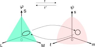
Figure 4.3. Relationship between physical space ϕ and perceptual space ψ
For the sake of generality, we must consider that G depends on the physical stimulus x and on the adaptation state of the observer x0, so we write G(x, x0). The question to be solved for a color discrimination space is to find the relationship between the nonlinearity brought about by the HVS, and the shape of the metric G(x, x0). One way to clarify this relationship is to fix the adaptive nonlinearity function. This cannot be done in general, but we assume that the nonlinearity of the HVS operates on each color channel separately and that it is parametric with an adaptation parameter, which modifies the curve of the nonlinearity.
4.4.2. Photoreceptor model and trichromatic vision
Based on this principle, we introduce a three-dimensional construction of an HVS trichomatic model (Alleysson and Méary 2012).
An HVS is a complex system that adapts according to environmental conditions, and it is no surprise that color vision is a nonlinear, adaptive phenomenon.
Assume for now that x is a physical one-dimensional variable corresponding to light entering the eye. y = f(x, x0) is the transformation of this variable by the HVS according to an adaptation factor x0.
We define f as a simplification of the Naka–Rushton function, which checks the transduction of light by the photoreceptor (Alleysson and Hérault 2001):
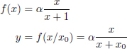
where y is the level of transduction. In other words, y represents the electric response of a cone as a function of x, the level of excitation of the cone produced by light and x0, the state of adaptation.
x0 is modified according to the average excitation level of the photoreceptor. Equation [4.8] represents the behavior of the photoreceptor according to two constants, α and x0, set by the environmental conditions and the HVS state. In fact, the adaptation process of a photoreceptor is only partially understood and this model is probably a simplification.
We assume that this is the nonlinear, adaptive function of equation [4.8], which matches physical space to perceptual space. The function saturates α when x → ∞ and x0 gives the half-maximum of the curve. The function’s curve changes according to x0. A low x0 gives a high curvature, while a high x0 gives a low curvature. This nonlinear function is shown in Figure 4.4.
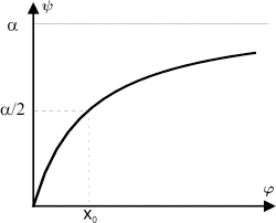
Figure 4.4. Nonlinear function of perception
Therefore, considering the three-dimensional space of the physical colors φ, we establish the link between the physical and perceptual space by:
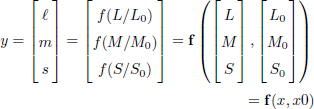
where x = [L, M, S] and x0 = [L0, M0, S0] are coordinates of the physical stimulus in the space φ, and the adaptation of the observer expressed as a parameter in the space φ, respectively.
Here, we implicitly assume, without losing generality, that the coordinates in the space φ correspond to the responses of cones L, M and S. L, M and S are then the encoding of the physical stimulus x by the HVS, suitable for x0.
To summarize, the human retina possesses three types of photoreceptors, which are cones L, M and S. The responses of each of these cones are processed by a nonlinear parametric function that defines the perceptual variables. For each color channel, there are two parameters, α and x0:
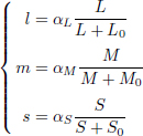
where the parameters αL, αM and αS are gains on the respective components L, M and S. The constants L0, M0 and S0 are the adaptation states of the respective cones.
In the trichromatic model of color vision, it is possible to find a three-dimensional construction of color discrimination with the photoreceptor model described above. In the space of transduction lms, pairs of points separated by the same distance have the same level of perception of the color difference. When these pairs are converted in the excitation space LMS, Euclidean distances are no longer equal even though the same level of perception is maintained.
This distortion phenomenon can be better observed by constructing a sphere centered at Plms = (lc, mc, sc) in the space lms defined as:
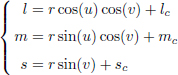
with r, the radius of the sphere, −π ≤ u ≤ π and −π/2 ≤ v ≤ π/2.
By converting the sphere in the space LMS, we get a volume ![]() defined by:
defined by:
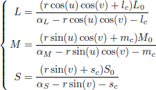
The distances between the center of the volume Plms and the points on the surface of the volume are therefore constant:
with a constant radius of r.
Note that r is no longer constant in the case of the volume ![]() of center PLMS = f−1(Plms).
of center PLMS = f−1(Plms).
4.4.3. Model approximation
We then need to explain how to calculate G(x, x0), the metric from f. To do this, we consider that in the perceptual space ψ, an equal discrimination contour around a point (ℓc, mc, sc) is a sphere S with radius 1. So we write:
As we have seen, in the physical space, the resulting surface is given by the linear approximation of the nonlinearity ![]() around xc. As we can consider dy to be very small, it is given by the Jacobian of f:
around xc. As we can consider dy to be very small, it is given by the Jacobian of f:
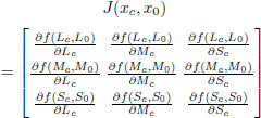
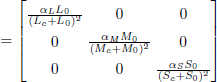
This approximation makes it possible to establish a direct correspondence between dy = [ℓ − ℓc, m − mc, s − sc] and dx = [L − Lc, M − Mc, S − Sc]:
As we have mentioned, a circle in perceptual space ψ corresponds to an ellipse in physical space φ expressed as:
G is equal to:
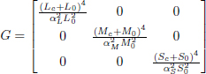
We see that, from a color defined by coordinates (Lc, Mc, Sc), we have two groups of parameters in this transformation, (L0, M0, S0) and (αL, αM, αS).
4.4.4. Parameters of the model
To use this model, the constants L0, M0 and S0 and the gains αL, αM and αS can be calculated using MacAdam ellipses (MacAdam 1942) (Figure 4.5).
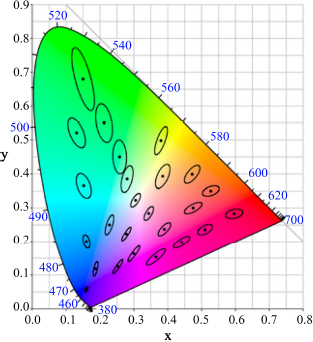
Figure 4.5. MacAdam ellipses in the luminance plane of the color space xyY, 1931. Ellipses are 10 times larger than their original sizes
If we want to calculate these parameters from the MacAdam ellipses, we have to first transform the MacAdam measurement made in the CIE-xyl space into space LMS. To do this, we use the following transformation:
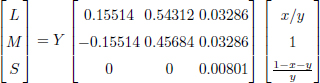
With this transformation of (x, y, l) into (L, M, S) and with the parameter (αL = 1665, αM = 1665, αS = 226), (L0 = 66, M0 = 33, S0 = 0.16), it has been shown that this allows a good reconstruction of MacAdam ellipses (Figure 4.6) (Alleysson 1999).
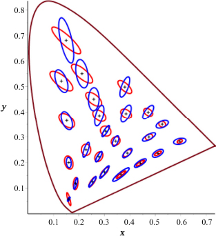
Figure 4.6. The ellipses obtained from the psychovisual model almost correspond to the MacAdam ellipses after an optimal choice of constants (Alleysson 1999)
4.4.5. Application to watermarking color images
In section 4.4.4, we introduced a color vision model to develop a less visible method of watermarking. In the color space LMS, we constructed ellipsoids that concretely illustrate how to control psychovisual distortion while ensuring satisfactory robustness.
In fact, the idea of psychovisual distorsion represents the perception of the color difference on insertion, as opposed to digital (Euclidean) distortions obtained with metrics such as the PSNR. As psychovisual distortions better describe the invisibility of the watermark for the HVS than digital distortion measurements, the theory is that it becomes possible to obtain a better compromise between invisibility and robustness: for the same level of psychovisual distortion, there are different levels of digital distortion, depending on the insert setting, and choosing maximum digital distortion improves robustness.
In this section, we intend to remove, for each color pixel P, the direction vector uP which has the largest magnitude in its ellipsoid.
4.4.6. Conversions
Here we give the color space conversion matrices to work from XYZ and LMS psychovisual spaces to RGB space. The transformations are chosen according to the 1931 CIE standard1. The conversion between color spaces is represented by the following matrices:
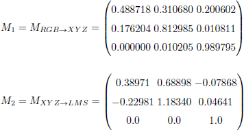
Let PRGB, PXYZ and PLMS be the color pixels in their respective RGB spaces, XYZ and LMS. We have:
In section 4.2, we have seen that the choice of a direction vector has an enormous impact on the invisibility of a watermark. When we choose a fixed direction for all the colors, we note strong psychovisual distortions in certain areas of the image. However, invisibility is greatly improved when the best direction vector is chosen for each color pixel. Since we assume that the psychovisual distortions are the same for all the elements of ψ, we can choose the point furthest away from P, indicated by Pf, to allow the maximum numerical distortions authorized during integration in order to reinforce robustness. The direction vector uP is defined such that ![]() .
.
Note that ℰ is the set of points belonging to the volume of perception associated with P. We have the farthest point Pf from P:
To estimate Pf or uP, we use the Jacobian: to extract an optimal direction, we simply use the fact that the main axes of the ellipses can be calculated from the eigenvectors of the metric. Note that, from equation [4.19], it is possible to directly calculate the expression of the direction up for each color.
4.4.7. Psychovisual algorithm for color images
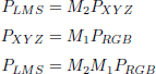
The algorithm that we present in this section makes it possible to insert a mark in a color image whose quality is improved from a psychovisual point of view. Compared to a classical insertion scenario, we suggest adding a step to adapt insertion to the color space (illustrated in Figure 4.7).
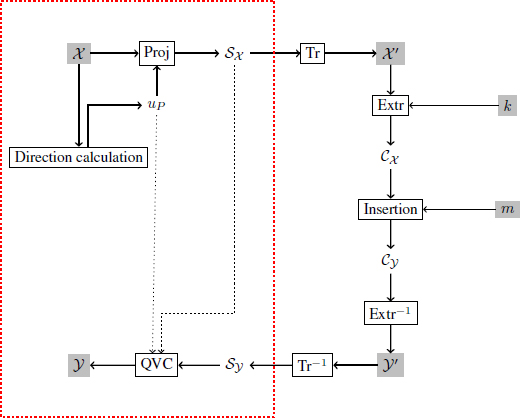
Figure 4.7. Classical insertion diagram combined with color vector quantization (QVC) based on a psychovisual model. The elements within the red frame represent the steps of vector quantization. Tr() and Extr() are the space transformation and coefficient extraction functions, k is the secret key and m is the binary message
Before transforming the host image in the chosen quantization space, we calculate a direction vector for each color pixel of the image χ. This direction vector will be defined from the optimal axis presented in section 4.4.6. Then we introduce the scalar product, s (the “Proj” step in Figure 4.7).
We then obtain a scalar value image ![]() . Considering the knowledge of the set of computed direction vectors, we have a one-to-one correspondence between χ and
. Considering the knowledge of the set of computed direction vectors, we have a one-to-one correspondence between χ and ![]() . In Figure 4.8, we can see that image
. In Figure 4.8, we can see that image ![]() is a dark grayscale version of the color image χ.
is a dark grayscale version of the color image χ.
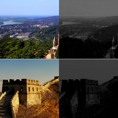
Figure 4.8. Pairs of images (host image χ, associated scalar image  ). Random images from the Corel database (available at: https://sites.google.com/site/dctresearch/Home/content-based-image-retrieval)
The next step then involves changing the representation of ![]() . A good first choice of representation is the spatial domain, but a transformed space can be used (transformed into discrete cosine [DCT] or transformed into wavelet coefficients [DWT]). These different representations (denoted Tr and Tr−1 for the inverse operation) of the image make it possible to obtain useful properties according to requirements, such as breaking the image down into independent frequency bands.
. A good first choice of representation is the spatial domain, but a transformed space can be used (transformed into discrete cosine [DCT] or transformed into wavelet coefficients [DWT]). These different representations (denoted Tr and Tr−1 for the inverse operation) of the image make it possible to obtain useful properties according to requirements, such as breaking the image down into independent frequency bands.
An extraction function Extr must then be chosen in order to select the coefficients to be changed. In this chapter, we have chosen a function which randomly determines insertion sites of the image ![]() . Another method for selecting coefficients was presented in Chapter 3, which involves breaking an image down into blocks and then randomly selecting coefficients in each block. The result of this extraction takes place in the watermarking space, which is a secret space (known only to the creator of the mark and its recipient). Access to this space can be secured with a secret key k.
. Another method for selecting coefficients was presented in Chapter 3, which involves breaking an image down into blocks and then randomly selecting coefficients in each block. The result of this extraction takes place in the watermarking space, which is a secret space (known only to the creator of the mark and its recipient). Access to this space can be secured with a secret key k.
Once the coefficients ![]() are selected, they are modified by the insertion method (the LQIM method, but it is also possible to use other watermarking methods) according to the message m, then integrated into the representation of the image used for extraction and we get the marked image
are selected, they are modified by the insertion method (the LQIM method, but it is also possible to use other watermarking methods) according to the message m, then integrated into the representation of the image used for extraction and we get the marked image ![]() ′. So, for any modified color P′ (QVC stage), we have:
′. So, for any modified color P′ (QVC stage), we have:
where s′ is the scalar modified by the chosen insertion method.
The set of s′ forms the grayscale image ![]() . Of course, note that the use of different error correcting codes, such as those proposed in Chapter 3 (e.g. Hamming, BCH, Reed–Solomon and Gabidulin codes), is completely possible and straightforward. In this chapter, we focus only on the “invisibility control” aspect and its optimization with respect to robustness.
. Of course, note that the use of different error correcting codes, such as those proposed in Chapter 3 (e.g. Hamming, BCH, Reed–Solomon and Gabidulin codes), is completely possible and straightforward. In this chapter, we focus only on the “invisibility control” aspect and its optimization with respect to robustness.
At the detection stage (Figure 4.9), we identify the grayscale image ![]() by recalculating the direction vectors associated with each color of the image received
by recalculating the direction vectors associated with each color of the image received ![]() (equation [4.23]), and then accessing the watermark channel using the Extr extraction function and the key k.
(equation [4.23]), and then accessing the watermark channel using the Extr extraction function and the key k.
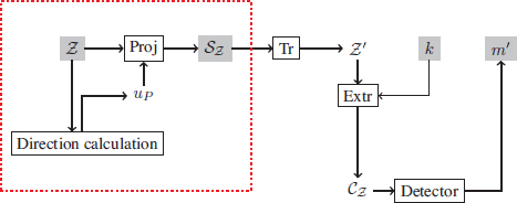
Figure 4.9. Classical mark detection diagram. As with insertion, we find the extraction part of the scalar image  framed in red
We then apply the detector associated with the chosen insertion method to the coefficients ![]() . If the power of the attack is reasonable and the mark robustness parameters are well chosen, the estimate m′ should be the same as m.
. If the power of the attack is reasonable and the mark robustness parameters are well chosen, the estimate m′ should be the same as m.
As we said for the detection, the calculation of the direction vectors is an important step. Assuming that the colors are reasonably modified, the ability to correctly detect the message lies in the variation of the direction vector. In our experiments we will see that the variations of the direction vectors are acceptable and make it possible to ensure good detection.
We have detailed a classical watermarking algorithm for color images using a color vector quantization method based on a psychovisual model of the HVS. The LQIM method was chosen to be adapted to watermarking color images (introduced in section 4.2). To be able to use it, we adapt the classical insertion diagram with our psychovisual quantization model 4.7, then we integrate the quantifier Qm into the insertion function of the LQIM method. The insertion sites are chosen randomly from the coefficients available for insertion. One of the advantages of this insertion strategy is improving the invisibility of the mark, especially in textured areas of the image. At the detection stage, we also combine the extraction stage of the received coefficients ![]() (Figure 4.9) with the classical decoding scheme using the LQIM detector.
(Figure 4.9) with the classical decoding scheme using the LQIM detector.
Section 4.4.8 gives an evaluation of the robustness performance of the CLQIM method against various image modifications.
4.4.8. Experimental validation of the psychovisual approach for color watermarking
The images used for the experiments belong to the Corel database (1,000 random images selected from the 10,000 available). The insertion sites are determined randomly. To evaluate the invisibility, parameters such as the size of the message or the dimension of the Euclidean lattice L of the Lattice QIM method are calculated in order to obtain an adequate image quality and an adequate insertion rate.
4.4.8.1. Validation of invisibility
In this section, we propose different groups of marked images in order to appreciate the improvement in invisibility, compared to marked images following a vector quantization of constant direction vector.
We then denote the following two approaches by GA and AA:
- – the color version with a constant direction axis u = (1, 1, 1) (GA). We have chosen this direction vector because choosing the luminance axis is, in our opinion, a satisfactory compromise in order to guarantee a good level of invisibility of a mark;
- – the color version with an adaptive direction axis uP (AA).
These two watermarking methods are the color adaptations of the LQIM method previously presented in this chapter. For each approach, the direction vectors are the same magnitude (arbitrarily set at 0.5). For the same level of digital distortion, it is a question of validating, through experimentation, that the AA approach inserts a less visible mark than the GA approach.
In these experiments, we evaluate the digital distortion thanks to the signal-to-noise ratio, characterizing the quantization noise of the LQIM method, denoted as DWR.
In Figure 4.10, we show examples of color images marked with the GA approach of the LQIM method. For each image in this figure, we can easily see that the colors saturate toward gray. It therefore becomes easier to perceive color differences by comparing them to neighboring pixels. The visual appearance of quantization noise is salt and pepper noise and it adds texture to the image.
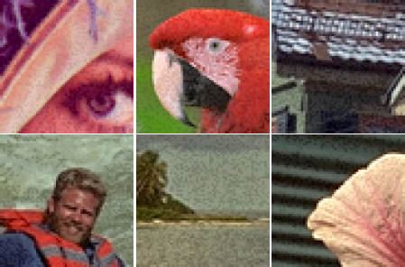
Figure 4.10. Cropped color images (Lena and Kodak base of size 60 × 60) marked with the LQIM method (GA approach), DWR ≃ − 5.5 dB on average and ER = 0.5
With the AA approach (Figure 4.11), the quantization noise has the effect of saturating the colors toward blue and green. This adapts according to the modified color. It is therefore more difficult to perceive the noise. Compared to neighboring pixels in areas of the same color, we find that detecting color difference is difficult.
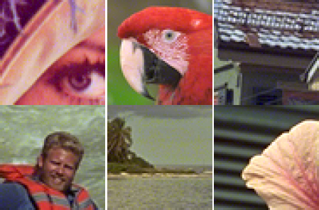
Figure 4.11. Cropped color images (Lena and Kodak base of size 60 × 60) marked with the LQIM method (AA approach), DWR ≃ 5.5 dB on average and ER = 0.5
At equal digital distortion, images marked with the GA and AA approaches are not affected with the same quantization noise from a psychovisual point of view. The perception of quantization noise with the AA approach is much lower for the HVS compared to that of the AA approach. We can see this in the images of Figures 4.10 and 4.11, but these results were also confirmed in other tests.
To able to better observe the insertion noise, we have chosen images of size 60 × 60 and have chosen a strong insertion rate (ER = 0.5). In practice, the images are much larger in size (e.g. 1,080 × 1,920 for high definition) and the insertion rate is weaker, which makes the insertion noise less visible for the HVS.
We repeated the comparison experiment of the GA and AA approaches described above with different observers (15 in number) and with the Kodak image base, composed of 24 elements of size 768 × 512. For each image of this database, we offered a pair of images marked with the two color approaches GA and AA (still with the LQIM method). For the 24 pairs of images, each observer voted for the “least noisy” image.
The results of this experiment are presented in Table 4.1. Of these subjects, only 4% of images on average were described as “least noisy” with the GA approach. Of these results, we conclude that the use of a psychovisual model allows us to obtain a much better invisibility.
Table 4.1. Psychovisual experiments of marked image comparisons
| Approaches | GA approaches | AA approaches |
|---|---|---|
| Average votes | 4 ± 3% | 96 ± 3% |
COMMENT ON TABLE 4.1.– Each person had to decide which of the images was more degraded (a watermarked image with the constant approach, and the other with the adaptive approach). The parameters are DWR = 20 dB, ER = 0.5 for each image. This table shows the percentage of images noted as less degraded for each approach.
We now intend to compare the two approaches in terms of their robustness performance against several image modifications. We offer a simple experiment for this. We propose to insert a message of size n = 128 bits. In order to ensure satisfactory image quality and mark invisibility, we determined the average maximum quantization step before a mark was visible for each method. We measured average bit error rates (100 repetitions for the same quantization step) depending on the strength of the applied image modification. We now propose to analyze the robustness against classical attacks.
4.4.8.2. Impact on robustness
4.4.8.2.1. Modification of luminance
We model the modification of luminance by equation [4.25]:
where y is the modified version of x, the value of a pixel.
The robustness results are shown in Figure 4.12. The error curves oscillate like a step function between 0 and 1 periodically. This attack is special because it applies modifications that are not dependent on the image. This behavior is justified, both by the use of the LQIM method, and by the structure of the error produced by the modification of luminance (studied in detail in Chapter 3).
For the LQIM AA curve, the oscillation period is greater than that of the LQIM GA curve, which gives a larger error-free interval around 0.
4.4.8.2.2. Modification in the HSV space
We now consider examples of color image modifications. By representing an image in the HSV color space, we modify each color component h, s and v.
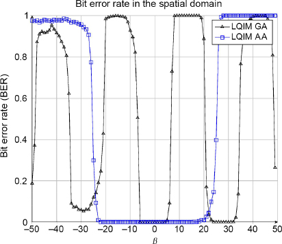
Figure 4.12. Binary error for methods GA and AA depending on the parameter β
In Figure 4.13(b), we observe that the LQIM AA SP curves are closer to 0 than the LQIM GA SP curves on each component, therefore showing that taking an HVS model into account allows us to improve the robustness of a watermarking algorithm, not just its invisibility.
4.5. Conclusion
In this chapter, we have dealt with the challenge of the invisibility of hidden information in the context of color images. For this, the latest developments of digital watermarking for color images have been proposed. We find that the majority of the methods are an extension of the approaches for grayscale images. We then showed that, in many cases, the key is wisely choosing the color direction vector at insertion, and this is true even with dedicated spaces, such as quaternions. We then recalled the impact of this direction choice and discussed the importance of taking the HVS into account.
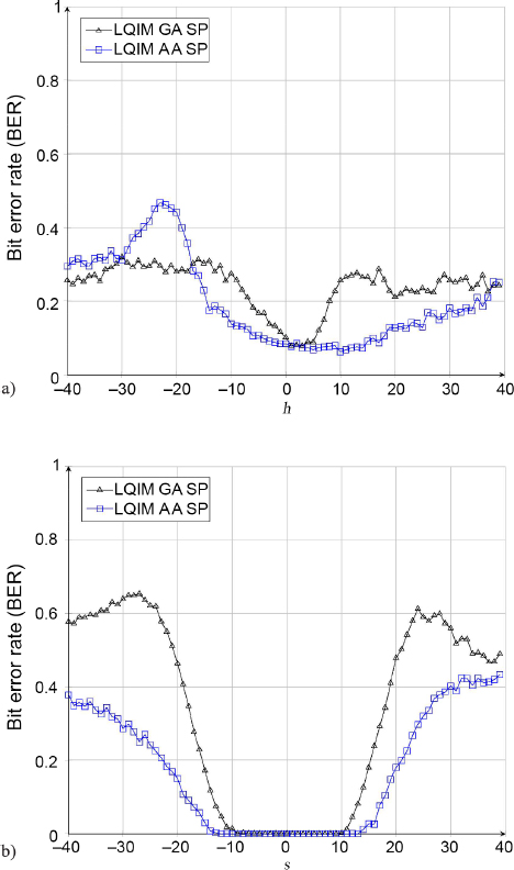
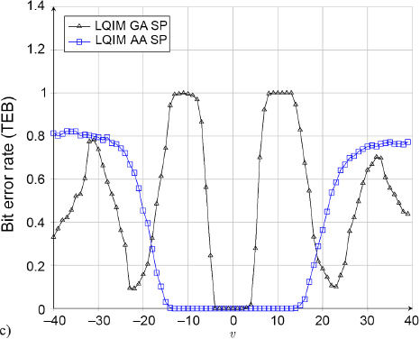
Figure 4.13. Bit error rate for (a) hue; (b) saturation; and (c) value modification
We then discussed a psychovisual approach, allowing us to model the behavior of photoreceptors in the human retina. Thanks to the calibration of the constants, based on the measurements of MacAdam ellipses, the photoreceptor model makes it possible to simulate the behavior of an average HVS in terms of the perception of color differences. We then applied it to digital watermarking of color images in order to extract the direction vectors needed for vector quantization and chose to adapt the LQIM method to make it able to watermark color images. In terms of invisibility, this method makes it possible to obtain much better invisibility than a non-adaptive method with equal digital distortion. We also see an improvement in robustness. The last section shows the importance of this parameter in an invisibility problem for color watermarking.
4.6. References
Abadpour, A. and Kasaei, S. (2008). Color PCA eigenimages and their application to compression and watermarking. Image and Vision Computing, 26(7), 878–890.
Alleysson, D. (1999). Le traitement du signal chromatique dans la rétine : un modèle de base pour la perception humaine des couleurs. PhD Thesis, Joseph Fourier University, Grenoble.
Alleysson, D. and Hérault, J. (2001). Variability in color discrimination data explained by a generic model with nonlinear and adaptive processing. Color Research & Application, 26(S1), S225–S229.
Alleysson, D. and Méary, D. (2012). Neurogeometry of color vision. Journal of Physiology – Paris, 106(5–6), 284–296.
Assefa, D., Mansinha, L., Tiampo, K.F., Rasmussen, H., Abdella, K. (2010). Local quaternion Fourier transform and color image texture analysis. Signal Processing, 90(6), 1825–1835.
Bas, P., Le Bihan, N., Chassery, J.-M. (2003). Color image watermarking using quaternion Fourier transform. In International Conference on Acoustics, Speech, and Signal Processing, Hong Kong, 6–10 April.
Carré, P., Denis, P., Fernandez-Maloigne, C. (2012). Spatial color image processing using Clifford algebras: Application to color active contour. Signal, Image and Video Processing, 8(7), 1357–1372.
Chareyron, G. and Trémeau, A. (2006). Color images watermarking based on minimization of color differences. In International Workshop on Multimedia Content, Representation, Classification and Security, Istanbul, Turkey, 11–13 September.
Chareyron, G., Macq, B., Tremeau, A. (2004). Watermarking of color images based on segmentation of the XYZ color space. In Conference on Colour in Graphics, Imaging, and Vision, 1, 178–182 Aachen, Germany, 5–8 April.
Chou, C. and Liu, K. (2010). A perceptually tuned watermarking scheme for color images. IEEE Transactions on Image Processing, 19(11), 2966–2982.
Coltuc, D. and Bolon, P. (1999). Robust watermarking by histogram specification. In International Conference on Image Processing, 2, 236–239, Kobe, Japan, 24–28 October.
Dadkhah, S., Manaf, A.A., Hori, Y., Hassanien, A.E., Sadeghi, S. (2014). An effective SVD-based image tampering detection and self-recovery using active watermarking. Signal Processing: Image Communication, 29(10), 1197–1210.
Denis, P., Carre, P., Fernandez-Maloigne, C. (2007). Spatial and spectral quaternionic approaches for colour images. Computer Vision and Image Understanding, 107(1), 74–87.
Ell, T.A. and Sangwine, S.J. (2000). Decomposition of 2D hypercomplex Fourier transforms into pairs of complex Fourier transforms. In 10th European Signal Processing Conference, 1–4, Tampere, Finland, 4–8 September.
Ell, T.A. and Sangwine, S.J. (2006). Hypercomplex Fourier transforms of color images. IEEE Transactions on Image Processing, 1(16), 22–35.
Hu, R., Chen, F., Yu, H. (2010). Incorporating Watson’s perceptual model into patchwork watermarking for digital images. In International Conference on Image Processing, 3705–3708, Hong Kong, 26–29 September.
Kim, H.-S., Lee, H.-K., Lee, H.-Y., Ha, Y.-H. (2001). Digital watermarking based on color differences. Security and Watermarking of Multimedia Contents III, 4314, 10–17.
Koenderink, J., van de Grind, W., Bouman, M. (1970). Models of retinal signal processing at high luminances. Kybernetik, 6(6), 227–237.
Kutter, M., Jordan, F.D., Bossen, F. (1997). Digital signature of color images using amplitude modulation. SPIE, 3022, 518–526.
Li, Q. and Cox, I.J. (2007). Using perceptual models to improve fidelity and provide resistance to valumetric scaling for quantization index modulation watermarking. IEEE Transactions on Information Forensics and Security, 2(2), 127–139.
Li, J., Lin, Q., Yu, C., Ren, X., Li, P. (2018). A QDCT- and SVD-based color image watermarking scheme using an optimized encrypted binary computer-generated hologram. Soft Computing, 22, 47–65.
MacAdam, D.L. (1942). Visual sensitivities to color differences in daylight. Josa, 32(5), 247–274.
Parisis, A., Carre, P., Fernandez-Maloigne, C., Laurent, N. (2004). Color image watermarking with adaptive strength of insertion. In International Conference on Acoustics, Speech, and Signal Processing, 81–85, Montreal, Canada, 17–21 May.
Petitot, J. (2003). The neurogeometry of pinwheels as a sub-Riemannian contact structure. Journal of Physiology – Paris, 97(2), 265–309.
Petitot, J. (2008). Neurogéométrie de la vision : modèles mathématiques et physiques des architectures fonctionnelles. Éditions de l’École Polytechnique, Palaiseau.
Sangwine, S. (2000). Colour in image processing. Electronics and Communication Engineering Journal, 12(5), 211–219.
Sangwine, S. and Ell, T. (2001). Hypercomplex Fourier transforms of color images. In International Conference on Image Processing, 137–140, Thessaloniki, Greece, 7–10 October.
Tsui, T.K., Zhang, X., Androutsos, D. (2008). Color image watermarking using multidimensional Fourier transforms. IEEE Transactions on Information Forensics and Security, 3(1), 16–28.
Voyatzis, G. and Pitas, I. (1998). Digital image watermarking using mixing systems. Computers & Graphics, 22, 405–416.
Wan, W., Zhou, K., Zhang, K., Zhan, Y., Li, J. (2020). JND-guided perceptually color image watermarking in spatial domain. In IEEE Access, 8, 164504–164520.
Watson, A.B. (1993). DCT quantization matrices visually optimized for individual images. In IS&T/SPIE’s Symposium on Electronic Imaging: Science and Technology, San Jose, 31 January–5 February.
Yu, P.-T., Tsai, H.-H., Lin, J.-S. (2001). Digital watermarking based on neural networks for color images. Signal Processing, 81(3), 663–671.
Zrenner, E., Stett, A., Weiss, S., Aramant, R.B., Guenther, E., Kohler, K., Miliczek, K.-D., Seiler, M.J., Haemmerle, H. (1999). Can subretinal microphotodiodes successfully replace degenerated photoreceptors? Vision Research, 39(15), 2555–2567.
- For a color version of all figures in this chapter, see www.iste.co.uk/puech/multimedia1.zip.
- 1 White point of equal energy E.