
Space Odyssey – Stereo and spatial sound
Stereo
When listening to music on a two-channel stereo audio system, a sound ‘image’ is spread out in the space between the two loudspeakers. The reproduced image thus has some characteristics in common with the way the same music is heard in real life – that is, with individual instruments or voices each occupying, to a greater or lesser extent, a particular and distinct position in space. Insofar as this process is concerned with creating and re-creating a ‘sound event’, it is woefully inadequate. First, the image is flat and occupies only the space bounded by the loudspeakers. Second, even this limited image is distorted with respect to frequency. (There exists an analogy with chromatic aberration in optics.) Happily there exist relatively simple techniques for both the improvement of existing stereophonic images and for the creation of synthetic sound fields in a 360° circle around the listening position. The basic techniques of stereophony and these newer techniques, are covered later on in this chapter, but first there is a brief review of spatial hearing – our capacity to localise (determine the position of) a sound in our environment.
Spatial hearing
Sound localisation in humans is remarkably acute. As well as being able to judge the direction of sounds within a few degrees, experimental subjects are sometimes able to estimate the distance of a sound source as well. Consider the situation shown in Figure 11.1, where an experimental subject is presented with a source of steady sound located at some distance from the side of the head. The two most important cues the brain uses to determine the direction of a sound are due to the physical nature of sound and its propagation through the atmosphere and around solid objects. We can make two reliable observations:

1. at high frequencies, the relative loudness of a sound at the two ears is different since the nearer ear receives a louder signal compared with the remote ear; and
2. at all frequencies, there is a delay between the sound reaching the near ear and the further ear.
It can be demonstrated that both effects aid the nervous system in its judgement as to the location of a sound source: at high frequencies, the head casts an effective acoustic ‘shadow’ which acts like a low-pass filter and attenuates high frequencies arriving at the far ear, thus enabling the nervous system to make use of interaural intensity differences to determine direction. At low frequencies, sound diffracts and bends around the head to reach the far ear virtually unimpeded. So, in the absence of intensity-type directional cues, the nervous system compares the relative delay of the signals at each ear. This effect is termed interaural delay difference. In the case of steady-state sounds or pure tones, the low-frequency delay manifests itself as a phase difference between the signals arriving at either ear. The idea that sound localisation is based upon interaural time differences at low frequencies and interaural intensity differences at high frequencies has been called Duplex theory and it originates with Lord Rayleigh at the turn of the century.1
Binaural techniques
In 1881, Monsieur Clement Ader placed two microphones about eight inches apart (the average distance between the ears known technically as the interaural spacing) on stage at the Paris Opera where a concert was being performed and relayed these signals over telephone lines to two telephone earpieces at the Paris Exhibition of Electricity. The amazed listeners were able to hear, by holding one earpiece to each ear, a remarkably lifelike impression that they too were sitting in the Paris Opera audience. This was the first public demonstration of binaural stereophony, the word binaural being derived from the Latin for two ears.
The techniques of binaural stereophony, little different from this original, have been exploited many times in the century since the first demonstration. However, psychophysicists and audiologists have gradually realised that considerable improvements can be made to the simple spaced microphone system by encapsulating the two microphones in a synthetic head and torso. The illusion is strengthened still more if the dummy head is provided with artificial auricles (external ears or pinnae – see Chapter 2). The binaural stereophonic illusion is improved by the addition of an artificial head and torso and external ears because it is now known that sound interacts with these structures before entering the ear canal. If, in a recording, microphones can be arranged to interact with similar features, the illusion is greatly improved in terms of realism and accuracy when the signals are relayed over headphones. This is because headphones sit right over the ears and thus do not interact with the listener’s anatomy on the final playback.
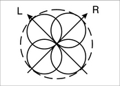
The most significant effect brought about by the addition of artificial auricles is the tendency for the spectrally modified sound events to localise outside of the listener’s head as they do in real life. Without these additions the sound image tends to lateralise – or remain artificially inside the head. And they play another role: we saw in Figure 11.1 that the main cues for spatial hearing lay in the different amplitudes and phases of the signals at either ear. Such a system clearly breaks down in its ability to distinguish from a sound directly in front from one directly behind (because, in both cases, there are neither amplitude nor phase differences in the sounds at the ears – see Figure 11.2). A little thought reveals that the same thing goes for a sound from any direction – it is always possible to confuse a sound in the forward 180° arc from its mirror image in the rear 180° arc. A common failing of binaural stereophonic recordings (made without false pinnae) is the erroneous impression, gained on playback, that the recorded sound took place behind the head, rather than in front. Manifestly, the pinnae appear to be involved in reducing this false impression and there exist a number of excellent experimental papers describing this role, known as investigations into the front–back impression (Blauert 1983).

Two-loudspeaker stereophony
If the signals from a dummy head recording are replayed over two loudspeakers placed in the conventional stereophonic listening arrangement (as shown in Figure 11.3), the results are very disappointing. The reason for this is the two unwanted crosstalk signals: The signal emanating from the right loudspeaker which reaches the left ear; and the signal emanating from the left loudspeaker which reaches the right ear (shown in Figure 11.4). These signals result in a failure to reproduce the correct interaural time delay cues at low frequencies. Furthermore, the filtering effects of the pinnae (so vital in obtaining out-of-the-head localisation when listening over headphones) are not only superfluous, but impart to the sound an unpleasant and unnatural tonal balance. Because of these limitations binaural recordings are made only in special circumstances. A different technique is used in the production of most stereo records and CDs. A system was invented in 1928 by Alan Blumlein – an unsung British genius. Unfortunately Blumlein’s solution is so complete – and so elegant – that it is still widely misunderstood or regarded as simplistic.


Summing localisation
Consider the arrangement shown in Figure 11.3 again. A moment’s thought will probably lead you to some fairly obvious conclusions: if all the sound comes out of the left loudspeaker, the listener will clearly experience the sound ‘from the left’. Similarly with the right. If both loudspeakers reproduce identical sounds at identical intensity, it is reasonable to assume that the listener’s brain will conclude the existence of a ‘phantom’ sound, coming from directly in front, because in nature that situation will result in the sound at both ears being identical. And indeed it does, as experiments have confirmed. Furthermore proportionally varied signal intensities result in a continuum of perceived ‘phantom’ image positions between the loudspeakers. But how does a system which works on intensity alone fool the brain into thinking there is a phantom sound source other than in the three rather special positions noted above? While it is fairly obvious that interchannel intensity differences will reliably result in the appropriate interaural intensity differences at high frequencies, what about at low frequencies where the sound can diffract around the head and reach the other ear? Where does the necessary low-frequency time-delay component come from?
When two spaced loudspeakers produce identically phased low-frequency sounds at different intensities, the soundwaves from both loudspeakers travel the different distances to both ears and arrive at either ear at different times. Figure 11.5 illustrates the principle involved: the louder signal travels the shorter distance to the right ear and the longer distance to the left ear. But the quieter signal travels the shorter distance to the left ear and the longer distance to the right ear. The result is that the sounds add vectorially to the same intensity but different phase at each ear. The brain interprets this phase information in terms of interaural delay. Remember that stereophonic reproduction from loudspeakers requires only that stereo information be carried by interchannel intensity difference. Despite a huge body of confused literature to the contrary, there is no requirement to encode interchannel delay difference. If this were not the case, the pan control, which the sound engineer uses to ‘steer’ instruments into position in the stereo ‘sound stage’, would not be the simple potentiometer control described in the next chapter.

FRANCINSTIEN stereophonic image enhancement technique
So far we have only considered individual sounds; however, stereo works by eliciting, within the mind of the listener, a continuum of simultaneous and coexistent stereo images for each voice and/or instrument. As we have seen, at high frequencies, the stereo image is largely intensity derived and, at low frequency the image is largely delay derived. Unfortunately, conventional intensity-derived two loudspeaker stereo cannot create a perfect illusion, the problem being that the simultaneous stereo images (one set predominantly high frequency and the other predominantly low frequency) are not in exact perceptual spatial register. In this section, circuitry is described which electrically manipulates the signals of an existing stereophonic recording, to bring about an improvement in the realism of two-speaker stereophonic reproduction. A review of the literature reveals that the technique is not new. Nevertheless the implementation described is both radical and novel and side-steps many of the problems and awkwardness of the previous attempts to solve this frequency dependent ‘smearing’ of the stereo image described here.
The important qualitative fact to appreciate is that, for a given interchannel intensity difference, the direction of the perceived auditory event is further from a central point between the loudspeakers when a high-frequency signal is reproduced than when a low frequency is reproduced. Since music is itself a wideband signal, when two loudspeakers reproduce a stereo image from an interchannel intensity derived stereo music signal, the high-frequency components of each instrument or voice will subtend a greater angle than will the low-frequency components. This problem was appreciated even in the very early days of research on interchannel intensity related stereophony and, through the years, a number of different solutions have been proposed.
The Shuffler
Blumlein mentioned in his 1931 patent application that it was possible to control the width of a stereo image by matrixing the left and right signal channels into a sum and difference signal pair and controlling the gain of the difference channel prior to rematrixing back to the normal left and right signals. He further suggested that, should it be necessary to alter the stereo image width in a frequency dependent fashion, all that was needed was a filter with the appropriate characteristics to be inserted in this difference channel. After his untimely death, the post-war team working at EMI on a practical stereo system and attempting to cure this frequency dependent ‘smearing’ of the stereo picture implemented just such an arrangement and introduced a filter of the form:
into the difference channel. Figure 11.6 is an illustration of their practical Shuffler circuit (as they termed it) and its implementation in the difference channel. Unfortunately this circuit was found to introduce distortion and tonal colouring and was eventually abandoned. (It has been demonstrated that the time constants and attenuation ratios used in the original Shuffler circuit were not, in any case, well chosen.) Nevertheless it is well worth investigating the Shuffler technique because it demonstrates particularly clearly the requirement for any mechanism designed to tackle the image blurring problem.
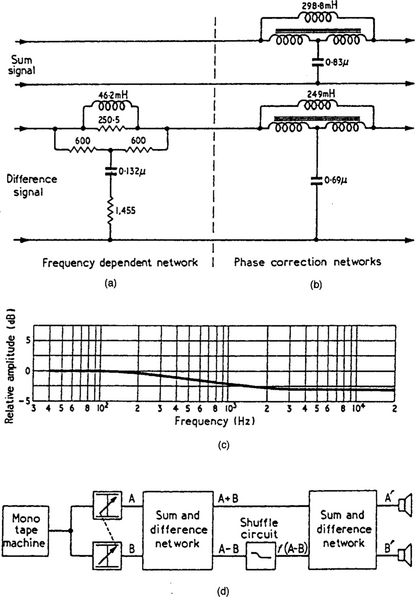
Manifestly, there is only one particular filter characteristic which will equalise the interchannel intensity difference signal in the appropriate fashion. If we rewrite the above equation, the characteristics for such a filter become easier to conceptualise:
This is because the variable A represents overall difference-channel gain, and demonstrates how overall image width may be manipulated, and further, since
the term a1/a2 defines the image narrowing at high frequency and demonstrates the filtering necessary to match the interaural intensity derived high-frequency image with the interaural delay derived image at low frequency. One might therefore call a1 and a2, psychoacoustic constants. It was precisely these constants which were at fault in the original Shuffler circuit.
Other derivatives of the Shuffler, using operational amplifier techniques, have appeared, but the act of matrixing, filtering and rematrixing is fraught with problems since it is necessary to introduce compensating delays in the sum channel which very exactly match the frequency dependent delay caused by the filters in the difference channel if comb filter coloration effects are to be avoided. Furthermore the very precise choice of the correct constants is crucial. After all, existing two-loudspeaker stereo is generally regarded as being a tolerably good system, the required signal manipulation is slight and failure to use the correct constants, far from improving stereo image sharpness, can actually make the frequency dependent blurring worse! Others have taken a more imaginative and unusual approach.
Edeko
It is a fundamental characteristic of the blurring problem that the brain perceives the high-frequency intensity derived image as generally wider than the low-frequency, delay derived image. With this in mind Dr Edeko conceived of a way of solving the problem acoustically (and therefore of side-stepping the problems which beset electronic solutions).
Edeko (1988) suggested a specially designed loudspeaker arrangement as shown in Figure 11.7 where the angle between the high frequency loudspeaker drive units subtended a smaller angle at the listening position than the mid-range drive units and these, in turn, subtended a smaller angle than the low-frequency units. This device, coupled with precise designs of electrical crossover network enabled the image width to be manipulated with respect to frequency.

Improving image sharpness by means of interchannel crosstalk
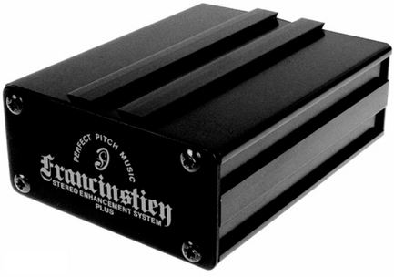
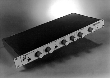
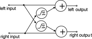
There is a much simpler technique which may be used to narrow a stereo image at high frequencies and that is by the application of periodic interchannel crosstalk (Brice 1997). Interestingly investigations reveal that distortion mechanisms in reproduction from vinyl and other analogue media may indeed be just those required to bring about an improvement in the realism of the reproduced stereo image.2 This suggests there may be something in the hi-fi cognoscenti’s preference for vinyl over CD and for many recording musicians’ preference for analogue recording over the, apparently better, digital alternative – though not, as they invariably suppose, due to digital mysteriously taking something away but due to the analogue equipment adding beneficial distortion. This crosstalk technique is exploited in the FRANCINSTIEN range of stereophonic image enhancement systems developed by Perfect Pitch Music Ltd. Commercial units for use in hi-fi systems and recording studios are illustrated in Figures 11.8 and 11.9. The simplest possible implementation of the FRANCINSTIEN effect is achieved very easily. The schematic is given in Figure 11.10. This circuit may be included in the record or replay chain but not both.
3D sound fields
Perhaps the crudest method for generating audible spatial effects is to provide more channels of audio and more loudspeakers!
Dolby Surround
Walt Disney Studio’s Fantasia was the first film ever to be shown with a stereo soundtrack. That was in 1941. Stereo in the home has been a reality since the 1950s. Half a century on, it is reasonable that people might be looking for ‘something more’. With the advent of videocassette players, watching film at home has become a way of life. Dolby Surround was originally developed as a method of bringing part of the cinema experience to the home where a similar system named Dolby Stereo has been in use since 1976. Like Dolby Stereo, Dolby Surround is essentially a four-channel audio system encoded or matrixed into the standard two-stereo channels. Because these four discrete channels are encoded within the stereo channels extra hardware is required both at the production house and in the home. Decoders are now very widespread because of the take-up of home cinema systems. The extra hardware required, in addition to normal stereo, is a number of extra loudspeakers (ideally three), a decoder and an extra stereo power amplifier. Some manufacturers supply decoder and four power amplifiers in one AV amplifier unit. In addition a sub-woofer channel may be added. (A sub-woofer is a loudspeaker unit devoted to handling nothing but the very lowest audio frequencies – say below 100 Hz.) Frequencies in this range do add a disproportionate level of realism to reproduced sound. In view of the very small amount of information (bandwidth) this is surprising. However, it is likely humans infer the scale of an acoustic environment from these subsonic cues. (Think about the low, thunderous sound of the interior of a cathedral.)
In order for an audio, multimedia or VR studio to produce Dolby Surround material, and claim that it is such, permission has to be granted by Dolby who provide the encoding unit and a consultant on a daily basis. (You have, of course, also to set up your studio so that it has the necessary decoding facilities by buying extra loudspeakers, decoder and amplifiers.) This is fine if you’re a Hollywood film company but less good if you’re an independent producer of video, audio or multimedia material. Fortunately, while you will not be able to mark your studio productions as Dolby Surround encoded there is no reason why you may not encode information so that you can exploit the effects of Dolby Surround decoding. In fact encoding is much simpler than decoding and this is discussed in this section. But first a description of the Dolby Surround process.
A typical surround listening set-up is illustrated in Figure 11.11. Note the extra two channels, centre and surround, and the terminology for the final matrixed two channels signals Lt and Rt; standing for left-total and right-total respectively. The simplest form of decoder (which most certainly does not conform to Dolby’s criteria but is nevertheless reasonably effective) is to feed the centre channel power amplifier with a sum signal (Lt + Rt) and the surround channel amplifier with a difference signal (Lt – Rt). This bare-bones decoder works because it complements (to a first approximation) the way a Dolby Surround encoder matrixes the four channels onto the left and right channel: centre channel split between left and right, surround channel split between left and right with one channel phase reversed. If we label the original left/right signals L and R we can state the fundamental process formally:
| Input channels | |
| Left (sometimes called left music channel): | L |
| Right (sometimes called right music channel): | R |
| Centre channel (sometimes called dialogue channel): | C |
| Surround channel (for carrying atmosphere sound effects etc.). | S |
Output channels (encoding process)

where i, j and k are simply constants. And the decoding process yields:
| Left (L’) | = e(Lt) | |
| Right (R’) | = f(Rt) | |
| Centre (C’) | = u(Lt + Rt) | = u[i(L + jC + kS + R + jC – kS)] |
| = u[i(L + R + 2jC)] | ||
| Surround (S’) | = v(Lt – Rt) | = v[i(L + jC + kS – R – jC + kS)] |
| = v[i(L – R + 2kS)] |
where e and f and u and v are constants.
Which demonstrates this is far from a perfect encoding and decoding process. However a number of important requirements are fulfilled even by this most simple of matrixing systems and to some extent the failure mechanisms are masked by operational standards of film production. Dolby have cleverly modified this basic system to ameliorate the perceptible disturbance of these unwanted crosstalk signals. Looking at the system as a whole – as an encode and decode process, first, and most important, note that no original centre channel (C) appears in the decoded rear, surround signal (S’). Also note that no original surround signal (S) appears in the decoded centre channel (C’). This requirement is important because of the way these channels are used in movie production. The centre channel (C) is always reserved for mono dialogue. This may strike you as unusual but it is absolutely standard in cinema audio production. Left (L) and Right (R) channels usually carry music score. Surround (S) carries sound effects and ambience. Therefore, considering the crosstalk artefacts, at least no dialogue will appear in the rear channel – an effect which would be most odd! Similarly, although centre channel information (C) crosstalks into left and right speaker channels (L’ and R’), this only serves to reinforce the centre dialogue channel. The most troublesome crosstalk artefact is the v(iL – iR) term in the S’ signal which is the part of the left/right music mix which feeds into the decoded surround channel – especially if the mix contains widely panned material (with a high interchannel intensity ratio). Something really has to be done about this artefact for the system to work adequately and this is the most important modification to the simple matrix process stated above which is implemented inside all Dolby Surround decoders. All decoders delay the S’ signal by around 20 ms which, due to an effect known as the law of the first wavefront or the Hass effect, ensures that the ear and brain tend to ignore the directional information contained within signals which correlate strongly with signals received from another direction but at an earlier time. This is certainly an evolutionary adaptation to avoid directional confusion in reverberant conditions and biases the listener, in these circumstances, to ignore unwanted crosstalk artefacts. This advantage is further enhanced by band limiting the surround channel to around 7 kHz and using a small degree of high-frequency expansion (as explained in Chapter 6). Dolby Pro Logic enhances the system still more by controlling the constants written e, f, u and v above dynamically, based on programme information. This technique is known as adaptive matrixing.
One very important point to remember regarding Dolby Surround is that it does not succeed in presenting images at positions around the listening position. Instead the surround channel is devoted to providing a diffuse sound atmosphere or ambience. While this is effective, the system is not concerned with the creation of realistic (virtual) sound fields. Nevertheless, Dolby Surround systems with ProLogic are becoming a widespread feature in domestic listening environments and the wise musician-engineer could do worse than to exploit the emotive power this technology most certainly possesses. But how?
DIY surround mixing
Our understanding of Dolby replay has made it clear that encoding (for subsequent decoding by Dolby Surround decoders) can be undertaken quite simply. The golden rule, of course, is to set up a good surround monitoring system in the studio in the first place. Systems are available quite cheaply. With the monitoring system in place and adjusted to sound good with known material mixes can be undertaken quite simply: pan music mixes as normal – but avoid extreme pan positions. Ensure all narration (if appropriate) is panned absolutely dead centre. Introduce surround effects as mono signals fed to two channels panned hard left and right. Invert the phase of one of these channels. (Sometimes this is as simple as switching the channel phase invert button – if your mixer has one of these.) If it hasn’t you will have to devise a simple inverting operational amplifier stage with a gain of one. Equalise the ‘rear’ channels to roll off around 7 kHz, but you can add a touch of boost around 5 kHz to keep the sound crisp despite the action of the high-frequency expansion undertaken by the decoder.
Ambisonics
When mono recording was the norm, the recording engineer’s ideal was expressed in terms of the recording chain providing an acoustic ‘window’ at the position of the reproducing loudspeaker, through which the listener could hear the original acoustic event – a ‘hole in the concert hall wall’ if you like (Malham 1995). It is still quite common to see explanations of stereo which regard it as an extension of this earlier theory, in that it provides two holes in the concert wall! In fact such a formalisation (known as wavefront-reconstruction theory) is quite inappropriate unless a very great number of separate channels are employed. As a result, two-channel loudspeaker stereophony based on this technique – two wide-spaced microphones feeding two equally spaced loudspeakers – produces a very inaccurate stereo image. As we have seen, Blumlein took the view that what was really required was the ‘capturing’ of all the sound information at a single point and the recreation of this local sound field at the final destination – the point where the listener is sitting. He demonstrated that for this to happen, it required that the signals collected by the microphones and emitted by the loudspeakers would be of a different form to those we might expect at the listener’s ears, because we have to allow for the effects of crosstalk. Blumlein considered the recreation of height information (periphony) but he did not consider the recreation of phantom sound sources over a full 360° azimuth (pantophony). The recording techniques of commercial quad-raphonic3 systems (which blossomed in the 1970s) were largely based on a groundless extension of the already flawed wavefront-reconstruction stereo techniques and hence derived left-front, left-back signals and so on. Not so Ambisonics – brainchild of Michael Gerzon which although too a child of the 1970s and, in principle, a four-channel system, builds upon Blumlein’s work to create a complete system for the acquisition, synthesis and reproduction of enveloping sound fields from a limited number of loudspeakers.
Consider a sound field disturbed by a single sound source. The sound is propagated as a longitudinal wave which gives rise to a particle motion along a particular axis drawn about a pressure microphone placed in that sound field. Such a microphone will respond by generating an output voltage which is proportional to the intensity of the sound, irrespective of the direction of the sound source. Such a microphone is called omnidirectional because it cannot distinguish the direction of a sound source. If the pressure microphone is replaced with a velocity microphone, which responds to the particle motion and is therefore capable of being directional, the output is proportional to the intensity of the sound multiplied by cos I, where I is the angle between the angle of the incident sound and the major axis of the microphone response.
But there is an ambiguity as to the sound source’s direction if the intensity of the signal emerging from a velocity microphone is considered alone. As I varies from 0° to 359°, the same pattern of sensitivity is repeated twice over. On a practical level this means the microphone is equally responsive in two symmetrical lobes, known as the figure-of-eight response that we saw in Chapter 3. Mathematically put, this is because the magnitude of the each half-cycle of the cosine function is identical. But not in sign; the cosine function is negative in the second and third quadrant. So, this extra directional information is not lost, but is encoded differently, in phase information rather than intensity information. What is needed to resolve this ambiguity is a measure of reference phase to which the output of the velocity microphone can be compared. Just such a reference would be provided by a pressure microphone occupying a position, ideally coincident but practically very close to, the velocity type. (This explanation is a rigorous version of the qualitative illustration, in Figure 3.1, of the combination of a figure-of-eight microphone and an omnidirectional microphone ‘adding together’ to make a unidirectional, cardioid directional response.)
More intuitively stated: a velocity microphone sited in a sound field will resolve sound waves along (for instance) a left–right axis but not be able to resolve a sound from the left differently from a sound from the right. The addition of a pressure microphone would enable the latter distinction to be made by either subtracting or adding the signals from one another. Now consider rotating the velocity microphone so that it faced frontback. This time it would resolve particle motion along this new axis but would be equally responsive regardless of whether the sound came from in front or behind. The same pressure microphone would resolve the Situation. Now contemplate rotating the microphone again, this time so it faced up-down, the same ambiguity would arise and would once more be resolved by the suitable addition or subtraction of the pressure microphone signal.
Consider placing three velocity microphones each at right angles to one another (orthogonally) and, as nearly as possible in the same position in space. The combination of signals from these three microphones, coupled with the response of a single omnidirectional, phase-reference microphone, would permit the resolution of a sound from any direction. Which is the same thing as saying, that a sound in a unique position in space will translate to a unique combination of outputs from the four microphones. These four signals (from the three orthogonal velocity microphones and the single pressure microphone) are the four signals which travel in the four primary channels of an Ambisonics recording. In practical implementations, the up-down component is often ignored, reducing the system to three primary channels. These three signals may be combined in the form of a two-channel, compatible stereo signal in a process called UHJ coding, although this process is lossy. Ambisonics provides for several different loudspeaker layouts for reproduction.
If we consider the de facto four-speaker arrangement and limit the consideration of Ambisonics recording to horizontal plane only (three-channel Ambisonics), it is possible to consider rotating the velocity microphones so that, instead of facing front–back, left–right as described above, they face as shown in Figure 11.12. An arrangement which is identical to a ‘Blumlein’ crossed pair.
If we label one microphone L, the other R, and the third pressure microphone P as shown, by a process of simple addition and subtraction, four signals are obtainable from the combination of these three microphones:
each one equivalent to a cardioid microphone facing diagonally left-front, diagonally left-back, right front and right rear, in other words into the four cardinal positions occupied by the loudspeakers on replay. This approach is equivalent to the BBC’s policy on quadraphonic recording (Nisbett 1979). Ambisonics theory has enabled the construction of special Ambisonics panpots which enable sounds to be artificially positioned anywhere in a 360° sound stage based on simple channel intensity ratios.
Roland RSS system and Thorn EMI’s Sensaura
Anyone who has listened to a good binaural recording on headphones will know what an amazing experience it is, far more realistic than anything experienced using conventional stereo on loudspeakers. As noted earlier binaural recordings ‘fail’ on loudspeakers due to the crosstalk signals illustrated in Figure 11.4. A modern solution to this difficulty, known as crosstalk cancellation, was originally proposed by Schroeder and Atal (Begault 1994). The technique involves the addition, to the right-hand loudspeaker signal, of an out-of-phase version of the left channel signal anticipated to reach the right ear via crosstalk, and the addition, to the left-hand loudspeaker signal, of an out-of-phase version of the right-hand channel signal expected to reach the left ear via crosstalk. The idea is that these extra out-of-phase signals cancel the unwanted crosstalk signals, resulting in the equivalent of the original binaural signals only reaching their appropriate ears. Unfortunately, without fixing the head in a very precise location relative to the loudspeakers, this technique is very difficult to put into practice (Blauert 1985; Begault 1994) although several commercial examples exist, including the Roland RSS System and Thorn EMI’s Sensaura.
The Roland Corporation’s RSS system (Roland Sound Space) was introduced around 1990 and was primarily targeted at the commercial music industry. The original system consisted of a desktop control unit and a rack mount processor. The RSS system, illustrated in Figure 11.13, allowed up to four mono signals to be panned in 360° azimuth and elevation using the eight controls on the control unit. In essence the unit implemented a two-stage process. The first stage consisted of the generation of synthetic binaural signals followed by a second stage of binaural crosstalk cancellation. The unit also provided MIDI input so that the sound sources could be controlled remotely. Roland utilised a derivative of this technology in various reverb units (see Figure 11.14).
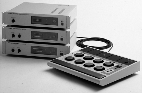
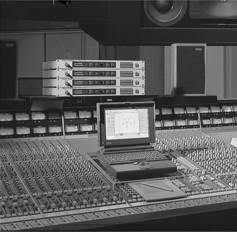
Figure 11.14 A later development of the unit shown in Figure 11.13
Thorn EMI’s Sensaura system also implemented a binaural crosstalk cancellation system, this time on signals recorded from a dummy head. There exists a paucity of technical information concerning this implementation and how it differs from that originally proposed by Schroeder and Atal (Begault 1994).
OM 3D sound processor
The RSS System and the Sensaura are intriguing systems because they offer the possibility of sound from all directions (pantophony) without the use of extra loudspeakers. The OM 3D sound system, developed by Perfect Pitch Music Ltd in Farnham, England, was developed with a similar goal in mind. The approach to the generation of two loudspeaker ‘surround sound’ taken in the OM system was an extension of summing stereophony. The OM system provided four mono inputs, two of which could be panned in a 180° arc which extended beyond the conventional loudspeaker boundary. Two further channels were provided which permitted sound sources to be panned 300°; from loudspeaker to loudspeaker in an arc to the rear of the stereo listening position. Figure 11.15 illustrates the two panning regimes. The unit was ideally integrated in a mixer system with four auxiliary sends. The resulting 3D-panned signals were summed on a common bus and output as a single stereo pair; the idea being that the output signal could be routed back to the mixer as a single stereo return. No provision was provided for adjusting the input sensitivity of any of the four input channels but VU meters allowed these levels to be monitored so that they could be set in the mixer send circuitry. Figure 11.16 is an illustration of the OM hardware and Figure 11.17 is a system diagram. Figure 11.18 illustrates the system configuration for a 3D mix. Looking first at channels 1 and 2; how was the 180° frontal pan achieved? OM was developed using a spatial hearing theory based upon Duplex theory. This approach suggests that any extension of the generation of spatial sound is best broken down in terms of high and low frequencies. Let’s take the low frequencies first.


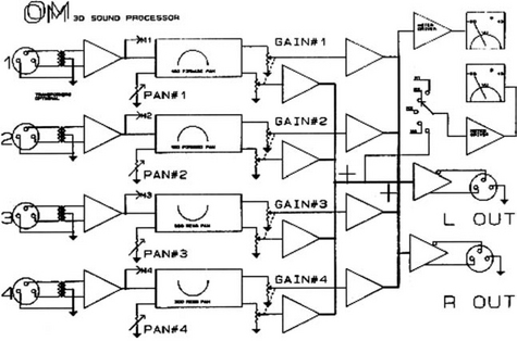

Figure 11.19 illustrates the maximum interaural time difference which may be generated by a hard-right panned signal in a conventional stereophonic arrangement. The signal is shown at the right ear delayed by t1 and at the left ear delayed by t2. The problem is trying to make a sound appear as if it is at position P. If it was, the signals would be as shown, with the left ear experiencing a signal delayed by t3. Figure 11.10 illustrates how this may be achieved. With the addition of an out-of-phase version of the signal at the left-hand loudspeaker, the interaural phase difference may be increased, thus generating the required perception. Unfortunately, if high frequencies were allowed to be emitted by the left-hand loudspeaker these would tend to recentralise the image because the ear is insensitive to phase for signals above about 700 Hz. So another approach has to be made. This may be illustrated by comparison with the monaural transfer functions of a sound approaching from 30° from the front (the true loudspeaker position) and the desired position (at 90° to the front). The monaural transfer functions for these two directions in the horizontal plane are given in Figure 11.21.

Figure 11.19 The maximum interaural time difference which may be generated by a hard-right panned signal in a conventional stereophonic arrangement
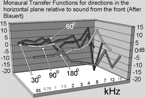
The required spectral modification (which must be made to the high-frequency signals emitted from the right loudspeaker alone – the other channel remaining mute) is derived by subtracting one response from the other. The clearest component is around 7 kHz which shows a pronounced dip at 30° and a marked peak at 90°. Note that at 60°, an intermediate level peak at the same frequency exists – suggesting that linear interpolation is justifiable. Furthermore there is a gradual rise in HF at the 90 degree position and another high-Q effect at about 10 kHz. Obviously conditions in the example given are generalisable to extreme left positions mutatis mutandis.
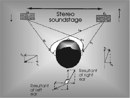
Figure 11.20 The addition of an out-of-phase signal at the ‘mute’ loudspeaker can be used to increase the apparent interaural phase difference
To implement such a technique electronically we require a panning circuit which operates over much of its range like an existing pan control and then, at a certain point, splits the signal into high- and low-frequency components and feeds out-of-phase signals to the loudspeaker opposite the full pan and spectrally modifies the signals emitted from the speaker nearest the desired phantom position. This is relatively easy to implement digitally but an analogue approach was taken in the development of OM so that the unit could be easily installed in existing analogue mixing consoles. The circuit for the OM panner is given in Figure 11.22. The circuit may be broken down into four elements: a variable equaliser stage; a gyrator stage; a conventional pan control (see next chapter) and a low-frequency differential mode amplifier.

The signal entering A1 is amplified by the complex ratio 1 + (Rx/Z1). Clearly this amplification is related to the setting of VR1a, which presents its maximum resistance in the centre position and its minimum at either end of its travel. Due to the impedance presented at the slider of VR1A, the frequency response of this circuit changes according to the control position. The function of CA is to provide a general high-frequency rise. Were it not for the imposition of the preset resistance PR1, the circuit would become unstable when VR1A was at either end of its travel. PR1 allows the degree of boost to be set as VR1A is moved from its centre position. CB, A2 and A3 and supporting components form a resonant acceptor circuit which resonates at the frequency the simulated inductance gyrator (L1) has the same reactance magnitude as CB. And where L1 is given by the expression:
PR2 sets, in the same way as PR1 did above, the degree of lift at the resonant frequency of CB and L1; this set to 7 kHz during test – as explained above. The signal that emerges from A1 is thus an equalised version of the input which acquires both general treble lift and specific boost around 7 kHz as the pan control is rotated in either direction away from the centre position. The degree of equalisation is adjustable by means of PR1 and PR2.
After the signal emerges from A1, it is fed to the relatively conventional panning control formed by Rp and VR1B. The impedances are so arranged that the output signal is – 3 dB in either channel at the centre position relative to extreme pan. A complication to this pan circuit are the capacitors strapped across each half of the pan control (Cp). These cause a degree of general high-frequency cut which acts mostly around the centre position and helps counteract the effect of the impedance at the slider of VR1A which still causes some equalisation, even at its centre position.
The signal then passes to A4 and A5, and associated components. This is an amplifier with a DC common mode gain of 1 and a DC differential gain of 2. The action of the 22 nF capacitors around the top leg of the feedback resistors is to limit the high-frequency differential mode gain to 1 while maintaining low-frequency differential gain as close to 2.
So, as the pan control is rotated to an extreme position, the differential mode amplifier gradually feeds low-frequency anti-phase information into the ‘quiet’ channel. At high frequency the differential mode amplifier has no effect but, instead, passes a high-frequency equalised version of the signal (with the few, salient auricle-coloration simulating high-frequency boost frequencies) to the left and right output. Figures 11.23 to 11.26 are oscillograms of typical output waveforms for a 400 Hz square-wave stimulus.


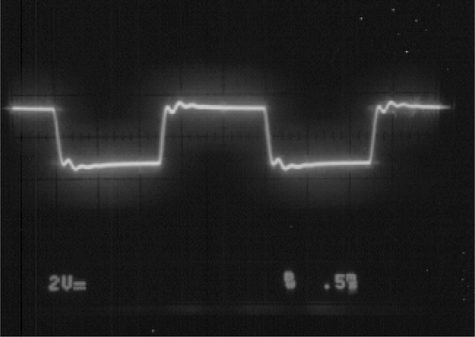
Figure 11.25 OM, dead channel, extreme pan (note opposite phase to waveform in Figure 11.24)

Figure 11.26 OM, both channels, centre rear (note majority of low-frequency information is out of phase)
The subsidiary circuit (formed around A6) follows the circuitry described above on the rear-pan channels. This was largely designed to accomplish a phase inversion on one channel at low frequencies. This technique facilitated a degree of mono compatibility. In effect, rear pan in the OM system was accomplished using a simple interchannel ratio technique on a signal which was largely composed of out-of-phase information at low frequencies. By adjusting the potentiometers which controlled high-frequency and high-Q boost appropriately it was further possible to create an appropriate attenuation of high frequencies in the rear arc – which is what is required from the psychoacoustic data. How this technique works is still not entirely known, its discovery being largely serendipitous. What is known is that head related movements reinforce a rear image generated this way and this is one of the most robust features of the OM system.
References
Bergault, D.R. 3-D sound for virtual reality and multimedia. Academic Press Inc., 1994.
Blauert, J. Spatial Hearing. MIT Press, 1983.
Brice, R. Multimedia and Virtual Reality Engineering. Newnes, 1997.
Edeko, F.O. (1988) Improving stereophonic image sharpness. Electronics and Wireless World, Vol. 94, No. 1623 (Jan.).
Malham, D.G. (1995) Basic Ambisonics. York University Web pages.
Nisbett, A. The Techniques of the Sound Studio. Focal Press, 1979.
Fact Sheet #11: An improved stereo microphone technique
What makes Blumlein’s 1933 ‘stereo’ patent (REF 1) so important is his originality in realising the principle (explained in Chapter 11) that interchannel intensity differences alone produce both high-frequency interaural intensity differences and low-frequency inter-aural phase differences when listening with loudspeakers. Intriguingly, Blumlein regarded the principle of pan-potted stereo as trivial – it seems, even in 1933, the principle of positioning a pre-recorded single mono sound-signal by means of intensity control was well known. The technological problem Blumlein set out to solve was how to ‘capture’ the sound field; so that directional information was encoded solely as intensity difference.
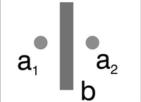
Blumlein noted that a crossed-pair of velocity microphones mounted at 45 degrees to the centre of the stereo image has the technological advantage that a pure intensity-derived stereo signal may be obtained from such a configuration without the use of electrical matrixing. His instinct proved right because this has become one of the standard arrangements for the acquisition of intensity coded stereophony, to such an extent that this configuration has become associated exclusively with his name, often being referred to as, the ‘Blumlein-pair’, an eponymous, and somewhat incorrect label! In fact, the greater part of Blumlein’s patent is concerned with a primitive ‘dummy-head’ (quasi-binaural) stereophonic microphone arrangement in which,
‘two pressure microphones a1 and a2 [are] mounted on opposite sides of a block of wood or baffle b which serves to provide the high frequency intensity differences at the microphones in the same way as the human head operates upon the ears’ (Figure F11.1).
Blumlein noted that, when listened to with headphones, the direct output from the microphones produced an excellent stereo effect but, when replayed through loudspeakers, the stereo effect was very disappointing. The transformation Blumlein required was the translation of low-frequency, inter-microphone phase differences into inter-channel intensity differences. He proposed the following technique:
‘The outputs from the two microphones are taken to suitably arranged network circuits which convert the two primary channels into two secondary channels which may be called the summation and difference channels arranged so that the current flowing in the summation channel will represent the mean of the currents flowing in the two original channels, while the current flowing into the difference channel will represent half the difference of the currents in the original channels…. Assuming the original currents differ in phase only, the current in the difference channel will be PI/2 different in phase from the current in the summation channel. This difference current is passed through two resistances in series between which is a condenser which forms a shunt arm. The voltage across this condenser will be in phase with that in the summation channel. By passing the current in the summation channel through a plain resistive attenuation network comprised of resistances a voltage is obtained which remains in phase with the voltage across the condenser in the difference channel. The voltages are then combined and re-separated by [another] sum and difference process … so as to produce two final channels. The voltage in the first final channel will be the sum of these voltages and the second final channel will be the difference between these voltages. Since these voltages were in phase the two final channels will be in phase but will differ in magnitude-only.
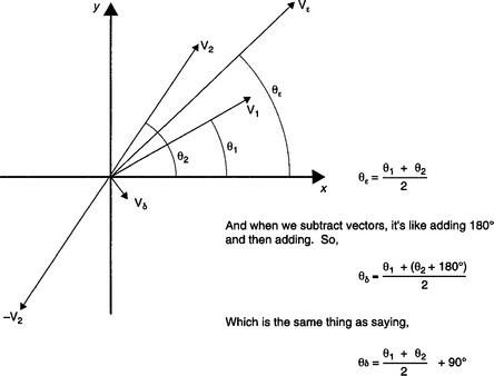
Blumlein’s comments on the perpendicularly of the sum and difference vectors are far from obvious. However, consider Figure F11.2.
A modern practical implementation
The circuit described below is designed so that maximum stereo obliquity is achieved when the inter-microphone delay is 500 μs. Other calibrations are possible mutatis mutandis. Table F11.1 below tabulates the phase-angle which 500 μs represents at various frequencies.
Consider the 30 Hz case. The circuit operates by first deriving the sum and difference of the phasor (vector) quantities derived from the primary left and right channels, i.e.
V2 = (sin 5.4 degrees, cos 5.4 degrees) = (0.1, 0.996)
So, at 30 Hz, the difference channel is 20 times (26 dB) smaller than the signal in the sum channel.
Now consider the situation at 300 Hz, where
at 300 Hz the signal is approximately 2 times smaller (6 dB) compared with the signal in the sum channel.
Now 300 Hz is nearly three octaves away from 30 Hz and the gain is 20 dB different demonstrating that the signal in the difference channel rises by 6 dB/octave. This confirms Blumlein’s statement that, ‘for a given obliquity of sound the phase difference is approximately proportional to frequency, representing a fixed time delay between sound arriving at the two ears.’
Looking now at the circuit diagram for the binaural to summation stereophony transcoder illustrated in Figure F11.3, consider the role of the integrator circuit implemented around U3a. The role of this circuit is both, to rotate the difference phasor by 90 degrees (and thus align it with the axis of the phasor in the sum channel) and to provide the gain/frequency characteristic to compensate for the rising characteristic of the signal in the difference channel. This could be achieved with a simple integrator. However, at intermediate and high frequencies (>1000 Hz), it is necessary to return the circuit to a straightforward matrix arrangement which transmits the high frequency differences obtained due to the baffling effect of the block of wood directly into the stereo channels. This is implemented by returning the gain and phase characteristic of the integrator-amplifier to 0 dB and 0 degrees phase-shift at high frequencies. This is the function of the 10 k resistor in series with the 22 nF integrator capacitor. (The actual circuit returns to 180 degrees phase shift at high frequencies – i.e. not 0 degrees; this is a detail which is compensated for in the following sum and difference arrangement.)

Clearly all the above calculations could be made for other microphone spacings. For instance, consider the situation in which two spaced omni’s (6 ft apart) are used as a stereo pick-up arrangement. With this geometry, 30 Hz would produce nearly 22 degrees of phase shift between the two microphones for a 30 degree obliquity. This would require,
that is, an integrator with a gain of 5. The gain at high frequency would once again need to fall to unity. At first this seems impossible because it requires the stand-off resistor in the feedback limb to remain 10 k as drawn in the figure above. However, consideration reveals that the transition region must begin at commensurately lower frequencies for a widely spaced microphone system (since phase ambiguities of >180 degrees will arise at lower frequencies) so that all that needs to be scaled is the capacitor, revealing that there is a continuum of possibilities of different microphone spacings and translation circuit values.
1For the engineer developing spatial sound systems such a clear, concise theory has many attractions. However, experiments devised to investigate the localisation of transient sounds (as opposed to pure tones) appear to indicate to most psychologists that the situation is a little more complicated than Lord Rayleigh had supposed. However, it may be demonstrated that their evidence supports Duplex theory as an explanation for the perception of the localisation (or lateralisation) of transients (Brice 1997).
2My original appreciation of this simple fact arose from a thought experiment designed to investigate the logical validity of the, oft cited, anecdotal preference among the golden-eared cognoscenti that vinyl records (and analogue recording equipment) can still offer a ‘lifelike’ quality unmatched by the technically superior digital compact disc. I reasoned that if I measured the differences between the signals produced from the pick-up cartridge and a CD player the signals would differ in several ways:
(i) The vinyl replay would have higher distortion and lower signal to noise ratio than its digital counterpart. There seemed little point in further investigating this aspect of recording and replay performance because so much work has been done on the subjective effects of dynamic range and linearity all suggesting, with very little room for error, that increased dynamic range and improving linearity correlate positively with improved fidelity and subjective preference.
(ii) The vinyl replay would have a frequency response which was limited with respect to the digital replay. This may play a part in preference for vinyl replay. It has been known since the 1940s that ‘the general public’ overwhelmingly prefer restricted bandwidth circuits for monaural sound reproduction.
(iii) Interchannel crosstalk would be much higher in the case of analogue recording and replay equipment. Furthermore, because crosstalk is usually the result of a negative reactance (either electrical or mechanical) this crosstalk would tend to increase proportionately with increasing signal frequency.
While attempting to imagine the subjective effect of this aperiodic crosstalk, it suddenly occurred to me that this mechanism would cause a progressive narrowing of the stereo image with respect to frequency which would (if it happened at the right rate) map the high-frequency intensity derived stereo image on top of the low-frequency, interaural delay derived image, thereby achieving the same effect as achieved by Edeko’s loudspeakers and Blumlein’s Shuffler circuit.
3The term quadraphonic is due only to the fact that the systems employed four loudspeakers; by implication this would make stereo – biphonic!