
Characterization of food materials in multiple length scales using small-angle X-ray scattering and nuclear magnetic resonance: principle and applications
Abstract:
Small-angle X-ray scattering (SAXS) and nuclear magnetic resonance (NMR) are state-of-the-art techniques commonly used to characterize the self-assembled structures and interactions of food materials at the nanoscale. This chapter covers the basic principles of SAXS, modern synchrotron facilities and the applications of SAXS in structure analysis of food ingredients. The principles and applications of several NMR-based techniques, including the diffusion research technique, spin relaxation technique and time-domain (TD)-NMR technique are also discussed.
6.1 Introduction
Food materials, which mainly consist of proteins, lipids and carbohydrates (including polysaccharides), are complex soft materials with length scales ranging from nanometer (i.e. micelles) to millimeter (i.e. foam of beer), and aggregation states ranging from dilute solutions (i.e. beverages) to concentrated solutions (i.e. salad dressing and butter) or gels (i.e. yoghurt). When investigating issues relating to interactions within multicomponent food systems, gel–sol transitions, phase separation, emulsion stability, etc., advanced experimental tools to characterize the structures and interactions of complex food systems on different length scales and time scales are required. In this chapter, the basic principles of using small-angle X-ray scattering (SAXS) and nuclear magnetic resonance (NMR) to characterize the structure of food materials are introduced. The applications of SAXS and NMR to determine the sizes and shapes of food biopolymers from form factors, interparticle interactions, structure factors and transport properties are then discussed in detail.
6.2 Small-angle X-ray scattering (SAXS): an introduction
Food systems are among the most complex soft materials studied by theoretical and experimental scientists.1 Although food systems are complex, they still follow the rules of modern physics of soft condensed matter. Modern technologies, including atomic force microscopy (AFM), dynamic light scattering (DLS), quartz crystal microbalance with dissipation monitoring (QCM-D), rheology, differential scanning calorimetry (DSC), etc., have been developed to better understand the structures and properties of food materials and interactions within them. Among those modern technologies, SAXS with third-generation synchrotron radiation provides us with a strong and convenient tool for probing the internal structures of those everyday soft materials. The X-ray scattering technique relies on the interactions of radiation with matter, like laser light scattering and neutron scattering. The differences between X-rays and other sources lie in their intrinsic properties (i.e. wavelength) and observation contrast (i.e. refractive index for laser and electron density for X-ray). The scientific use of X-rays began in the 1890 s. As gradual understanding of the basic theory of X-ray scattering developed over the next century, X-ray methods became more mature. During this period, more than 16 Nobel Prizes have been awarded for research into the interaction of X-rays with matter and their applications.2 Nowadays, X-ray related methods are used for a wide range of applications, including powder diffraction to determine crystal structure, circular dichroism to determine protein secondary structure, and X-ray imaging for medical applications.
The new generation of intensive X-ray synchrotron sources has accelerated the study of X-rays. Traditional X-ray facilities are usually limited to one wavelength and X-rays of low intensity, which make it time-consuming to conduct SAXS experiments. Compared to traditional X-ray sources, synchrotron sources that generate X-rays through the acceleration of charged particles radially have the advantages of high flux, small beam size, high stability, convenience and fast measurement. Among different X-ray technologies, SAXS has been applied to study structures with sizes from roughly 10 Å to several hundred Å. Most food biopolymers like food proteins and polysaccharides are within this size region. Laser light scattering in diluted systems provides information on hydrodynamic radius and size distribution. X-ray scattering serves as an excellent complementary tool to provide a systematic structural analysis involving overall shape, aggregation number, surface roughness, etc., for a rich variety of objects. SAXS will greatly help provide insight into the structures of food components and link this structural information with the macroscale mechanical, thermal and release properties of food components.
6.2.1 Basic principles of X‐ray scattering
Unlike normal light, X-rays can only provide us with a scattering pattern instead of direct information of the observed objects. The real information (i.e. particle size distribution) and scattering pattern follow the real-and-reciprocal rules, which give us the basic knowledge required to interpret the SAXS data. If R represents the real length of an object, then q, the scattering vector is in its reciprocal format. They satisfy R*q = constant, which can be 2π or 6/π.3 Since the development of scattering theory is based upon Bragg’s Law, let us take a quick look at the classical equation of Bragg’s Law, which is described as follows:
Distance d represents the repeated-order distance in the structure; λ, wavelength of the incident beam, is approximately 1 Å for X-ray beam; θ is the scattering angle. Small-angle scattering is very suitable for detecting biopolymers’ scattering patterns and structures. For instance, Pluronic PEO-PPO-PEO copolymer can form micelles with average sizes of approximately 10 Å. If you intend to view the repeated distance d with a value of 10 Å for micelle size calculation, the scattering angle θ should be lowered to less than 3°. For even larger biopolymers such as proteins and polysaccharides, it will need to be an even lower scattering angle. Therefore, small-angle scattering technology needs to be used to characterize those biomaterials with large-sized components.
Before going further, we need to understand the scattering vector q. The wave vector k of a monochromatic plane wave is defined as 2π/λ. Figure 6.1 shows the scattering triangle in which k0 is the wave vector of the incident beam, and k the wave vector of the scattered beam. The change between k0 and k is defined as scattering vector q. Here we only discuss the elastic scattering, that is, the energy of the beam does not change during scattering. Therefore, the wavelength λ of k0 is equal to that of k. Then we can easily get another basic equation for describing scattering vector q.
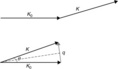
Fig. 6.1 Scattering triangle of wave vectors for incident beam k0 and scattered beam k, and scattering vector q. 2θ: scattering angle.
Substitute Equation 6.1 into Equation 6.2, we can obtain the following reciprocal relationship:

Equation 6.3 once again displays the real-and-reciprocal rule embedded in SAS technology. From Equation 6.3 it is once again demonstrated clearly that the small-angle method is suitable for viewing large-scale objects, especially food ingredients such as proteins and polysaccharides.
6.2.2 Modern synchrotron X-ray facilities
It is usually difficult for conventional X-ray facilities to undertake SAXS experiments due to beam divergence and wavelength limitations. With the development of modern synchrotron radiation, SAXS has been rejuvenated as a very powerful tool for applications in physics, biology, chemistry and materials science. Currently, there are more than 35 synchrotron SAXS beamlines worldwide, including those located in the Photon Factory at High Energy Accelerator Research Organization in Tsukuba, Japan; Advanced Photon Source (APS) at Argonne National Lab in Illinois, USA; Laboratoire pour l’Utilisation du Rayonnement Electromagnétique (Lure) in France; and National Synchrotron Light Source (NSLS) at Brookhaven National Laboratory in New York, USA.4 With the increasing demand for structure analysis in different scientific disciplines, new synchrotron facilities have recently opened, such as the Shanghai Synchrotron Radiation Facility (SSRF) in China, which was opened to general users in May 2009, and the ALBA synchrotron facilities in Cerdanyola del Vallès, Spain, which was put in use in 2010.
Modern X-rays are generated from a highly vacuum-circulated electron beam accelerator. The bending trajectory along which the charged particles travel helps with the emission of X-rays. This modern X-ray is much more intensive than that provided by traditional X-ray tubes, usually with many orders higher intensity. Such a high flux beam greatly shortens the period of experimental measurement. Figure 6.2 displays the schematic diagram of a synchrotron radiation circular accelerator. There are several major components installed in the storage ring, including an injection system, a vacuum chamber, bending magnets, focusing magnets and undulators. The injection system generates electrons prior to particle acceleration. Both bending magnets and focusing magnets are utilized to bend the trajectory of the generated electrons. Compared with bending magnets, focusing magnets are applied to tune the electron beam path in a more refined manner. Long vacuum chambers are utilized to transport the electron beam with very limited energy loss. Undulators keep the X-ray beam’s high intensity with narrow energy bands in the spectrum along the beamline. Afterwards the generated X-ray beams are transported to different sites around the large acceleration ring for different applications. SAXS is usually among those different synchrotron X-ray technique tools. Figure 6.3 shows the representative scheme of SAXS at BioCAT-18ID beamline at the Advanced Photon Sources (APS), Argonne National Laboratory, USA. Different accessories are attached along the beamline to ensure the high quality of beamline output for SAXS experiments.5 Long adjustable vacuum chambers guarantee sample-to-detector distances from 100 to almost 6000 nm, which covers the q range from ~ 0.001 to ~ 30 nm- 1. The guard slits are applied to reduce parasitic scattering. Double focusing optics decrease focal spot sizes to approximately 150 × 40 μm2. The 18ID beamline is equipped with a high-sensitivity charge coupled device (CCD) detector with large working area and high spatial resolution. SAXS is often applied to test biological macromolecules such as a dilute protein solution. In order to avoid the sample damage caused by a high flux of beamline, a temperature-controlled water-jacketed flow cell has been designed for the bio-sample chamber.
![]()
Fig. 6.2 Schematic diagram of modern synchrotron radiation facility. The closed circuit is the storage ring for electron acceleration. IS, injection system; RF, radiofrequency cavity; L, beamline; BM, bending magnets; FM, focusing magnet Reproduced with kind permission from Ref. 6; © Oxford University Press.
![]()
Fig. 6.3 Schematic representation of the synchrotron X-ray scattering BioCAT-18ID beamline at the APS, Argonne National Laboratory, USA: (1) primary beam coming from the undulator, (2) and (3) flat and sagittaly focusing Si (111) crystal of the double-crystal monochromator, respectively, (4) vertically focusing mirror, (5) collimator slits, (6) ion chamber, (7) and (8) guard slits, (9) temperature-controlled sample-flow cell, (10) vacuum chamber, (11) beamstop with a photodiode, (12) CCD detector Reproduced with kind permission from Ref. 5; © Institute of Physics Publishing.
6.2.3 Comparison of SAXS and small‐angle neutron scattering (SANS)
Similar to SAXS, small-angle neutron scattering (SANS) is also frequently utilized for probing materials structures. Most of the time, particles in X-rays and neutrons share similar properties so many theories and experiments developed with X-rays can be applied to neutron scattering. However, there are some important differences that make these two methods complementary to each other. For instance, with regard to the particle aspect of wave–particle duality, the energy of a neutron particle is in the order of 103 keV but that of an X-ray photon is only in the order of 10 keV.6 The similarity between the energy of neutron particles and the kinetic energy of atoms’ motion allows SANS to easily detect the energy exchange between atomic motion and neutron particles. Herein we have called scattering involving energy exchange inelastic scattering. Thus the measurement of inelastic neutron scattering can be a very helpful method for detecting atomic motions in materials. However, we do not plan to discuss inelastic scattering between neutrons and atoms because it is beyond the scope of this chapter. We only focus on elastic and coherent scattering and mainly on SAXS, in part because the SAXS itself can provide us with a lot of structure information. The ease of sampling also makes SAXS experiments convenient to conduct.
6.3 Direct and indirect interpretation of SAXS data
Since X-rays can only provide us with indirect information about material structure, we need analytical methods to interpret SAXS patterns and transform those patterns into real-space information. One of the most important concepts is the scattering length density distribution ρ(r), which indicates the number of electrons per unit volume. When an incident beam hits an obstacle, the obstacle will generate a fresh secondary wave. Equation 6.4 shows the relationship between scattering amplitude A(q) and the scattering length density ρ(r). The phase information of the wave function is presented by the term e− iqr, which can also be understood as the Fourier transform of the scattering length density ρ(r).
However, it is the scattering intensity I(q) rather than the amplitude A(q) that can be directly measured through experiments:
Nevertheless, Equation 6.5 is still not straightforward enough for further analysis. Through mathematic derivation by Debye (1915),7 we substitute the phase term e− iqr by sin qr/qr. Then we obtain the basic Debye function as Equation 6.6:
Furthermore, sin (qr)/qr can also be substituted by the Maclaurin (or Taylor) expansion. sin(qr)/qr ≈ 1 − (qr)2 /3! + · · ·. Therefore, the scattering equation can be derived into a polynomial function, which becomes easier to solve for the parameters related to structure and interaction of materials. In addition, we can modify the original scattering function by coupling it with different classic physical models to match the particles with known shapes. For convenience, we take an example of a dilute system where interparticle interactions can be ignored, with particles in different geometries. We wish to determine the shape and size of the particles in the matrix using SAXS. For instance, let us take a close look at a dilute dispersion of solid spheres with radius R and uniform electron density ρ0. We integrate the Debye function with the upper limit R and the bottom limit 0. Then we can easily obtain the scattering function of a solid sphere.
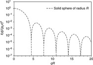
Figure 6.4 exhibits the scattering intensity I(q) profile of a solid sphere with radius R. It is worth noting that this is a semi-log plot, which shows the characteristic of wave function although one cannot observe this feature when log–log scale is applied. Since macromolecules can self-assemble into different shapes, we should apply a uniform concept for comparison. Radius of gyration, Rg, a concept from polymer science, is applied for each type of particle of different shapes. To compare the effects of particle shapes on their scattering profiles, we fix the Rg value. Four typical types of ordinary particle geometries, including sphere, thin rod, circular disk and random coil, are taken into consideration. The relationship between Rg and sphere radius R, rod cross-section radius R′, length L, and circular disk radius R″ can be found in the references by LaRue et al., Li, and Kroy et al.8-10 The detailed procedure to build these models can be found here.6, 7
In Fig. 6.5, four typical scattering curves for solid sphere, rod, disk and random coil have been illustrated. It is easily found that at low q region, these curves overlap with each other. It seems that we can utilize one method to analyze the SAXS data at low q, which is convenient for real manipulation. This convenient analysis tool is called Guinier law or Guinier fit. 11 The typical Guinier equation is shown as follows.
With the Guinier plot, we can determine the radius of gyration Rg of a particle with unknown shape and size. However, the Guinier law is only valid when the following three conditions are satisfied: (1) qRg < 1; (2) dilute system without interaction of particles; and (3) isotropic feature without specified orientation. For condition (1), if qRg > 1, scattering curves of different geometrical particles will develop in different trends. For concentrated samples, light interference among particles cannot be avoided and then the structure factor S(q) is not 1 anymore, where I(q) = φVp (Δρ)2 P(q) S(q). Then the normal Guinier plot will not be suitable for application. From the above rules, we can summarize the procedure to obtain Rg through Guinier fit as follows: (1) estimation of Rg; (2) selection of the region when qRg < 1; and (3) obtaining final accurate Rg.
Besides, the homogeneity of protein conformation entrapped in polymeric micelles can be determined by the SAXS peak profiles in middle q region as well.12 Through comparison of different scattering profiles, we may extract the structure information from large q region. Large q in reciprocal space responds to small-scale information of macromolecular chains. Within this q region, the morphology and rigidity of polymers can be obtained by the Kratky-Porod method.13 In Fig. 6.5, the intensity I(q) follows different scaling rules of I(q) ~ q− α. The exponent α is different, depending upon particle shapes, for example, 4 for solid sphere, 2 for disk and random coil, and 1 for rod. In most cases, the nanoparticle solution combines the features from both random coil and other geometries like rod since polymer chain has its own rigidity and conformation in reality.
For convenience, we introduce persistence length lp, indicating the stiffness of polymer chain. If the observed length r is larger than lp, the object may behave in a flexible manner like random coil. However, if the observed length r is less than the persistence length lp or r < lp, the object will show more rigid features like rod. Because it is sometimes not very clear for readers to recognize the exponent α, Kratky plot [I(q)q2 ~ q] is then employed to verify the rigidity of polymer chain in the system, as shown in Fig. 6.6. The q value at the transition between two different q regions has an inverse relationship with persistence length lp. Portnaya et al. utilized Kratky plot to interpret the SAXS profile of β-casein at low pH and low ionic strength condition.14 From the Kratky plot, the self-assembly of β-casein at low pH condition was found to be an intermediate state combining globular and random coil structures. Portnaya et al. named this kind of conformation of β-casein as an intermediate pre-molten globule with some residual structures.14 In terms of direct analysis, the combination of mathematic derivation, Guinier law and Kratky-Porod method can be applied to extract the structure information from original scattering profile.
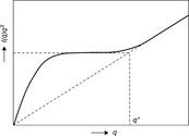
Fig. 6.6 Kratky plot ofa single polymer chain in different Q regions Reproduced with kind permission from Ref. 6; © Oxford University Press.
Equations 6.8–6.11 give us the usual equations applied for particles with different geometries. Equations 6.8, 6.9, 6.10 and 6.11 represent globular, rod-like, disk, and random coil conformations, respectively.
R: radius of sphere, J1 is the first order of Bessel function written as
L: length of rod, the cross-section area can be omitted. Si is the sine integral function.
R: radius of disk, thickness can be omitted.

Although these direct analytical methods are easy to use, they have their own limitations. For example, the application of Guinier Law is quite sensitive to the low q data. Therefore, the radius of gyration (Rg) extracted from Guinier fit may not be very accurate. Other indirect transform methods thus need to be employed to ensure more accurate structure estimation. The accuracies of Rg obtained from both Guinier fit and indirect Fourier transform developed by Glatter in 1977 have been compared in previous literature.15 It is shown that the indirect methods can provide more precise Rg without depending on limited low q data. Basically, these indirect methods provide convenient conversion from reciprocal profile of I(q) ~ q to real-space size distribution of P(r) ~ r. The function of P(r) is named as the pair distribution function (PDF) which represents the probability of finding a pair of particles within the shell at distance r. The real-space PDF curve contains similar information as the direct methods mentioned above, and the real-space curve is more straightforward and informative.
There are many approaches to analyze SAXS data through indirect Fourier transform, such as Glatter, 15 Moore,16 Provencher’s17 and other regularization methods that have been proposed. These approaches are the basis for software development to automatically interpret SAXS data. There are two popular programs for direct structure analysis, including GNOM and the Irena package embedded in the commercial software Igor Pro. Many SAXS analyses of protein or polymeric micelle solution involve Fourier transform performed by the program GNOM.18 Basically, GNOM was developed based upon Tikhonov’s α regularization technique, which is designed to solve ill-posed problems. Finding a suitable regularization parameter α is of vital importance to perform Fourier transformation and curve fitting by GNOM.19 The perceptual criteria are utilized to ensure the reasonable estimation of parameter α. The criteria herein include DISCRP, OSCILL, STABIL, SYSDEV, POSITV and VALCEN. Each criterion has different meanings. For instance, OSCILL displays the smoothness of the solution while STABIL exhibits the solution stability under the fluctuation of parameter α. The values of these criteria give direct evaluation of the solution quality. Evaluation of those criteria prior to determining the right regularization parameter α can be found in the literature of Svergun et al.19 For instance, PDF curve with the values of OSCILL 1.1, POSITV 1 and VALCEN 0.95 will be stable and reliable while the values of OSCILL 2.26, POSITV 0.99 and VALCEN 0.95 only reflect unstabilized PDF results.
Another program package Irena is developed embedded in the software Igor Pro by Wavemetrics Inc. Compared with the GNOM package, Irena package integrates many other functions such as data refinement, regularization and pair–distance distribution function together. For PDF curve generation, both regularization and Moore’s indirect Fourier transform are included in this Irena package.20 The difference between the above two methods lies in the fact that Moore’s method optimizes the maximum dimension Dmax.20
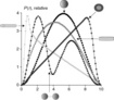
It is strongly suggested that we should apply multiple methods to analyze SAXS data to ensure the accuracy of data analysis. Through PDF curves’ contours, we can notify what sort of shape the sample belongs to. Figure 6.7 shows typical PDF of different geometrical particles with the same maximum dimension Dmax.5 Globular particles present P(r) function curve with bell shape and the peak is located at approximately Dmax/2. Thin rod or elongated particle has a skewed scattering profile with a peak located at small distance, indicating the rod’s cross-section radius. Disk’s curve is a broadened bell curve of globular particles with a peak at position smaller than Dmax/2. The peak of a hollow particle’s PDF curve shifts to the distance larger than Dmax/2 compared with globular particle. Sometimes particles have inner structures and therefore we can get different intra-distances from PDF curve, displaying both the major size and distance between subunits. It is also possible to gain high-resolution atomic bonding distances such as bonding distances between C, N and O atoms.21 Besides, it should be noticed that all these PDF curves for particles of different geometries are gained from empirical experiments. Further efforts in PDF research are needed to recognize the geometry of unknown structures.
6.4 Application of synchrotron SAXS to food materials
Synchrotron SAXS is a powerful tool for probing the internal structure of soft matter. Research targets like food proteins or polysaccharides, polymeric micelles, protein unfolding, protein–polysaccharide interaction and protein–active compound interaction are all challenges for structure investigation by synchrotron SAXS techniques. These topics cover different research demands in the food industry. For instance, biopolymer-based micelles have been proven to work quite well as wall materials to enhance the bioavailability of insoluble compounds such as curcumin, which provides us with novel functional food ingredients for healthy food products.22 However, to thoroughly characterize individual food components such as proteins and polysaccharides, polymeric micelles, or the interactions between proteins and other macro/micro compounds, the combination of SAXS with various traditional techniques is necessary to provide precise description. The techniques generally used to combine with SAXS include scanning probe microscopy (SPM) for morphology, dynamic light scattering (DLS) for particle size of isotropic system, pendant drop goniometer for surface tension of synthetic surfactant, etc. Rieker et al. explored the complementary roles of SAXS and transmission electron microscopy (TEM) for concentrated hard sphere systems.23 They proved that fitting the Porod region of SAXS data to form factor of hard spheres produced accurate estimation of the mean particle size and polydispersity.23
6.4.1 Food proteins and polysaccharides
Proteins and polysaccharides are major components in food. Their structures at the microscale have a great impact on macroscale properties including texture, viscosity and mouth-feel. For instance, in most dairy products such as yoghurt and ice cream, the ingredient carrageenan forms a helix structure when interacting with casein to prevent casein micelle from macroscopic phase separation, which gives the finished products a smooth and thick mouthfeel.24 Probing the inner structure of those food biopolymers such as proteins and polysaccharides helps modern food scientists to precisely design novel functional food products. Therefore, the combination of synchrotron SAXS technique with basic biomaterials structural analysis methods will be powerful for novel food product design in the future. What is more, the structures of proteins and other biopolymers like DNA, RNA are always important research topics. In 2009 alone, the National Institutes of Health (NIH) spent $80 million on the Protein Structure Initiative.25 As a complementary technique to X-ray diffraction, which requires highly crystallized samples, many research groups have utilized SAXS to determine polymeric crystal structures in soft matter. Shamai et al. applied SAXS to determine the colloidal structure of native high amylase corn starch and polymorphs of resistant starch type 3 (RST 3).26 The RST 3 attracted much attention due to the fact that it maintained nutritional functionality during the cooking process. Shamai et al. studied the polymorphism of high amylase corn starch tuned by different retrogradation temperatures. Modified lamellar model was applied to fit SAXS curves for samples under low temperature. Although the long-range periodicity was observed, the overall crystallinity was quite low in the granular form. Retrogradation at high temperature resulted in a mixture of polymorphs A and V. The dilute system of individual lamella was applied to fit the SAXS data of high-temperature samples. The structure difference between low-temperature and high-temperature samples lies in the amount of bound water molecules. The formation of polymorph A and V at high temperature results from fewer bound water molecules than those in low-temperature samples. Pitkowski et al. also utilized SAXS to determine the structure of casein before and after polyphosphate dissociation,27 and they observed the difference in casein structure before and after dissociation. Forato et al. performed Guinier analysis and PDF profile to determine the structure of Z19 protein, an important fraction of α-zein.28 Afterwards, they proposed the hair-pin model based upon the SAXS data and the computational models from GASBOR. The difference between their SAXS analysis and the previous results by Tatham et al. lies in the fact that α-helix structure of Z19 was extended upon environmental changes rather than the change of folding itself. Their analytical procedure has been applied to study prolamins such as oat prolamin, hordein from barley and pennisetin from pearl millet.28 The low-resolution structural model is proposed to determine the pH effect on the structure of porcine pepsin by Jin et al. based upon the different analyzed dimensions and DAMAVER program.29 They established the structure model without imposing any restrictions on the symmetric conformation of the pepsin molecule. Their model was similar to the core–shell nanoparticle model. The environment-dependent chain stretching of C-terminal domain greatly influenced the molecular flexibility rather than the rigid and folded core parts in the N-terminal domain. SAXS can also contribute to high-resolution atomic structure modeling. Hong et al. applied the combination of SAXS and WAXS (wide-angle X-ray scattering) to obtain a scattering profile covering a wide range of scattering vector.21 They succeeded in finding the peaks locating in the low distance region of PDF curve [P(r) ~ r] of bovine erythrocyte hemoglobin in sterile phosphate-buffered saline solution; they correspond to the average bond length between C, N and O atoms and the distance between adjacent α-helixes. The direct fast Fourier transform (FFT) also verifies the true occurrence of those peaks in P(r) ~ r plot. To sum up, SAXS studies in biopolymer solutions are very important, especially under the situation where proteins and polysaccharides are very difficult to crystallize. Synchrotron X-ray scattering provides us with a sound method to probe different hierarchical structures of those biopolymers and their conformation alternations under different situations.
6.4.2 Food-level polymeric micelle
Polymer micelles play an important role in colloidal science due to their wide range of applications. These micelles usually have hydrophilic/hydrophobic blocks, which facilitate the formation of a stable water–oil interface. These amphiphilic polymers are capable of reducing the interfacial energy between oil and water and thus are usually used as surfactants in emulsions, drug delivery and nutraceutical encapsulation systems. The micelle structures have a large impact on the stability and the release profile of different delivery systems under different conditions. Probing the structures of polymeric micelles helps food scientists achieve the control release of active compounds from micelles. Different structure information such as size, shape and bonding length can be extracted from SAXS profiles of micelle solutions. Yu et al. utilized hydrophobically modified starch (HMS) to encapsulate curcumin, which is a traditional anti-cancer compound with the disadvantage of low bioavailability.22 The results from human heptocellular cell line HepG2 proved curcumin’s improved anti-cancer activity by HMS encapsulation. In addition, Yu et al. applied SAXS to determine the structure alternation before and after the addition of HMS. Through the fitting of SAXS scattering profile from dilute solution using Debye function, the radius of gyration (Rg) of starch or HMS remained unchanged, which illustrated that the addition of curcumin would not affect the micelle structure of HMS. Indeed, SAXS can provide more complicated information of polymeric micelles than just discussed. Akiba et al. successfully synthesized a partially benzyl-esterified poly(ethylene glycol)-b-poly(aspartic acid) [PEG-P(Asp(Bzl)] and applied PEG-P(Asp(Bzl) to load a hydrophobic retinoid antagonist drug.30 In their paper, SAXS was an in situ technology to observe drugs in the core directly. A diffraction peak locating at q = 4 nm–1 was found to attribute to the distance between α-helixes. When the hydrophobic drug was added, this diffraction peak disappeared, indicating the homogeneous distribution of this hydrophobic drug. In order to further analyze the SAXS data, Akiba et al. applied core–shell spherical micelle model to fit the original data. Through the core–shell model, they found that the core radius increased sigmoidally from 5.9 to 6.9 nm by the addition of drug into core while the thickness of shell maintained similar values. Two factors including osmotic free energy and attractive interaction contributed to the sigmoidal-shape increase of core radius. The specific number of polymer chains in single micelle varied from 145 to 182. Shrestha et al. applied SAXS to study systematically the effects of solvent, temperature and concentration upon the structure of glycerol α-monomyristate (C14G1) micelles.31 Different from previous examples, C14G1 formed reverse micelles in different organic solvents at relatively high temperatures up to 70 °C. The shape, Rg and Dmax from PDF curves of C14G1 reflected the structural change under different conditions. Long chain oil such as hexadecane prompted C14G1 to shape into long cylinders from short rods, verified by the shift of the major peak positions and Dmax to the large distance values. The increase of temperature resulted in the shrink of C14G1 micelle, which was explained by the increased oil penetration capability upon the increase of temperature. From similar PDF analysis, concentration increase led to one-dimensional increase of rod length, which ensured thermodynamic stability at the cost of excess free energy. They also checked the influence of polar solvents such as water and glycerol on micelle structure. Larger forward scattering intensity [I (q = 0)] and overall shift of PDF curves reflected the fact that water molecules were apt to form water pools at the micelle core. In terms of novel biopolymers in aqueous system, Huang et al. succeeded in synthesizing octanoylchitosan-polyethylene glycol monomethyl ether (acylChitoMPEG) which was used as a novel bio-amphiphile.32 Their complete SAXS analysis, including PDF curves from GNOM, micelle aggregation number gained from forward scattering and core–shell structure fitted by Pedersen’s core–chain model,33 greatly helped them establish the coiled structure model which was composed of triple helical acylChitoMPEG chains in single coil.32
6.4.3 Interaction between proteins and other compounds
The interaction between proteins and other bioactive compounds is a critical research topic in modern colloidal chemistry. Protein–active compound interaction is usually directly related to practical problems occurring in the food industry as well. Understanding how to control or limit their occurrence requires internal structure information on the atomic level. SAXS is a fairly suitable tool for addressing these food-related problems. For example, the astringency of tea, red wine, beer and chocolate, which is a complicated sensation, is directly relevant to the interaction between tannins and saliva proline-rich proteins (PRP). The tannin-induced precipitation of those PRP causes a loss of lubrication in the oral epithelium.34 Jobstl et al. investigated the binding of β-casein and epigallocatechin gallate (EGCG) as a model system for tannin-induced PRP aggregation since β-casein and PRP have similar conformation in dephosphorylated form.35 Individual β-casein behaved like a random coil. When EGCG was added into the β-casein matrix, β-casein formed spherical and ellipsoidal structures at low or high EGCG/protein ratios, respectively. Those structural alternations can be observed through Kratky analysis and PDF curves based on SAXS measurements. NMR PGSE (pulsed-gradient spinecho NMR technique) experiments were also applied to determine the diffusion coefficient and hydrodynamic radius of β-casein,35 which illustrated that the combination of NMR and SAXS provided complete structure information for a given target. NMR-related technologies will be illustrated in detail in the second part of this chapter. After Jobstl’s relatively early publication, other researchers utilized SAXS to probe EGCG/PRP binding and its inhibition. Pascal et al. studied the protein concentration and polyphenol/protein ratio effect upon human proline-rich protein/EGCG interaction.34 During Pascal’s studies, he first investigated the binding between non-glycosylated human PRP (IB-5) and EGCG by using DLS, isothermal titration microcalorimetry and circular dichroism. The three-stage model was applied to explain the binding process, which included saturation of binding sites, protein aggregation and phase separation. Then based upon the SAXS profiles of EGCG-glycosylated PRP mixtures, Pascal et al. proposed a model for proteintannin aggregation, which obeyed an aggregation equilibrium similar to a micellization equilibrium.36 The interactions between EGCG and PRP were attributed to hydrophobic interaction and hydrogen binding, which suggested how to avoid those unnecessary bindings by adding ethanol to reduce hydrogen binding.
Another example is relevant to food allergy. Much research has focused upon the mechanisms of food-induced allergy like hypersensitivity induced by glycinin, a soybean protein. The structures of glycinin under different conditions such as pH, salt and dry or wet state were probed by SAXS.37 The structure information obtained from SAXS profiles of protein in powder and solution states allowed us to design food ingredients with improved stability, shelf life and sensory properties. Powder scattering profile indicated the long-range order structure by protein crystals. Solution scattering profile reflects the protein self-assemblies under different pH conditions, which precipitate at pH 5 near pI, denatured breaking-down at pH 2 and denatured aggregation at pH 11. Understanding structures of disease-related proteins such as glycinin provides us with the structure mechanism behind disease phenomena. Recently, it has been demonstrated through in vivo rat model that lipoic acid effectively reduced mast cell numbers, the level of serum IgE and the level of histamine release.38 However, the structural mechanism behind the phenomenon is still unclear. SAXS is a promising tool to address this problem in the future.
6.5 Nuclear magnetic resonance (NMR)
An NMR facility was initially developed in 1946 by researchers at Stanford University and Massachusetts Institute of Technology. The advances in radar technology during World War II accelerated the development of the NMR spectrometer. In the following 50 years, NMR became a prominent organic spectroscopy used by chemists to determine the structures of various synthetic compounds. Prior to a description of the principles of NMR itself, the concept of “spin” is introduced for further understanding of nuclei behavior in magnetic fields. The particles which assemble into nuclei such as protons, neutrons and electrons can spin. Their spin behaviors are affected by external magnetic fields. Different nuclei have distinct spin behaviors in magnetic fields, which can be quantified by NMR spectrometry. Proton (1H) spin is the behavior most frequently utilized in NMR investigation due to its abundance and high resolution. In addition to external magnetic field, nuclei spins can also be perturbed by electromagnetic pulses. Different molecules have different feedback towards the magnetic field and pulse perturbation which change their nuclei magnetic momentums. Additional pulse perturbation for different molecules will generate different free induction decay (FID) signals (a time-domain signal when nuclei magnetic momentum goes back to equilibrium upon pulse perturbation). After being processed using Fourier transform, the time-domain (TD) signals can be transferred to the frequency-domain signals which are more frequently observed during daily NMR experiment. Generally, there are two types of NMR instruments: continue wave and Fourier transform. The continue wave instrument which was used in the early days shares the same principle as conventional optical-scan spectrometers. By contrast, the Fourier transform instrument is currently the more accepted type. Its principles have been described above.
With the fast-paced development of both theory and facilities, NMR has been utilized for different applications including medical research. The follow discussion will focus upon some representative NMR techniques for colloidal and soft matter characterization. Several categories of NMR including molecular diffusion, spin relaxation and time-domain NMR will be covered. Several techniques from each category and their applications are detailed below.
6.6 Diffusion NMR
Pulsed-field gradient (PFG) NMR has been widely used in the study of particle diffusion and particle size distribution in a variety of liquid systems. There are several PFG-NMR techniques that can be utilized for particle diffusion determination, including standard spin-echo pulsed-field gradient (SE-PFG) NMR, stimulated SE-PFG NMR and droplet diffusion. The following sections provide a basic introduction to these PFG-NMR techniques and their technical applications.
6.6.1 Pulsed-field gradient (PFG) NMR
Standard spin-echo pulsed-field gradient experiment
In standard SE-PFG NMR, molecular displacement along the gradient direction leads to the attenuation of the echo signal. Figure 6.8 shows the schematic of standard SE-PFG NMR. This process is described by Equation 6.12, which is used to obtain the self-diffusion coefficient.39
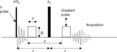
Fig. 6.8 Schematic of standard spin-echo pulsed field-gradient experiment (SE-PFG) Reproduced with kind permission from Ref. 39; © American Chemistry Society.
I0 is the intensity of the signal immediately after the 90x° pulse,τ is the time interval between the 90x° and 180y° pulses, Δ is the duration between the leading edges of the gradient pulses, T2 is the spin-spin relaxation time, δ is the length of the gradient pulse, D is the self-diffusion coefficient, and γ is the gyromagnetic ratio. For a proton, the gyromagnetic ratio is 26.752×10⁷ rad T–1 s–1. The SE-PFG method is often used in the situations where the spin–spin relaxation time is not too short compared to the diffusion time.
Stimulated spin-echo pulsed-field gradient experiment
Stimulated spin-echo pulsed-field gradient experiment (STE-PFG) NMR is a more commonly employed derivative of the PFG method.39 In a STE-PFG sequence, the excitation time is made up of two parts, a shorter time (τ) during which T2 relaxation occurs and a longer time (T) in which T1 relaxation happens. This method greatly extends the diffusion time for the situation when T2 is short but T1 is long. The signal attenuation in a STE-PFG experiment is described in Fig. 6.9.
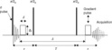
Fig. 6.9 Schematic ofstimulated spin-echo pulsed field-gradient experiment (STE-PFG) Reproduced with kind permission from Ref. 39; © American Chemistry Society.
Each letter or symbol in Equation 6.13 is used in exactly the same way as in Equation 6.12. Equations 6.12 and 6.13 are only valid for “free” molecular diffusion. The more complicated equation developed by Murday and Cotts40 using the GPD approximation41 needs to be applied for the situation where molecular diffusion is restricted by physical boundaries, as shown in Equation 6.14.
αm is the mth root of the Bessel equation, J3/2(αa) = αa J5/2 (αa). Additionally, in Equation 6.14, the decays that are due to spin relaxations are not considered, therefore S0 is the initial intensity in Equations 6.12 and 6.13, simultaneously including the relaxation terms.
In Equation 6.14, the only free parameter is the emulsion droplet radius “a” and all the other parameters are derived by execution of the experiment. Compared with alternative droplet sizing techniques (e.g. light scattering, optical observation, ultrasound spectroscopy and electrical conductivity measurement), NMR emulsion droplet sizing is capable of testing very concentrated emulsions and is completely non-invasive. For NMR diffusion technique, higher droplet concentrations will give improved particle size results due to the increased signal-to-noise ratio. This feature makes NMR diffusion method directly applicable to the sizing of droplets in emulsions in which particle sizing is beyond the capability of other methods.
6.6.2 Droplet diffusion
Application of Equation 6.14 assumes that the Brownian motion of droplets is negligible, which is true in a concentrated system. However, in a dilute system, this is not always the case.39 In a dilute spherical particle suspension, the diffusion coefficient can be described by the Stokes-Einstein Equation:42

where k is the Boltzmann constant, T is the temperature and η is the viscosity of the surrounding fluid.
The diffusive attenuation of the NMR signal in emulsion droplets is usually due to the combination of both restricted molecular diffusion within droplets (Equation 6.14) and the droplet diffusion themselves (Equation 6.15). This was written in detail by Garasanin et al.39 Generally, for emulsion droplets larger than 1 μm, the effect due to droplet diffusion is negligible, and the droplet diffusion effect is also significantly reduced in concentrated systems.
6.6.3 Determination of phase transition boundaries in nanoemulsions
The variation of amounts of either water or oil in nanoemulsions usually leads to phase transition from O/W (oil in water) to W/O (water in oil) or W/O to O/W, and sometimes a bicontinuous phase also exists. Phase transition investigation is highly meaningful for nanoemulsions. The complete transformation from one phase to another can occur gradually or progressively as the amount of water or oil changes. It is not always easy to clearly define the transition boundaries within one phase diagram from traditional techniques, such as viscosity measurement. The PFG-NMR technique provides an easy and straightforward way to define the transition boundaries and to estimate the effect of solubilizates on the phase transitions. In PFG-NMR, phase transition of emulsion results in different relative diffusion coefficients of water or oil.
Figure 6.10 shows the transition from W/O phase to bicontinuous phase in microemulsions with phytosterols and lycopene.43 The diffusion coefficient of water (Dw) was normalized to the values measured for the aqueous phase (water/polyol, D0w = 55.5 × 10 − 11) and was plotted against the aqueous phase content in microemulsions containing phytosterols (Fig. 6.10a), and lycopene (Fig. 6.10b). Diffusion coefficients of empty emulsions were measured as the control. The diffusion coefficients of water in the W/O region are quite different in empty and solubilized systems.
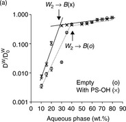
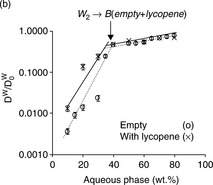
Fig. 6.10 Relative self-diffusion coefficients ofthe water (Dw/D0w) calculated from PGSE NMR (pulsed gradient spin echo NMR) as a function of aqueous phase content in the R-(+)-limonene–ethanol–water–PG systems based on Tween 60 of empty microemulsions (![]() ) and microemulsions loaded with nutraceuticals (×): (a) phytosterols as guest molecule, and (b) lycopene Reproduced with kind permission from Ref. 43; © Royal Society of Chemistry.
) and microemulsions loaded with nutraceuticals (×): (a) phytosterols as guest molecule, and (b) lycopene Reproduced with kind permission from Ref. 43; © Royal Society of Chemistry.
The relative diffusion coefficients of water (Dw/D0w) in Fig. 6.10 clearly reflect the transition from W/O phase to bicontinuous phase. At the transition point, there is a clear change in the slope of Dw/D0w -aqueous phase content plot in all of the systems studied (either empty or solubilized system). The slope change reflects a sharp change in the mobility of water molecules entrapped in the core area of W/O microemulsion and released when emulsion turned into bicontinuous microstructure. It can be seen from Fig. 6.10 that the transition from W/O phase to bicontinuous phase occurs at 40 wt% water for empty emulsion systems, while in the presence of solubilized phytosterols, the transition point shifted to about 30 wt% water. This phenomenon is caused by phytosterols which were solubilized at the W/O interface and accelerated the transition from W/O phase to biocontinuous phase. Lycopene has a similar effect on the phase transition, but the effect is smaller compared to phytosterols. This is probably due to lycopene’s lower interfacial content, which made the transition from W/O phase to bicontinuous phase slightly different from the transition in an empty system.
6.6.4 Droplet size determination
Emulsion droplet sizing using PFG-NMR is a well-established technique. The droplet size distribution of silicone O/W emulsion obtained by Difftrain44, 45 (a special diffusion pulse sequence; the relationship between Difftrain and the conventional diffusion sequence can be found in references 44 and 45) was compared with the data gained from traditional laser scattering, as shown in Fig. 6.11.46 The results show good consistency between the Difftrain sequence and the laser scattering method with respect to the distribution mode. The two curves overlap in the small droplet radius region and share the same size peak position, corresponding to small droplets. However, there is a discrepancy in the large droplet size region. Laser scattering predicted a much broader distribution of droplet size. The specific size positions of al and au are shown on the bottom of the plot. Clearly, the broader size distribution is affected by au value rather than a1. The droplet size determination of this emulsion is limited by silicone oil’s relatively low diffusion coefficient (1.2 × 10⁻¹⁰ m2/s).
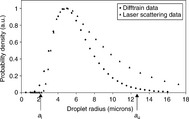
Fig. 6.11 Silicone oil emulsion droplet size distributions as measured by Difftrain and laser scattering measurements. The distribution is number-based, that is, any droplet size population reflects the corresponding number of droplets in the emulsion Reproduced with kind permission from Ref. 46; © Elsevier.
6.7 NMR spin relaxation
The Carr–Purcell–Meiboom–Gill (CPMG) sequence was introduced by Carr and Purcell47 and refined by Meiboom and Gill.48 During the experiment, a 90° pulse is first applied, and then followed by a series of 180° pulses with a time interval of τ (Fig. 6.12). The 180° pulses refocus the processing spins and then the “echoes” can be obtained at the time 2nτ (n = 1, 2, 3, …). The decay curve of the CPMG signal is related to the spin–spin relaxation time T2. A CPMG experiment is analyzed by Equation 6.16 as follows.
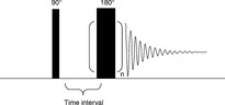
Fig. 6.12 Sequences of the pulses and the echoes in a CPMG experiment, the related parameters are also shown.
Bi is the signal intensity related to component i; T2,i is the spin–spin relaxation times of component i.
6.7.1 Determination of binding between proteins and polysaccharides
NMR water proton relaxation measurement, which is based on studying water molecule mobility in biopolymer solutions, has been used to characterize the structure of plant proteins and plant protein–polysaccharide mixtures in aqueous solutions.49 Figure 6.13 displays T2 measurement of protein, polysaccharide and protein–polysaccharide mixture solutions. The spin–spin relaxation time (T2) in the pea globulin solution at pH 2.75 was ~ 15% higher than that in the solution at pH 3.5 and 4 (Fig. 6.13 a)49 at 283 K. T2 remained at a relatively high value at lower pH values over the entire temperature range, indicating that water molecules had longer free paths at pH 2.75 and structural conformation greatly changed between pH 2.75 and 3.5. At pH 2.75, the intrinsic viscosity of the solution is low so the protein conformation is less compact.
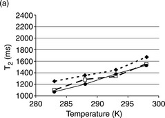
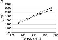
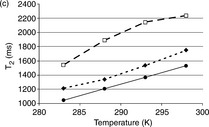
Fig. 6.13 T2 measurements as a function oftemperature in the range 283–298 K. The effect of pH is shown for various macromolecules and their mixtures. The total polymer concentration is 5 g/L.(< img >) : standard deviation. (--![]() --) pH 2.75, (-
--) pH 2.75, (-![]() -) pH 3.5, (-
-) pH 3.5, (-![]() -) pH 4. (a) Pea globulin; (b) Gum arabic; (c) Pea globulin/gum arabic mixtures with a ratio of 1:1 Reproduced with kind permission from Ref. 49; © Elsevier.
-) pH 4. (a) Pea globulin; (b) Gum arabic; (c) Pea globulin/gum arabic mixtures with a ratio of 1:1 Reproduced with kind permission from Ref. 49; © Elsevier.
In gum arabic solutions (Fig. 6.13b),49 the mobility increase with temperature was more significant. Simultaneous linear increases were observed. However, the effect of pH on gum arabic was less pronounced than on pea proteins. In all the conditions studied, T2 values from gum arabic solution were significantly higher than those obtained from pea protein solutions. This behavior could be related to the structural differences between proteins and polysaccharides. Gum arabic solutions display low viscosity, and gum arabic forms random coils with small hydrodynamic radii, features which are consistent with the higher T2 values.
To investigate water mobility in protein/polysaccharide mixtures (Fig. 6.13c),49 the protein/polysaccharide weight ratio was kept constant (1:1). The optimal pH condition for (1:1) pea globulin/gum arabic coacervation observed was pH 3.5 and this was in agreement with data in previous literature. At pH 3.5, pea globulin and gum arabic formed well-dispersed coacervate particles. In the NMR spin–spin relaxation study, the T2 values at pH 3–3.5 were significantly higher than those under other pH conditions over the whole temperature range studied. Meanwhile, the T2 values of protein/polysaccharide mixtures obtained at this pH region were also higher than those obtained from individual protein or polysaccharide solutions. High water mobility at pH 3.5 caused phase separation. The protein/polysaccharide mixtures were phase-separated, forming a concentrated coacervate phase and a polymerdepleted supernatant with many free water molecules. The temperature effect was markedly significant in the range of 283–293 K, indicating that hydrophobic interaction and hydrogen bonding may occur. The hydrogen bonding was attenuated by higher temperatures in the second range (temperatures beyond 293 K), which was verified by T2 value plateau. The T2 values of two other mixtures obtained at pH 2.75 and pH 4 were similar to those obtained for the pea globulin solution alone.
6.8 Time domain (TD)-NMR technique
The FID signal detected after one 90° pulse is the simplest relaxation signal which flips the equilibrium magnetization M0 onto the XY plane as shown in Fig. 6.14.50 After the 90° pulse, the magnetic moments greatly lose rotational coherence due to the energy exchanges and magnetic field inhomogeneities. The signal is detected when there is a decrease of the transverse magnetization vector in dispersion. This process is quicker for the protons in solid phase than the protons in liquid phase.
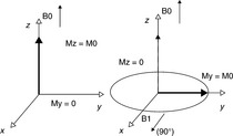
Fig. 6.14 Effect of a radio frequency pulse on the equilibrium magnetization Reproduced with kind permission from Ref. 51; © Elsevier.
6.8.1 Water content determination
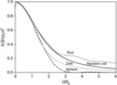
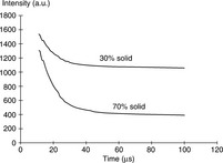
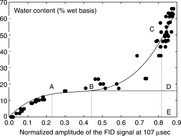
In TD-NMR, the relaxation of protons in more solid phases is faster than that of protons in more liquid phases. Therefore, it is possible to obtain information about the proportions of protons in these two phases. Figure 6.15 clearly shows that the signal from protons in solid phases decays very rapidly and the signal from protons in liquid phases decays relatively slowly.50 The proton proportion in those solid/ liquid mixture samples can be gained directly from the FID signal decay following a 90° RF pulse. It is also possible to use TD-NMR technique to obtain information about the proportions of bound and free water in food matrices. After extrapolating the SRC (slow relaxing components) signal back to 0 μs after the pulse, the amounts of bound water and free water can be obtained. Figure 6.16 displays the relationship between water content and intensity of SRC for gelatin.51 The amplitude of the FID signal went up when the water content increased. At point B, there is a clear inflexion. For gelatin, the inflexion point was located at 18.8% water, which is equivalent to 0.23 g water per gram dry gelatin, almost the same value as the amount of non-freezing water in gelatin obtained from the sorption isotherm.
6.9 Conclusions and future trends
This chapter introduces two advanced technologies – SAXS and NMR – and their applications for food materials characterizations. With the development of modern synchrotron X-ray facilities, SAXS has become a powerful technique for structural investigation, especially for materials of small molecular weight (i.e. short bioactive peptides) and low concentrations. NMR offers non-invasive and nondestructive methods for probing local structure and interactions in food ingredients such as proteins, polysaccharides and food emulsions. It is very important to establish structure–property relationship among multi-component food systems, as this helps food scientists to explore nanostructures more conveniently. In the future, it will be possible to apply these two techniques to understand factors affecting the nutritional value, texture and taste of foods at the molecular level and to combine the fundamentals of nanotechnology and polymer/colloid chemistry with food science to invent and develop novel food products with improved functionality, palatability and safety.
6.11 References
1. Mezzenga, R., schurtenberger, P., Burbidge, A., Michel, M. Understanding foods as soft materials. Nature Materials. 2005; 4:729–740.
2. Coppens, P., Penner-Hahn, j. Introduction: X-rays in chemistry. Chemical Reviews. 2001; 6:1567–1568.
3. Beaucage, G., rane, S., Sukumaran, S., Satkowski, M.M., Schechtman, L.A., Doi, Y. Persistence length of isotactic poly(hydroxy butyrate. Macromolecules. 1997; 30:4158–4162.
4. Bras, W., Ryan, A.J. Sample environments and techniques combined with small angle X-ray scattering. Advances in Colloid & Interface Science. 1998; 75:1–43.
5. Svergun, D.I., Koch, M.H.J. Small-angle scattering studies ofbiological macromolecules in solution. Report on Progress in Physics. 2003; 66:1735–1782.
6. Roe, R.J. Methods of X-Ray and Neutron Scattering in Polymer Science. New York: Oxford University Press; 2000.
7. Debye, P. Zerstreuung Von Röntgenstrahlen. Annalen der Physik. 1915; 46:809.
8. Larue, K., Adam, M., Da Silva, M., Sheiko, S.S., Rubinstein, M. Wormlike micelles of block copolymers: Measuring the linear density by AFM and light scattering. Macromolecules. 2004; 37(13):5002–5005.
9. Yunqi, L. Investigation of physical gelation in polymer solutions using a combination of Monte Carlo simulation and small-angle neutron scattering, PhD dissertation, Chang Chun Institute of Applied Chemistry, 2006. [Chinese Academy of Science].
10. Kroy, K., Frey, E. Dynamic scattering from solutions of semiflexible polymers. Physical Review E. 1997; 55:3092–3101.
11. Guinier, A., Fournet, G. Small-Angle Scattering of X-rays. New York: John Wiley and Sons; 1955.
12. Lipfert, J., Columbus, L., Chu, V.B., Lesley, S.A., Doniach, S. Size and shape of detergent micelles determined by small-angle X-ray scattering. Journal of Physical Chemistry B. 2007; 111:12427–12438.
13. Kratky, O., Porod, G. Röntgenuntersuchung gelöster Fadenmoleküle. Receuil des Travaux Chimiques. 1949; 68:1106–1122.
14. Portnaya, I., Ben-Shoshan, E., Cogan, U., Khalfin, R., Fass, D., Ramon, O., Danino, D. Self-assembly of bovine beta-casein below the isoelectric pH. Journal of Agricultural and Food Chemistry. 2008; 56:2192–2198.
15. Glatter, O. A new method for the evaluation of small-angle scattering data. Journal of Applied Crystallography. 1977; 10:415–421.
16. Moore, P.B. Small-angle scattering: Information content and error analysis. Journal of Applied Crystallography. 1980; 13:168–175.
17. Provencher, S.W. Contin: A general purpose constrained regularization program for inverting noisy linear algebraic and integral equations. Computer Physics Communications. 1982; 27:213–227. [229–242].
18. Semenyuk, A.V., Svergun, d.i. GNOM – a program package for small-angle scattering data processing. Journal of Applied Crystallography. 1991; 24:537–540.
19. Svergun, D.I. Determination of the regularization parameter in indirect-transform methods using perceptual criteria. Journal of Applied Crystallography. 1992; 25:495–503.
20. Ilavsky, J., Jemian, P.R. Irena: Tool suite for modeling and analysis of small-angle scattering. Journal of Applied Crystallography. 2009; 42:347–353.
21. Hong, X.G., Hao, Q. High resolution pair-distance distribution function P(r) of protein solutions. Applied Physics Letters. 2009; 94:083903.
22. Hailong, Y., Qingrong, H. Enhanced in vitro anti-cancer activity of curcumin encapsulated in hydrophobically modified starch. Food Chemistry. 2010; 119:669–674.
23. Rieker, T., Hanprasopwattana, A., Datye, A., Hubbard, P. Particle size distribution inferred from small-angle X-ray scattering and transmission electron microscopy. Langmuir. 1999; 15:638–641.
24. Spagnuolo, P.A., Dalgleish, D.G., Goff, H.D., Morris, E.R. Kappa-carrageenan interactions in systems containing casein micelles and polysaccharide stabilizers. Food Hydrocolloids. 2005; 19:371–377.
25. Hura, G.L., Menon, A.L., Hammel, M., Rambo, R.P., Poole, F.L., Tsutakawa, S.E., Jenney, F.E., Classen, S., Frankel, K.A., Hopkins, R.C., Yang, S.J., Scott, J.W., Dillard, B.D., Adams, M.W.W., Tainer, J.A. Robust, high-throughput solution structural analyses by small angle X-ray scattering (SAXS). Nature Methods. 2009; 6:606–612.
26. Shamai, K., Shimoni, E., Bianco-Peled, H. Small angle X-ray scattering of resistant starch type III. Biomacromolecules. 2004; 5:219–223.
27. Pitkowski, A., Nicolai, T., Durand, D. Scattering and turbidity study of the dissociation of casein by calcium chelation. Biomacromolecules. 2008; 9:369–375.
28. Forato, L.A., Doriguetto, A.C., Fischer, H., Mascarenhas, Y.P., Craievich, A.F., Colnago, L.A. Conformation of the Z19 prolamin by FTIR, NMR, and SAXS. Journal of Agricultural and Food Chemistry. 2004; 52:2382–2385.
29. Jin, K.S., Rho, Y., Kim, J., Kim, H., Kim, I.J., Ree, M. Synchrotron small-angle X-ray scattering studies of the structure of porcine pepsin under various pH conditions. Journal of Physical Chemistry B. 2008; 112:15821–15827.
30. Akiba, I., Terada, N., Hashida, S., Sakurai, K. Encapsulation of a hydrophobic drug into a polymer-micelle core explored with synchrotron SAXS. Langmuir. 2010; 26:7544–7551.
31. Shrestha, L.K., Glatter, O., Aramaki, K. Structure of nonionic surfactant (glycerol alpha-monomyristate) micelles in organic solvents: A SAXS study. Journal of Physical Chemistry B. 2009; 113:6290–6298.
32. Huang, Y.P., Yu, H.L., Guo, L., Huang, Q.R. Structure and self-assembly properties of a new chitosan-based amphiphile. Journal of Physical Chemistry B. 2010; 114:7719–7726.
33. Pedersen, J.S., Gerstenberg, M.C. Scattering form factor of block copolymer micelles. Macromolecules. 1996; 29:1363.
34. Pascal, C., Legrand, C.P., Imberty, A., Gautier, C., Manchado, P.S., Cheynier, V., Vernhet, A. Interactions between a non glycosylated human proline-rich protein and flavan-3-ols are affected by protein concentration and polyphenol/protein ratio. Journal of Agricultural and Food Chemistry. 2007; 55:4895–4901.
35. Jobstl, E., O’Connell, J., Fairclough, J.P.A., Williamson, M.P. Molecular model for astringency produced by polyphenol/protein interactions. Biomacromolecules. 2004; 5:942–949.
36. Pascal, C., Legrand, C.P., Cabane, B., Vernhet, A. Aggregationofaproline-rich protein induced by epigallocatechin gallate and condensed tannins: Effect of protein glycosylation. Journal of Agricultural and Food Chemistry. 2008; 56:6724–6732.
37. Sokolova, A., Kealley, C.S., Hanley, T., Rekas, A., Gilbert, E.P. Small-angle X-ray scattering study of the effect of pH and salts on 11S soy glycinin in the freeze-dried powder and solution states. Journal of Agricultural and Food Chemistry. 2010; 58:967–974.
38. Ma, X., He, P.L., Sun, P., Han, P. Lipoic acid: An immunomodulator that attenuates glycinin-induced anaphylactic reactions in a rat model. Journal of Agricultural and Food Chemistry. 2010; 58:5086–5092.
39. Garasanin, T., Cosgrove, T., Marteaux, L., Kretschmer, A., Goodwin, A. NMR self-diffusion studies on PDMS oil-in-water emulsion. Langmuir. 2002; 18:10298–10304.
40. Murday, J.S., Cotts, R.M. Self-diffusion coefficient of liquid lithium. Journal of Chemical Physics. 1968; 48:4938–4945.
41. Douglass, D.C., Mccall, D.W. Diffusion in paraffin hydrocarbons. Journal of Physical Chemistry. 1958; 62:1102–1107.
42. Johansson, L., Elvingson, C., Skantze, U., Lofroth, J.E. Diffusion and interaction in gels and solutions. Progress in Colloid and Polymer Science. 1992; 89:25–29.
43. Garti, N., Spernath, A., Aserin, A., Lutz, R. Nano-sized self-assemblies of non-ionic surfactants as solubilization reservoirs and microreactors for food systems. Soft Matter. 2005; 1:206–218.
44. Buckley, C., Hollingsworth, K.G., Sederman, A.J., Holland, D.J., Johns, M.L., Gladden, L.F. Applications of fast diffusion measurement using Difftrain. Journal of Magnetic Resonance. 2003; 161:112–117.
45. Stamp, J.P., Ottink, B., Visser, J.M., Van DuynhoVen, J.P.M., Hulst, R. Difftrain: A novel approach to a true spectroscopic single-scan diffusion measurement. Journal of Magnetic Resonance. 2001; 151:28–31.
46. Hollingsworth, K.G., Sederman, A.J., Buckley, C., Gladden, L.F., Johns, M.L. Fast emulsion droplet sizing using NMR self-diffusion measurements. Journal of Colloid and Interface Science. 2004; 274:244–250.
47. Carr, H.Y., Purcell, E.M. Effects of diffusion on free precession in nuclear magnetic resonance experiments. Physical Review. 1954; 94:630–638.
48. Meiboom, S., GILL, D. Modified spin-echo method for measuring nuclear relaxation times. Review of Scientific Instruments. 1958; 29:688–691.
49. Ducel, V., Pouliquen, D., Richard, J., Boury, F. 1H NMR relaxation studies of protein-polysaccharide mixtures. International Journal of Biological Macromolecules. 2008; 43:359–366.
50. Rutledge, D.N. Characterization of water in agro-food products by time domain-NMR. Food Control. 2001; 12:437–445.
51. Vachier, M.C., Rutledge, D.N. Hydration state of gelatin studied by time domain nuclear magnetic resonance (TD-NMR): A preliminary study. Food Chemistry. 1996; 57:287–293.