12
Process Safety in Natural Gas Industries
Monir Ahammad and M. Sam Mannan
Mary Kay O'Connor Process Safety Center, Artie McFerrin Department of Chemical Engineering, Texas A&M University, USA
Chapter Menu
- Introduction
- Incident History
- Process Safety Methods
- Equipment and Plant Reliability
- Facility Siting and Layout Optimization
- Relief System Design
- Toxic and Heavy Gas Dispersion
- Fire and Explosion
- Effective Mitigation System
- Regulatory Program and Management Systems for Process Safety and Risks
- Concluding Remarks
Introduction
Natural gas streams may contain H2S and organic volatiles (i.e., mercaptans) that have toxic health effects. Refrigerants (e.g., ammonia and propane are often used for lowering process temperature in LNG facilities) can also have both toxic and flammable effects when released to the environment. The American Industrial Hygiene Association (AIHA) has issued Emergency Response and Guidelines (ERPGs) for air contaminants such as H2S, NH3 and methyl‐mercaptans. An exposure of H2S at a concentration level of 100ppm up to an hour is considered as life threatening for human beings. Process Safety is the science, technology, and management system to prevent, and mitigate unwanted events such as exposure of H2S.
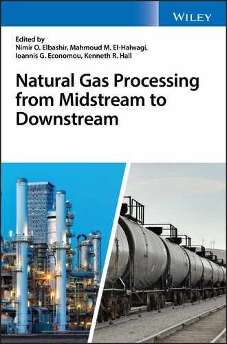
The application of process safety principles begins with the identification of hazards. A hazard can be a material, or an activity, or a procedure that can cause harm to human, or environment, or incur economical loss. For example, a large release of liquefied natural gas (LNG) may create an asphyxiating environment. LNG being stored at −162°C, its vapor is heavier than air, and therefore an unignited vapor cloud resulting from a loss‐of‐containment event may engulf a large area, causing an asphyxiating environment. An ignition of such flammable vapor cloud may lead to a flash fire returning to the source of the leak. Depending on the congestion or confinement level in the facility, a delayed ignition can cause deflagration to mild vapor cloud explosion. This scenario would be completely different if the released flammable material is propane or other refrigerants with detonating characteristics. A propane vapor cloud explosion may result in detonation and can severely damage the facility. Figure 12.1 depicts different hazards associated with natural gas industries. An immediate ignition of pressurized flammable gas/liquid leak would result in a jet fire. Flashfire occurs during a delayed ignition of flammable vapor mixed with air. Fire burning a liquid pool, whether spreading or fixed diameter, are referred as pool fire.
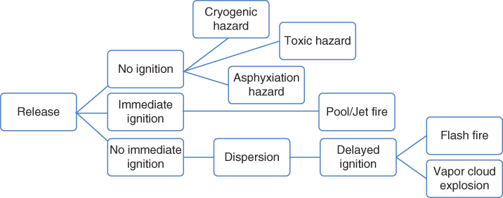
Figure 12.1 Hazards related to natural gas processing.
Incident History
Process safety incidents are prevalent in all types of industries including natural gas. Hirschberg et al. (2004) analyzed ENSAD (Energy‐related Severe Accident Database), established by the Paul Scherrer Institute (PSI), for a comparative perspective on severe incidents in the energy sector. The study separates LPG from natural gas. Figure 12.2(a) shows a comparison of an aggregated normalized number of affected people per gigawatt (GW) of energy production among different industries. There is no significant difference between the personal injuries among the countries worldwide. The study shows that among the energy sectors, LPG has the largest damage indicator and nuclear power is the lowest. Though the natural gas industry lies in a moderate region based on the statistics, in the LNG liquefaction process, propane and butane are separated from the natural gas stream, an accidental leak from those streams has the damage potential as high as LPG production. Figure 12.2(b) shows the societal risk curve for different energy sectors in the OECD countries. Among the fossil energy chains, the natural gas industry has the lowest frequency of severe incidents involving fatalities, whereas LPG has the highest frequency of fatality. Despite favorable statistics, incidents in natural gas industries keep happening. Some well‐publicized disasters related to natural gas processing and transportation are discussed below.
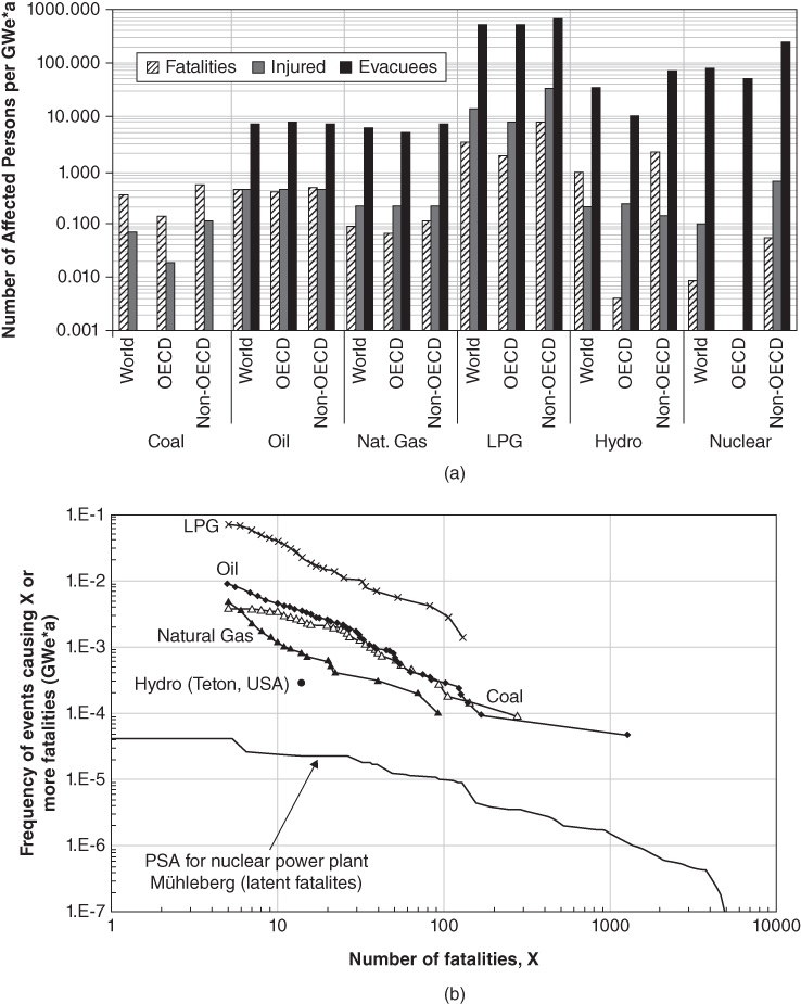
Figure 12.2 (a) Comparison of energy‐related damage rates occurred worldwide in the period of 1969‐1996; (b) Frequency – Consequence (F‐N) curve for severe incidents in various energy chains in OECD countries during 1969‐1996.
Reprinted from Journal of Hazardous Materials, Vol 111, Stefan Hirschberg, Peter Burgherr, Gerard Spiekerman, and Roberto Dones, Severe accidents in the energy sector : comparative perspective, pp. 57‐65, Copyright (2004), with permission from Elsevier.
Figure 12.3Figure 12.3Destruction after San Bruno incident, 2010 (Source: Wikipedia).
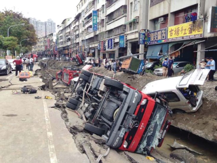
Figure 12.4Figure 12.4Havoc caused by the Kaohsiung gas explosion, Taiwan, 2014. Reprinted with permission from Process Safety Progress, Vol 35, Issue 3, Horng‐Jang Liaw, Lessons in process safety management learned in the Kaohsiung gas explosion accident in Taiwan: 228‐232, Copyright (2016) John Wiley & Sons.
Cleveland, Ohio, 1944
On October 20, 1944, LNG storage tank number four collapsed catastrophically due to the brittle fracture of the tank wall. The released content flowed into the streets and sewers due to the absence of secondary containment (e.g., dike). The resulting vapor cloud ignited, causing explosions and fires. Jets of fire erupted from the manholes of sewers, and the manhole covers were thrown miles away. The fire caused significant structural damage to a nearby spherical LNG storage tank because it had no insulation against fire. Once the fire was extinguished, people started returning to their homes and businesses thinking that the matter has been taken care of. A second release occurred from the damaged tank of an additional 15,000 kg of LNG. The explosions and fire resulting from the ignition of the evaporating LNG continued to occur engulfing homes and traveling through sewers. The incident killed at least 200 people and caused extensive property damage. Improper choice of tank material (3.5% Ni‐ Steel) led to a low‐temperature embrittlement, which was exacerbated by vibrations from the nearby railroad.
Skikda, Algeria, 2004
On January 19, 2004, an explosion at the Sonatrach liquefaction facility resulted in 27 fatalities, 72 injuries, and destruction of 3 LNG manufacturing trains, a marine berth, 76% down production, and $900 million in total losses. At 6:39 PM, an operator noticed a pressure rise in the steam boiler 40 unit, opening safety relief valves. Despite reducing the pressure of the fuel gas flow to the burner to a minimum setting, the operator was not able to reduce the pressure. After one minute, the operator from the nearby liquefaction train 30 informed the train 40 operator via intercom that a vapor cloud was forming. At the same time, an explosion was heard following another immediate explosion and a huge fireball. The ensuing fire and explosions totally destroyed liquefaction trains 40, 30, and 20.
The incident occurred due to the leakage of refrigerant (cold hydrocarbon) near the boiler of liquefaction train 40. The uncontrolled gas entrance in the boiler formed an explosive mixture, which eventually exploded, destroying the boiler and igniting the vapor cloud formed outside. Investigations found that the facility siting and layout optimization, control of ignition sources, and appropriate placement of gas detectors could have reduced the damage (Dweck et al. 2004).
San Bruno, California, 2010
On September 10, 2010, the natural gas transmission pipeline operated by Pacific Gas and Electric Company (PG&E) ruptured. The subsequent underground explosion caused 8 fatalities, multiple injuries, destruction of 38 homes, and damage to additional 70 houses (Richards 2013). The ruptured pipeline had a 30‐inch diameter at an operating pressure of 400 psig. The U.S. National Transportation Safety Board (NTSB) reported that a big piece of steel pipe was blown about hundred feet away producing a 72‐foot crater. It is also reported that the mechanical integrity of a piece of pipe section was lost due to improper welding. The released gas from the leak accumulated in the underground airspace around the pipeline and formed a flammable gas‐air mixture, which ultimately found the ignition source (Peekema 2013).
Kaohsiung, Taiwan, 2014
On July 31, 2014, a series of underground gas explosions due to the leak of propylene killed 32 persons and injured another 321. The blast destroyed 6 km of roads, overturned and trapped cars and fire trucks. The pipeline operated by China General Terminal and Distribution (CGTD) was delivering propylene to the LYC Chemical Corporation. Investigations found that following an observation of abnormal pressure in a 4‐inch pipeline, the gas transmission was shut down after 2 hours. Meanwhile, an estimated amount of 20 tons of propylene was released. The leak seeped into the sewer system and found an ignition source. The leak was the result of corrosion in the presence of moisture (Liaw 2016).
Process Safety Methods
The principles of process safety ensure the design intent of equipment, unit, plant, procedure, and management systems are satisfied during all the stages of the project. Loss of containment of hazardous materials, unplanned energy release, and unplanned human activity may lead to unwanted consequences. Therefore, process safety methods seek to identify associated hazards and risks in order to develop appropriate measures for implementing, measuring, evaluating, and monitoring safety. Figure 12.5 graphically categorizes existing process safety methods according to their purposes. The methods are classified into five groups, namely methods to (1) identify process hazards, (2) implement safety, (3) measure process safety, (4) evaluate process safety, and (5) monitor process safety performance. As shown in the figure, the knowledge of process design, management, and systems such as monitoring, inspection, control, mitigations, safety barriers, and operating procedures are needed for the effective use of process safety methods.
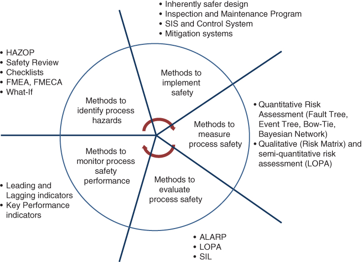
Figure 12.5 Process safety methods and their purpose.
The methods to identify process hazards are intended to link relationships between the hazards, causes, and the potential consequences. Hazard and Operability (HAZOP) Study, Safety Review, Checklists, Failure Mode and Effect Analysis (FEMA), Failure Mode, Effect and Criticality Analysis (FMECA) and What‐If are used frequently. HAZOP, a structured method that is most used, starts with identifying a node; the keywords are used to understand the potential consequences of deviation from the design intent for that node. However, it is not suitable for identification of mechanical integrity failures and external events (Khan and Hashemi 2017). The safety review is a less rigorous study than HAZOP and intends to find initiating events that can cause incidents. It also reviews previous incidents and recommends safety measures (Crowl and Louvar 2011). Often checklists are used to identify process hazards due to ease of implementation. The effectiveness of checklist methods depends on the quality of checklists and personal experiences. The What‐If method asks “what‐if” questions of potential deviations from design intents for the cause and consequence relationships. As the name suggests, FMEA and FMECA are very structured methods, applied to critical and complex equipment at the component level, to identify the cause and effect of component failure.
After identification of the causes and consequences of potential incidents, safety measures also known as control measures or barriers need to be implemented to prevent the incident from occurring. The barrier strategy can be classified into three categories. Inherently Safer Design is the first category, which is highly effective and uses the principle of elimination, substitution, minimization, and moderation of hazards. Engineering barriers, also recategorized as passive and active barriers, are the second choice in implementing safety barriers. Passive barriers do not require any human interventions, and therefore the effectiveness of preventing an incident is much higher, e.g., dikes, firewalls, gravity drains, flame arrestors. Control systems, shut‐down systems, and relief devices are considered active barriers. Finally, administrative barriers such as rules, standard operating procedures, and training are considered in implementing safety.
The risk is used as a measure of safety, which is defined as the combination of the probability of a certain scenario combined with a certain consequence. Existing risk assessment methods can be classified as: a) quantitative—e.g., Event Trees, Fault Trees, Bow‐tie, Bayesian Network; b) semiquantitative—e.g., Layer of Protection Analysis (LOPA); and c) qualitative—e.g., Risk Matrix. In quantitative risk assessment (QRA), both the probability of the incident and the associated consequences are estimated quantitatively. In semiquantitative risk assessment, usually the probability estimation is quantitative, and the consequence is determined qualitatively. Both the probability and the consequences are estimated qualitatively for a qualitative risk assessment, and acceptability of risk is determined by comparing to a risk matrix. The assessed risk is evaluated to choose whether it is acceptable for the plant personnel, public, or environmental damage. There are no universal criteria for evaluating risk. Existing practice includes a demonstration that the adopted barriers reduce risk to a level called As‐Low‐As‐Reasonably‐Practicable (ALARP). In LOPA, the criteria of acceptable risk are defined based on the company's tolerable risk criteria. Safety Integrity Level (SIL) target assessment further studies the risk reduction credited for the implementations of safety instrumented functions (SIF).
The health of safety systems is monitored using leading and lagging indicators. Use of leading indicators provides a proactive measure in preventing incidents or deteriorating conditions by detecting early signs. On the other side of the process safety spectrum, lagging indicators measure performance based on fatality, injury, first aid, and the number of releases and therefore are not effective in prevention and mitigation of incidents. Figure 12.6 illustrates lagging and leading indicators on the same scale. Most of the downstream oil and gas industries have adopted API RP 754 (API 2010) for safety indicators, but recent advancements propose risk‐based performance indicators (Khan et al. 2009).
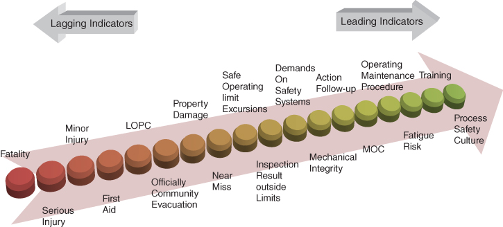
Figure 12.6 Leading and lagging indicators to measure safety performance. Reprinted with permission from Process Safety Progress, Vol 32, Issue 4, Wang., M., Mentzer, R.A., Gao, X., Richardson, J., & Mannan, M.S., Normalization of the process safety lagging metrics: 337‐345, Copyright (2013) John Wiley & Sons.
Equipment and Plant Reliability
Among many reasons, one major reason for incident occurrence is a failure of equipment. Equipment can fail instantly or over a long period of time due to its use. When a piece of equipment fails to perform its intended design purpose, it leads to unwanted consequences. The functionality of a system (e.g., level control loop) depends on the performance of the individual components (e.g., sensors, valves, logic controller, and wiring). Failure characteristics of these components determine the functionality of the overall system.
The reliability of a plant is determined based on probabilistic analysis of the failure of systems to minimize the cost of system downtime, spares, repair equipment, personnel, and warranty claims. It is an important factor in designing engineering systems to perform satisfactorily throughout their life cycle. The high reliability of a plant often also indicates higher safety factors. It ensures that individual pieces of equipment are reliable enough to ensure a safer processing plant. Thus, probabilistic assessments of the individual elements are performed to establish plant reliability. Reliability analysis is also the basis of other safety studies such risk assessment, failure mode analysis, and ensuring the Safety Integrity Level (SIL) of Independent Protection Layers (IPL). If the existing safety barriers do not mitigate the risk to a tolerable limit, a higher reliable system is often recommended during the hazard analysis stage. Such systems need verifications to ensure the validity of risk reduction measures and therefore reliability analysis is conducted.
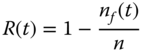
The definition of reliability implies that if after t period of operation, n f number of pieces of equipment out of n failed, then reliability of the equipment is given by,
The failure rate is a function of the quantity of the equipment, also called “failure density function,” is expressed as,
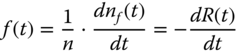
After a time t, of testing period, we know how many pieces of the equipment survived. Therefore, the conditional instantaneous failure rate, commonly known as hazard rate, becomes a very useful parameter, and it is defined as,
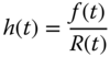
Figure 12.7 refers to the general behavior of equipment. The failure rate is high during the commissioning of the equipment, due to factors such as defective equipment, incorrect installations, substandard parts and materials, poor quality control, start‐up human error, inadequate debugging, incorrect packaging, inadequate process, and poor handling methods. It is also known as the burn‐in region in the bathtub curve. During the useful life region, a constant failure rate can be caused by the random fluctuations of the equipment operations. It may result from undetected defects, abuse, low safety factors, higher random stress, unavoidable conditions, and human error. If equipment consists of many pieces with different failure distributions, the overall effect may also result in a constant failure rate. This is the longest period of the equipment life, for which h(t) = λ, gives –
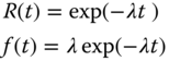
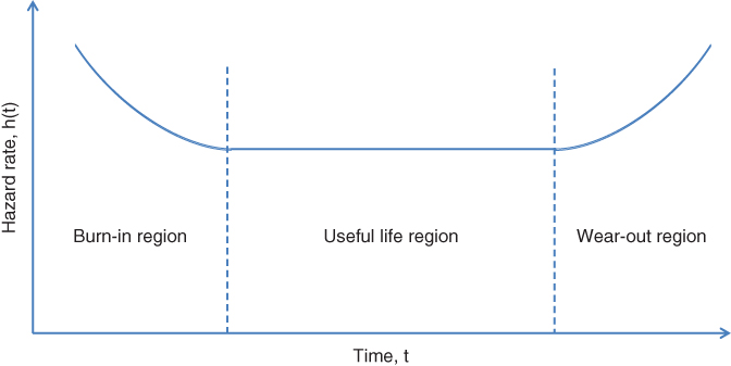
Figure 12.7 Bathtub curve for hazard rate.
The equipment wears out at the end of its life increasing its failure rate. Contributing reasons are poor maintenance, friction, aging, corrosion and creep, wrong overhaul, and short design‐in life.
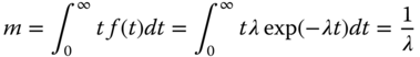
The mean life of equipment, also known as mean time to failure (MTTF) or mean time between failure (MTBF), can be calculated as:
For a system consisting of n components in series, the reliability of the whole system can be expressed in terms of individual components reliability as follows:

Thus, the failure rate of the system is

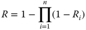
A parallel system fails only if all components fail simultaneously. Thus, the reliability and MTTF of such systems are:
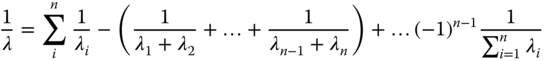
The reliability of a bridge network of components as shown in Figure 12.8 is expressed as follows:

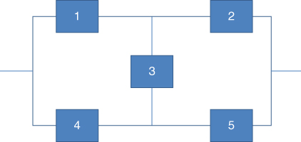
Figure 12.8 Bridge network of components.
A system where n components are in parallel operation but r components are functional, binomial distributions can be applied to determine the failure rate of such system. In a system with redundant components, where one component is operating and others are standby, it can be assumed that the standby component has zero failure rates. A Poisson distribution can be used for estimating the reliability of such a system.
There are many reliability evaluation techniques available. The most commonly used methods are:
- • Network Reduction Method
- • Fault Tree Analysis (FTA)
- • Markov Method
- • Decomposition Method
- • Failure Mode and Effects Analysis (FMEA)
The network reduction method simply evaluates the system reliability, as it is composed of independent series and parallel subsystems. A bridge configuration can be converted to equivalent series and parallel system using delta‐Y conversion.
Fault tree analysis (FTA) is very popular for reliability analysis and identifying the hazardous pathways leading to incidents. Modern FTA can be very large and complex, and thus computer software is often used. It is basically based on “AND” and “OR” logic operations. For example, in Figure 12.9, a heat exchanger overpressurization can occur due to the failure of alarm and failure to initiate emergency shutdown system. Each of these items can further be analyzed for the causes. Thus, there are four ways in which the over pressurization can occur. Each individual path is called cut‐sets. The probability of the top event is the summations of all cut‐sets. The minimum number of ways the event can occur is called “minimal cut‐sets.”
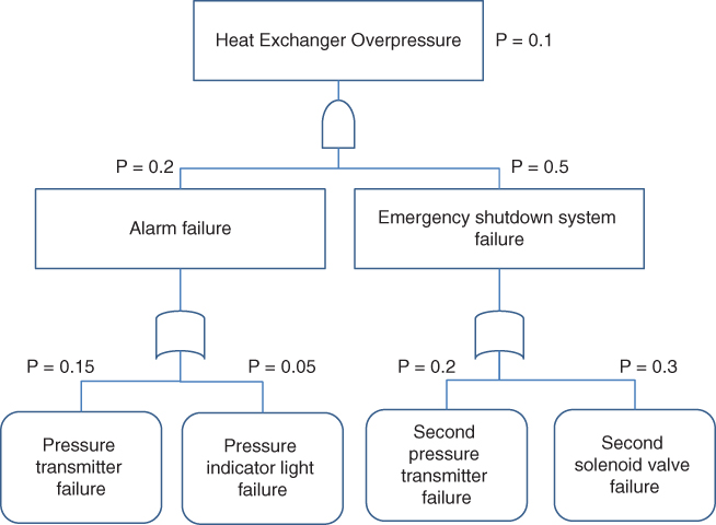
Figure 12.9 Example Fault Tree.
The Markov method assumes that the transition from a system state (e.g., operational) to another state (e.g., failed equipment) after a finite time interval Δt occurs at λ transition rate.
This gives,
The decomposition method simplifies a system into subsystems and applies conditional probability theory. The system probability can be measured by combining the subsystem probabilities. If A is a key element of a system S, which can have both a good state A, and a failed state, A ′, then the probability of the system failure can be determined by‐
FMEA is a step‐by‐step method to analyze all possible failure modes and their effect on the functionality of the system. Details on FMEA/FMECA can be found in (Dyadem Press., 2003).
Facility Siting and Layout Optimization
The primary consideration of facility siting is safety. Other factors that impact the siting of the natural gas processing plant and transportation system are sources of raw material, distance to market, access (e.g., raw materials, products, maintenance, operators, and emergency response), availability of land, sources of utility and effluent disposal, integrating with other plants, permits and regulatory policies, and investment incentives. Topography also becomes a crucial factor in the facility siting of the natural gas processing plant. As an example, during a loss of containment of LNG storage tank or a leak in a liquefaction process, heavy vapor (flammable or toxic) may flow towards a downhill, populated area and may cause catastrophic consequences such as Bhopal, 1984.
Separation distances between the hazards and potentially affected areas, within the plant boundary as well as to the public, can reduce the risk of the operation. This measure does not replace the importance of best practices in designing and operating a plant; however, it becomes a very effective measure as it is a passive protection layer in mitigating the consequences of major incidents. It is also an inherently safer strategy to separate the sources of potential fire, explosion, or toxic release from nearby populated areas. For example, a plant in a sparsely populated area will cause many fewer causalities compared to a plant in an urban area, in case of a major incident. Impacts on the surrounding area can be obtained from studies such as consequence analysis or hazard assessment. Facility siting improves safety in ways such as a) segregation of risks; b) limitation of exposure; c) mitigation of incident impacts; d) efficient and safe construction, operation, maintenance; e) better control room design; f) emergency control such as firefighting, access for emergency response; and g) security. Despite many advantages of large separation distances, plant economics determine the siting and optimum layout of the plant. Also, there are some disadvantages associated with large separation distances because additional space increases the costs in terms of land, pipework, and operating cost. Safety issues may also be impacted in terms of increased corrosion and maintenance requirements and greater opportunities for failure.
There are various ways of generating plant layout. A structured approach follows four stages. In the first stage, a 3D model is prepared to analyze the space and equipment placement based on operations access, maintenance access, and piping connections. In the second stage, the concept of “flow,” meaning the progression of process materials or utilities towards the final products or completion of the loop is applied to minimize the transfer of materials for economic reasons and minimizing potential release locations. In the third stage, the relationships between the items that share common factors, in the viewpoint of discipline, are identified. Example of relationships can be (1) process, (2) operational, (3) mechanical, (4) electrical, (5) structural, and (6) safety. In this stage, separation distances between equipment due to hazard consideration, fire and explosions, population density, and weather conditions, are applied. CCPS guidelines (CCPS 2003) provide a more detailed account of such relationships. In the fourth stage, the identified relationships are prioritized into groups to arrange items on the plot plan. A typical group should not include more than seven items. For example, a distillation column group should consist of the column itself and associated heat exchangers. The synthesized layout is then analyzed for
- Classification, rating, and ranking
- Critical examination
- Hazard assessment
- Consequence modeling
- Economic optimization
The plant layout is classified into areas such as fire hazard area, storage, firefighting facilities, access, and electrical area classification. In most cases, the quantity of material in storage, e.g., LNG, is much greater than the amount in the process. Storage classification is needed to meet safety requirements such as diking and venting. Storage sites are segregated from the process, in an open location to allow dispersion, diked to contain 110% of the total stored volume and designed to withstand heavy loads. Flammable liquid storage area classifications include: (1) liquid at atmospheric conditions, (2) pressurized storage, (3) refrigerated storage, and (4) gas under pressure. The electrical area classification is aimed to isolate ignition sources from flammable or combustible leaks and identifying potential safeguards to prevent fire. The International Electro‐Technical Commission (IEC) classifies process hazardous area into four categories: (1) zone 0: presence of flammable atmosphere for long periods; (2) zone 1: flammable atmosphere of short periods in normal operation; (3) zone 2: flammable atmosphere is not likely in normal operations but may occur for a short time; and (4) non‐hazardous area. In the USA, hazardous areas are classified as: (1) Class I: combustible material is gas or vapor; (2) Class II: combustible material is dust; and (3) Class III: combustible material is fiber in suspended form. Each class is subdivided into two divisions for distinctions between the frequencies of the substance presence in the atmosphere.
In the critical examination of a plant layout, the following questions are asked: Where is the plant equipment placed? Why is it placed there? Where else could it go? The alternatives are considered and critically examined for the best possible plant layout. Hazard assessment and consequence analysis are conducted to determine the risk in terms of the whole site, the effect on the occupied buildings due to leak, fire, vapor cloud explosion, and escalation of other scenarios. For more detail of the hazard assessment and consequence analysis please refer to Mannan (2012). Economic analysis of the alternative layouts is performed for decision making and determining the factors in terms of the cost of the plant layout, such as foundations, structures, piping and pipe tracks, pumps, and power consumptions.
The facility siting and plant layout activities can be broadly categorized as site layout, plot layout, and equipment layout, which undergo three stages: stage one layout, stage two layout, and final layout. In the stage one layout, significant consideration is given to items that may threaten project viability. Plots are generally considered as 100m X 200 m separated by 15m wide roads. Once the stage one preliminary plot layout is completed, it is then subjected to hazard assessments of smaller and frequent leaks with possible sources of ignition. For stage one site layout, separation distances, access requirements, traffic characteristics, material and utilities flow to the site are considered. Hazard assessment of site layout is performed to consider the escalation of incidents and vulnerability of service buildings both inside and outside of the boundary.
Figure 12.10 depicts the details of stage two and the final stage of plot and site layout in contrast with other process design activities. In stage two site layouts, reworking is done on stage one layout for the specific site, hazard assessment, economic optimization, and critical analysis. Legal requirements such as soil and drainage, meteorological conditions, environmental aspects, insurance, and emergency services are incorporated in this stage. International and national standards, company standards, contractor standards are considered in evaluating the process engineering design data: e.g., flow sheets, equipment drawings, pipeline lists. Table 12.1 summarizes the details of site layout and equipment layout considerations.
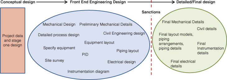
Figure 12.10 Stages of facility siting and plant layout.
Table 12.1 Site layout and plot layout considerations.
| Site Layout Features | Plot Layout Considerations |
|
|
Many factors determine the layout of equipment, e.g., usage of common facilities. Stacks, for disposal of gaseous and liquid effluents, might be common to different furnaces and fired heaters. The transfer line minimization, avoidance of trenches or pits that may hold flammable liquid under the furnace area, proper ventilation, minimization of peepholes and observation doors are also very important factors. Connecting pipe between heat exchangers is kept at a minimum with the provisions of pipe lengths to allow stress relief and access for maintenance. Pumps handling hot liquids are separated from pumps handling flammable and volatile liquids or from compressors handling flammable gases. Open or closed design of pumps and compressor houses also plays a significant role in ensuring appropriate ventilation. Corrosive materials cause a significant number of incidents among various industries.
Almost all the world's natural gas is transferred through networks of pipelines; thus, siting of transmission pipelines by itself requires a detailed study. The general considerations of piping layout within a processing plant should be minimum for both economic and safety reasons. Cost of emergency isolation valves, manual valves, relief valves and bursting disks, liquid drains, and associated instruments may increase with the increase of pipe runs.
Separation Distances
The primary constraint of plant layout is the separation distances. Approaches in considering appropriate separation distances can be classified into three categories: a) use of industry standards, b) use of ranking methods, and c) estimation of separation distances based on engineering calculations for the case. More description of using codes and standards are given by CCPS (2003) and Mannan (2012). Lewis (1980) used the Mond Index to determine the separation distances based on two values of overall risk ratings (ORR), R1 and R2. The minimum separation distances recommended in the industry standards are not a good practice for new projects. Thus, he used the index‐based methodology to minimize the risk to personnel, minimize escalation, and ensure adequate access for emergency response, allowing flexibility in combining units of similar hazards potential. Table 12.2 indicates the separation distances based on using the Mond index between process units and storage units.
Table 12.2 Minimum separation distances between a storage unit and a processing unit using the Mond Index, synthesized from Mannan (2012).
| Overall risk rating R2 of process unit | |||||||
| Overall risk rating R2 of storage unit | mild | low | medium | high | very high | extreme | very extreme |
| Mild | 3 | 7 | 10 | 13 | 18 | 23 | 38 |
| Low | 6 | 9 | 12 | 17 | 23 | 30 | 50 |
| Moderate | 9 | 12 | 17 | 21 | 31 | 44 | 66 |
| High | 12 | 17 | 21 | 28 | 43 | 56 | 84 |
| Very high | 17 | 23 | 31 | 43 | 56 | 72 | 110 |
| Extreme | 23 | 30 | 44 | 56 | 72 | 97 | 145 |
| Very extreme | 38 | 50 | 66 | 84 | 110 | 145 | 197 |
Recent advancements in modeling the consequences of hazardous releases allow more accurate estimation of separation distances. Such approaches are often referred as hazard models. Area contours based on threshold limiting value (TLV) for toxic or asphyxiating gas release, thermal radiation from fires, and overpressures from explosions are used to determine the separation distances. Special consideration or modeling needs to be done for liquefied flammable gas such as LPG. Consisting primarily of propane, the flammable vapor from LPG releases can cause vapor cloud detonations.
Advances in Facility Siting and Layout Optimizations
A significant amount of research has been conducted in the last decade to address the current shortcomings in safety and improvement of the facility siting and layout optimization techniques. A study (Mannan, West, and Berwanger 2007) of several recent incidents and historical data (which includes: 1) the Texaco Refinery, Milford Haven Wales, 1994; 2) the Bellingham pipeline rupture, 1999; 3) the BP Texas City Refinery, 2005; 4) Terra industries, IA, 1994; 5) Tosco Martinez Refinery, CA, 1999; 6) Shell chemical, TX, 1997; and 7. Surpass Chemical, NY, 1997) draws attention to the fact that the probability and severity of catastrophic incidents can be greatly impacted by facility siting issues. Despite the fact that many of the studied industries are refineries and downstream chemical companies, the findings are prevalent in all industries including natural gas midstream to downstream operations. The weakness of regulations, standards, and management systems pertaining to facility siting were evaluated. For an effective facility siting management system, the authors recommended an easy‐to‐understand method, consideration of protection from vapor cloud explosions, shelter‐in‐place for toxic releases, and removal of temporary buildings before start‐up.
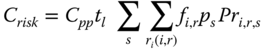
Vázquez‐Román et al. (2010) have presented a stochastic approach in determining the optimal facility layout by considering the effect of toxic release. The objective of their mathematical model is to minimize the cost of piping, land, and risk as expressed below.
where,
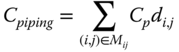
| C p | Cost of a pipe, $/m |
| d i, j = (x i − x j )2 + (y i − y j )2 | Center‐to‐center distance between two units, m |
| C l | Land cost per square meter, $/m2 |
|
|
Length of subunits in the x, y‐direction, m |
| f i, r | Frequency of the type of release, r, in unit i |
| P s | Expected population in the facility |
| C pp | Compensation cost per fatality |
| t l | Expected lifespan of the plant |
Constraints such as land, nonoverlapping of two units, minimum separation distances, and toxic release are used to simulate real facility siting issues. Weather conditions significantly affect the consequences of a toxic release; therefore, to evaluate the risk of such release, a stochastic model of weather conditions using wind speed, wind direction, and atmospheric stability, in addition to the geometry of containment vessel hole are considered. Actual meteorological data for the location of Corpus Christi, TX, from the National Oceanic and Atmospheric Administration, were used for determining the probability of meteorological calculations. Figure 12.11 summarizes the results of possible alternative optimum layouts. From Figure 12.11(b) and Figure 12.11(c) alternatives, the spacing of the plant area increases due to the consideration of toxic release scenarios. However, without such considerations, the risk of the plant could be much higher than the tolerable criteria.
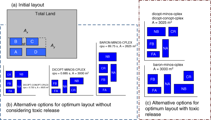
Figure 12.11 Optimum layouts for piping, land and toxic release risk minimization. Reprinted from Richart Vazquez‐Roman, Jin‐Han Lee, Seungho Jung, M. Sam Mannan, Optimum facility layout under toxic release in process facilities: A stochastic approach, Computers & Chemical Engineering, Vol 34, pp. 122–133. Copyright (2010), with permission from Elsevier.
Díaz‐Ovalle, Vázquez‐Román, and Mannan (2010) modified this problem based on the worst‐case toxic release scenario. They assumed that a set of facilities is already installed on the site and a new set of facilities need to be accommodated. The worst‐case scenario was defined as F type Pasquill‐Gifford wind stability, and wind speed of 6 m/s and 1.5 m/s.
Jung et al. (2011) further extended this study to systemically integrate fire and explosion scenarios in safety and economic analysis of plant layout optimization. The mathematical model is formulated by considering a grid‐based approach for single unit placement under the constraints of the risk score, cost, and separation distances. The impacts of blast overpressure from hazardous events such as boiling liquid expanding vapor explosion (BLEVE) and vapor cloud explosion (VCE) were simulated. Monte Carlo simulation is considered for the realistic representation of the weather conditions, which is used for determining the flammable gas dispersion zone. For a case of heptane and hexane distillation separation, the mathematical model becomes a mixed integer linear programming problem, which is solved using CPLEX. Jung also pointed out the limitations of the current advanced techniques and proposed a framework for solving such problem (2016). Figure 12.12 depicts the proposed framework. It recommends conducting QRA as a first step to determine the risk level, and then optimizing the program to select unit locations. In the final step, computational fluid dynamics modeling of hazardous releases were conducted for dispersion of materials and overpressurization due to the explosion. Similar studies have been conducted by Martinez‐Gomez et al. (2014), where they showed the effectiveness of solving a Multi‐Objective Mixed Integer Non‐Linear Programming (MO‐MINLP) problem in mitigating the risk via layout optimization.
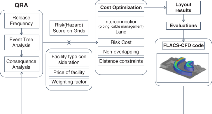
Figure 12.12 Flowchart for the proposed methodology. Kor J Chem Engg, Facility siting and plant layout optimization for chemical process safety, Vol 33, 2016: 1‐7, Seungho Jung, Copyright (2016) Korean Institute of Chemical Engineers, Seoul, Korea, With permission of Springer.
Domino effects often result in much more catastrophic subsequent damage, compared to the initial event. However, it is very difficult to determine the factors and relationships between initial events with another. So et al. (2011) introduced the concept of quantitative estimation of a domino effect in facility siting and formulated a framework for improved incident prevention based on proper design (López‐Molina et al., 2013) and also studied the principles to reduce the risk of a domino effect in plant layout.
Han et al. (2013) proposed a risk index approach to minimize risk to humans in optimizing process layout. A modified definition of individual risk is proposed. For a location “i,” person “k,” the modified risk is defined as
where, θ k is the fraction of time and P loc, i, k is the probability of the presence of that person in the ith location. Being a person in that place doesn't mean the person will die. Therefore, it is multiplied with the frequency of fatality, FoF i , which is defined as;
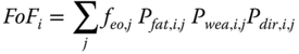
Here, f eo, j indicates incident frequency, P fat, i, j fatality rate, P wea, i, j weather condition, and P dir, i, j the directional effect. The authors optimized the siting of a dimethyl ether (DME) filling station, which consisted of four storage tanks, pump, compressor, dispersion and control room. Figure 12.13 presents the key findings of this study. Figure 12.13(a) indicates the individual risks against distance from equipment, whereas Figure 12.13(b) shows the risk map for a certain storage tank. Optimum locations for hazardous units are usually in places where the risk level is lowest.
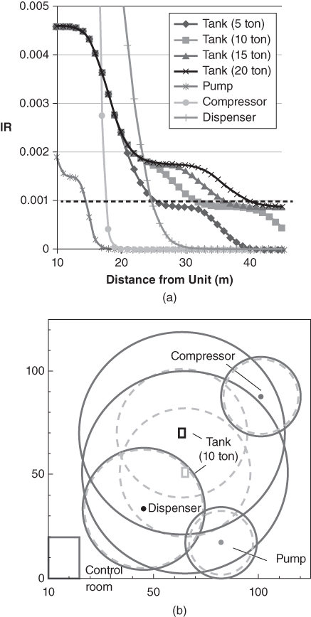
Figure 12.13 (a) Individual risks against distances from each equipment (b) Risk contours for storage tanks. Reprinted with permission from Industrial & Engineering Chemistry Research, Kyusang Han, Young Hun Kim, Namjin Jang, Hosoo Kim, Dongil Shin, En Sup Yoon, Risk index approach for optimal layout of chemical processes minimizing risk to humans, Vol 52 (22): 7274–7281. Copyright (2013) American Chemical Society.
Facility siting study is a complex mathematical problem, and as such oftentimes it is very difficult to communicate with upper management and convince them to pursue advanced techniques. James (2017) presented a best practice on how the resulting information of facility siting and layout optimization can be communicated. The most notable recommendations are using a visual aid to summarize issues and present solutions, historical facility siting fines, maintenance issues, and recommendations.
Lessons Learned from Past Incidents
During the Flixborough disaster (June 1, 1974), 18 of the 28 fatalities occurred in the control room. An estimated overpressure of 0.7 bar (10 psi), resulting from an explosion at 100 m distance, knocked out 1½ story roof of a 2½ storied control room. The building was constructed using a reinforced concrete frame, a brick panel with considerable size window. The control room was located in a building alongside a production block, amenities building, laboratory, and manager's office. Cable duct and electrical switchgear ran through above the control room. The occupant of the control room died because of the collapse of the roof. If a detailed facility siting and layout optimization study had been performed and appropriate recommendations implemented, the number of casualties could have been minimized during the Flixborough incident.
Another classic, but more recent incident, where injuries and the loss of human lives could have been minimized, by conducting a proper facility siting study, is the BP Texas City refinery incident on March 23, 2005. This incident caused 15 fatalities, 170 injuries, and major economic losses. The impact of the incident would have been much lower if proper spacing among units were allowed. The U.S. Chemical Safety and Hazard Investigation Board (CSB) has investigated the incident and recommended that facility siting should be addressed in the Process Hazard Analysis under the Process Safety Management program. The key learnings of this incident are facility siting issues regarding temporary buildings for reducing the risk of personnel during unit malfunctions and blast proofing of occupied buildings in hazard zones.
Relief System Design
Relief systems provide a means of controlled release of the flammable, toxic, or reactive materials in gas, liquid, or both phases, to a safe location during equipment failures, or operator errors, which leads to overpressurization of the tanks. It provides protection against damage of the overpressurizing equipment, minimizes the loss of materials, prevents damage to adjacent facility or units, reduces insurance premiums, and facilitates compliance with regulations. Recommended codes and standards such as API RP 520, 521, DIERS (Little, Sundmacher, and Kienle 1992; API 1997, 2000), are widely practiced.
The selection of relief devices is specific to its applications. The general classification falls into four broad categories: spring‐operated valves (conventional and balanced‐bellows), rupture disks, buckling‐pin valves, and pilot‐operated reliefs. Spring‐operated valves used in the liquid service are called relief valves, which begin to open at a set pressure and fully open at 25% overpressure. The safety valve is for gas service. The spring‐operated valve used for both liquid and gas service is called a safety relief valve. Rupture discs burst at the set pressure and remain open. Depending on the service, rupture discs need to be corrosion resistant; care is needed to avoid plugging, and discs are often installed in series with spring‐loaded relief valves. Buckling pin devices are similar to rupture discs but provide precise response to the set pressure. In a pilot‐operated relief, the main valve is controlled by a smaller pilot valve. When the pilot valve reaches the set pressure, it opens the main valve. This kind of relief device is preferred for the large relieving area.
Overpressurization of equipment or tanks can occur under various operating conditions, requiring various sizes of relief area. However, it is not practical to have multiple relief devices for multiple scenarios. Therefore, the worst‐case event is considered for relief sizing. Considerations of all relief scenarios need to be evaluated to ensure the adequacy of the relief system. Oversized relief devices cause problems known as “chatter” due to frequent opening and closing of the valves. This can significantly reduce the life of the valve. API RP 520 provides guidelines on the selection and installations of relieving devices. After an opening of a relief valve, the hazardous materials must be contained to prevent further unwanted events such as fire and explosion. As a result, the design of overflow header, the blow‐down tank, the subsequent condenser, scrubber, and flare stack should be able to handle the released mass.
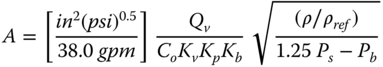
API RP 520 recommends the following formula for a conventional spring‐operated relief in liquid service.
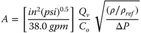
For a rupture disc in liquid service, the relief area is calculated by using
For conventional spring‐loaded reliefs in vapor or gas service, it is assumed the flow is choked flow, and therefore the relief area is calculated as follows.
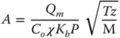
where,
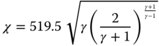
For a gas or vapor service, the above equation simplifies to
Toxic and Heavy Gas Dispersion
The most infamous example of toxic release is the Bhopal (1984) disaster, which killed more than 3,000 people and led to the ultimate sale and demise of Union Carbide. The 30‐ton leak of the hazardous intermediate chemical known as methyl isocyanate (MIC) caused the havoc. Fortunately, less hazardous materials are involved in natural gas processing. Nevertheless, there is a potential of toxic releases such as H2S and toxic refrigerants (e.g., NH3). In 1950, in Poza Rica, Mexico, due to the malfunctioning of a sulfur‐recovery unit that was processing 60 MMSCF natural gas per day, a 10 MMSCF per day gas stream was released to the environment which contained 16% H2S for 20 minutes (McCabe and Clayton 1952). The exposure caused 22 fatalities and sent 320 people to hospitals. These incidents emphasize the importance of consequence analysis, such as toxic and heavy gas dispersion studies, for further improvement in planning and designing facilities.
Dispersion models play a crucial role in the consequence analysis. It is an integral part in developing an emergency response plan for the surrounding community, modification in the design to eliminate hazards at the source, adding appropriate engineering barriers, reducing the inventories of hazardous materials, and detecting and monitoring for leaks to take actions. A wide variety of parameters affect the airborne transport of the released material in the downwind directions, e.g., wind speed, atmospheric stability, terrain types, the height of released location, and momentum and buoyancy of the release. High wind speed carries the substance downwind at a faster rate and enhances dilution. Atmospheric stability refers to the vertical mixing of the air due to the temperature gradient. In a stable condition, the sun cannot heat the ground as fast as it cools. Ground conditions affect the mixing and turbulence, and the wind profile with the height. The mixing is higher in areas with trees and buildings, whereas open areas such as lakes decrease it. Higher release height allows more dispersion and therefore reduces the ground level concentration. The buoyancy and momentum of the release also affect the effective release height and consequently affect the ground level concentration.
Air mixed gas becomes neutrally buoyant and disperses in a streamline. A plume model is used to describe the steady‐state concentration from a continuous release, whereas a puff model is used for the instantaneous release of material. A simplified mathematical model of neutrally buoyant dispersion of gas also known as the Gaussian model is given as follows (Crowl and Louvar 2011).
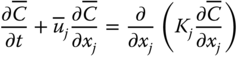
For a steady‐state release, the mass flux at any point is equal to the release rate (Qm). Thus, different scenarios such as steady‐state point release, puff release, non–steady state point release, wind and no‐wind conditions, and release location at a height and on the ground can be studied by solely modifying the above equations. The Pasquill‐Gifford model for weather conditions is the most popularly used model among the community. The accuracy and usefulness of this dispersion model greatly depends on the input (e.g., Qm) also known as source‐term (Ahammad, Liu, et al. 2016; Ahammad, Olewski, et al. 2016).
The Gaussian model is only valid for neutrally buoyant substances and limited to a dispersion distance of 0.1–10 km. The local concentration may exceed the estimated time average concentration. The effect of the structures on the ground is ignored even though it can significantly change the concentration estimates. Commercially available software (e.g., PHAST, CANARY) somewhat improves these limitations by incorporating semi‐integral models for source‐terms, ground structures and are validated against the large‐scale experimental releases (Pandya, Gabas, and Marsden 2012).
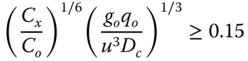
A dense gas (heavier than air) has higher damage potential than the neutrally buoyant one because its cloud slumps towards to ground and can blanket occupied areas. Britter and McQuaid (1988) developed a model by performing a dimensional analysis and experimental data for dense gas dispersion. The model works best for ground‐level releases and assumes no flashing or aerosol formation. The model is validated using the experimental data for flat terrain and rural area. As the gas moves in a downwind direction, the concentration of the released material decreases, resulting in a transition to a neutrally buoyant dispersion. To determine the transition location, the following criteria can be used (Crowl and Louvar 2011).
The limitations of integral and semi‐integral models are overcome by using CFD models. More accurate estimations are achievable using such tools. The effects of buildings or equipment in the dispersion path, simulation for the exact weather conditions of the site, incorporation of terrain properties such as hills and valleys are regularly considered in the modern dispersion calculations. CFD software such as FLACS is validated for dense gas (e.g., LNG) to conduct more accurate dispersion calculations (Hansen et al. 2010). (Cormier et al. 2009; Qi et al. 2010) have shown that ANSYS CFX can be used to faithfully simulate the LNG vapor cloud dispersion experimental study performed at the Mary Kay O'Connor Process Safety Center.
Fire and Explosion
The most frequent event of a serious nature in the process plant is fire, which occurs almost on a daily basis. It is usually thought to have less potential to cause damage compared to explosions or toxic release. However, under certain circumstances, a fire can lead to more catastrophic consequences, such as boiling liquid expanding vapor explosions (BLEVE) or secondary vapor cloud explosions. Failures of the critical structure or pipelines due to fire exposure could cause secondary releases and domino effects. In general, fire is categorized as jet fire, flash fire, pool fire, and fireball. In a natural gas processing plant, the expected type of fire would be NFPA class B (fire from flammable gas and combustible liquid) and class C (fire involving energized electrical equipment). Fire can be the cause and a consequence of explosion in such plant. Therefore, another convenient fire classification might be based on the type of fire, i.e., Type 1 (fires with no explosion), Type 2 (fires resulting from explosions), and Type 3 (fires resulting in explosions). Buildings, critical structures, and pipelines may need to be rated for intense radiative heat.
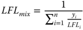
No fire can occur without the simultaneous existence of fuel gas, oxygen (i.e., air) and heat (i.e., ignition source). Flammability of a gas determines the concentration range within which a gas‐air mixture is combustible. Natural gas, which is predominantly methane, has a lower flammability limit (LFL) of 5% and upper flammability limit (UFL) of 15%. For mixtures of hydrocarbon stream, the flammability can be estimated using Le Chatelier equation (Chatelier 1891).
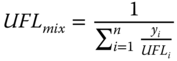
The temperature and pressure dependence of the flammability can be estimated using the following empirical correlations (Zabetakis, Lambiris, and Scott 1959; Zabetakis 1965).
The term “auto‐Ignition temperature” (AIT) refers to a minimum temperature above which flammable gas‐air mixture combustion occurs spontaneously. Releases from the process streams where the temperature is above AIT will catch fire spontaneously. Table 12.3 refers to the AIT of paraffinic compounds.
Table 12.3 Flammability limits and AIT of natural gas compounds (Mannan, 2012).
| LFL (Vol % in air) | UFL (Vol % in air) | AIT (°C) | LFL (Vol % in air) | UFL (Vol % in air) | AIT (°C) | ||
| Methane | 5.0 | 15.0 | 537 | n‐Heptane | 1.0 | 7.0 | 223 |
| Ethane | 3.0 | 12.5 | 515 | n‐Octane | 0.8 | 6.5 | 220 |
| Propane | 2.1 | 9.5 | 466 | n‐Nonane | 0.7 | 5.6 | 206 |
| n‐Butane | 1.8 | 8.5 | 405 | n‐Decane | 0.8 | 5.4 | 208 |
| n‐Pentane | 1.4 | 7.8 | 258 | H2S | 4.3 | 45.0 | 260 |
| n‐Hexane | 1.2 | 7.5 | 223 | NH3 | 16.0 | 25.0 | 651 |
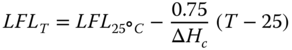
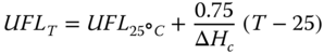
Figure 12.14 depicts the relationships between different flammability properties, e.g., LFL, UFL, AIT, flash point.
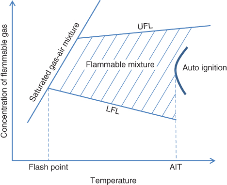
Figure 12.14 Flammability relationships.
There are numerous ignition sources in a natural gas processing plant, and it is practically impossible to eliminate all of them. Many of the fires can be attributed to well‐known ignition sources, such as electrical, smoking, friction, hot surface, hot works, mechanical sparks, and static charges.
U.S. regulations require that the radiant heat release from the fire should not be higher than 5kW/m2 at the plant boundary. Fire models are the essential component in studying the geometry and heat release rates. An excellent review of the LNG pool fire models can be found in the white paper published by the Mary Kay O'Connor Process Safety Center (MKOPSC 2008), which is based on a workshop held for industry experts. The basic fire models are empirical or semi‐empirical; for example, the following pool fire model (Thomas 1963) correlates the flame length to diameter ratio, L/D, with the mass burning rate m.
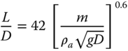
The actual fire scenario is quite different as many parameters interact with each other, e.g., wind speed, evaporation rate from the liquid pool, the shape of the pool, plume length, and tilt. Therefore, such models require experimental validations. Some notable large‐scale LNG pool fire experiments are China Lake experiments, Maplin Sand, Montoir, and Lake Charles.
The major identified research needs related to LNG pool fire modeling are large‐scale experiments (>35m), measurement data for large fires, and overcoming the limitations of the geometric structure model such as cylindrical fire (MKOPSC 2008). Well‐validated CFD models of pool fire are much more useful than the estimates of semi‐empirical models, and these models can overcome such limitations. Figure 12.15 depicts a case simulation using ANSYS CFX, where the temperature profile of the large storage tanks (e.g., T2) is studied for a domino effect.
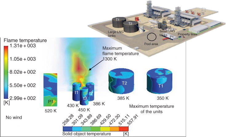
Figure 12.15 Maximum temperature distribution of flame and solid units for quiescent conditions. Reprinted from Muhammad Masum Jujuly, Aziz Rahman, Salim Ahmed, Faisal Khan, LNG pool fire simulation for domino effect analysis, Reliability Engineering & System Safety, Vol 143, pp. 19‐29. Copyright (2015), with permission from Elsevier.
Generally, leaks from a pressurized vessel would result in a jet fire, but they can also occur from a wide variety of situations. A low‐velocity jet flame is usually attached to the release point, but high‐velocity flame can be detached. If the velocity increases, it may become unstable and lift off, or get extinguished. The impingement distance of a jet flame can be more than 50 m. API correlates the impingement length L (m) with the mass flowrate ![]() (kg/s) as follows.
(kg/s) as follows.
Computer code SAFETI models jet fire based on API RP 521 (Cook, Bahrami, and Whitehouse 1990). The relationships are given below.
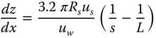
The effects of wind on flame bending are also considered in the geometry of the flame. For a wind velocity of u w , jet velocity of u s , the rate of vertical height z in respect to the horizontal distance x can be expressed as:
Bagster and Schubach (1996) proposed the following correlations for methane jet fire dimensions.
External heating of a tank could lead to a BLEVE and fireball. TNO suggests the following model estimate the dimension and heat flux received in a certain distance from a fireball (TNO 1997).
An explosion results from the rapid release of energy at a very high rate to cause local energy accumulation, which is dissipated via pressure wave, projectiles, thermal radiation, and acoustic energy. A shock wave or pressure wave faster than the reaction front propagates through the air. In a deflagration explosion, the reaction front moves at a speed less than sonic, and the shock wave moves at sonic velocity. In the case of a detonation, both the reaction front and the shock wave move at a speed higher than sonic.
The damage associated with the explosion depends on the maximum blast overpressure and its duration. Generally, an overpressure of 0.3 psig is considered to be a “safe distance.” Overpressures of 1.0 psig can cause partial demolition to a house. At 3 psig, heavy machines in the industrial building suffer minor damage, and steel frame buildings distort and can be pulled away from the foundation. At 10 psig, total destruction of buildings and heavy machine damage is probable.
The most commonly used explosion models are TNT and TNO multi‐energy. In the TNT model, the energy released from the explosion is converted to equivalent TNT mass, and then empirical scale law is used to determine the blast overpressure at certain distances. The energy released in a VCE is due to the burning of dispersed gas over a large volume; therefore, the TNT model overpredicts the result for VCE in the near distance and underpredicts at large distances. Confinement and congestion in the facility increase the severity of the explosion. In the TNO method, the degree of confinement/congestion and semiempirical correlations are used to determine blast overpressure.
Tang and Baker (1999) performed a series of CFD simulations to study VCE for detailed real scenarios without simplifications. Material reactivity, flame expansion, and obstacle density are used to characterize flame speed. The blast pressure decay curves were generated from the CFD simulations. The validations are carried out for vapor cloud detonation, supersonic deflagration, and subsonic deflagration. A more detailed description is given by Tang and Baker (1999).
Effective Mitigation System
An effective mitigation system can significantly reduce the consequences of the loss of primary containment event. Such systems should be based on the principle of detection–decision–action. The system detects the loss of primary containment, gas release, and presence of fire to determine appropriate measures that need to be taken. The system then actuates the mitigation action, such as a water curtain to disperse flammable gas or absorb toxic gas or foam to reduce the excessive pool vaporization thus reducing the heat flux. The mitigation system can be automatic, but human action often plays a crucial role in the detection and decision‐making steps. Therefore, the reliability of mitigation system becomes dependent on the reliability of human actions.
The effectiveness of the detection process depends on the placement of sensors near the leak locations. Unfortunately, detector placement has traditionally been done by following rules of thumb rather than analyzing the propagation of the event, e.g., the dispersion behavior of gas. Benavides‐Serrano, Mannan, and Laird (2015) presented a novel approach regarding the placement of gas detectors and compared its efficacy with random approach (RA), volumetric approach (VA), the minimization of the distance between the detectors and the leak sources approach (MSDP), the greedy scenario coverage approach (GC), maximum covering location problem (MCLP) approach, and a novel stochastic programming formulation considering unavailability and voting effects (SP‐UV). In the random approach (RA), N number of detectors is randomly placed in L number of possible locations. In the volumetric approach (VA), the goal is to detect a vapor cloud, which is assumed to grow spherically before getting larger than a predetermined diameter. Therefore, the number of detectors N is calculated from the facility volume, and the placement is carried out by either following a regular or a staggered pattern. In the minimum source distance problem (MSDP), the detectors are placed near the potential leak location, a method which conjectures that the effectiveness of the mitigation system will depend on the earlier detection. Placement locations are determined based on the rule of thumb industry practice. A greedy coverage algorithm (GC) and maximum coverage location problem (MCLP) are based on the principle of maximum release scenario coverage. In the GC approach, a simple rule is followed where at each stage of placement the candidate detector location should cover the largest number of uncovered leak scenarios. Once all scenarios are covered, redundant sensors are placed until each scenario is covered k times. In the MCLP approach, a weighted sum of the covered scenarios is maximized by selecting most of the candidate locations and therefore avoiding suboptimal greedy placement approach (Church and Revelle 1974). A stochastic programming formulation originally developed by Legg et al. (2012) is modified for SP‐UV approach. The assumptions of detector failures such as false negative or false positive alarms, and detector redundancy for emergency work are incorporated in the formulation of SP‐UV approach by Benavides‐Serrano, Mannan and, Laird (2015). Figure 12.16 depicts the effectiveness of the gas detection for different placement approaches. For a subset of randomly selected scenario, the SP‐UV formulations give the quickest response with the fewest number of sensors.
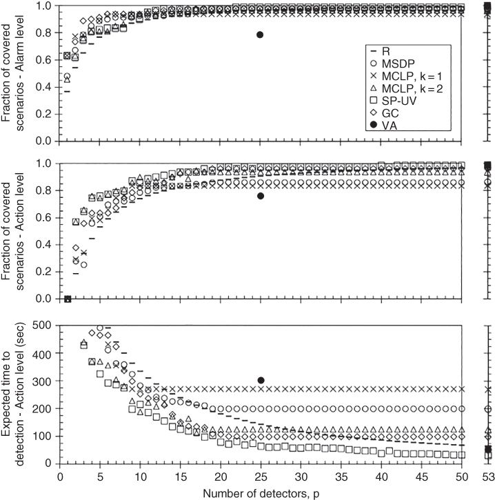
Figure 12.16 Effectiveness of gas detector placement methods under a randomly selected subset of scenarios. Reprinted from Vol 35, A.J. Benavides‐Serrano, M.S. Mannan, C.D. Laird, A quantitative assessment on the placement practices of gas detectors in the process industries, Journal of Loss Prevention in the Process Industries, pp. 339–351. Copyright (2015), with permission from Elsevier.
The water curtain has been recognized as one of the most effective and economical systems for dispersing dense gas, absorbing toxic components, and preventing flammable gas from reaching ignition sources. It has been proven to enhance the dispersion and reduce the safety distance for LNG vapors. Rana and Mannan (2010) performed an experimental study of the physical mechanisms of water curtains dispersing LNG vapor cloud. A flat fan and full conical upward water sprays were used for these tests. The results indicate that the water curtain reduced LNG vapor concentration and pushed the vapor in the upward direction as shown in Figure 12.17.
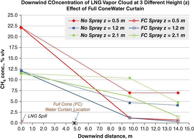
Figure 12.17 Downwind concentration at three different heights with and without full‐cone water curtain. Reprinted from Morshed A. Rana, M. Sam Mannan, Forced dispersion of LNG vapor with water curtain, Journal of Loss Prevention in the Process Industries, Vol 23, pp. 768‐772. Copyright (2010), with permission from Elsevier.
Kim et al. (2013) applied CFD using the Eulerian‐Lagrangian spray model to evaluate global key parameters, e.g., droplet characteristics, installation distances, nozzle configurations, and air entrainment rates for designing effective forced mitigation system. Figure 12.18 shows how the LNG vapor concentration decreases with the water spray installation distance.
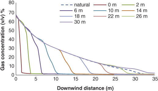
Figure 12.18 LNG vapor concentration in downwind distances at ground level for different water spray installation distances. Reprinted from Vol 26, Byung Kyu Kim, Dedy Ng, Ray A. Mentzer, M. Sam Mannan, Key parametric analysis on designing an effective forced mitigation system for LNG spill emergency, Journal of Loss Prevention in the Process Industries, pp. 1670‐1678. Copyright (2013), with permission from Elsevier.
Yun, Ng, and Mannan (2011) studied high expansion foam as a mitigating measure for a boiling and evaporating LNG pool and subsequent fires. They studied the temperature changes in the pool and the fire and the profile of the radiant heat fluxes for determining the effectiveness of foam application. The experiments were carried out at the Brayton Fire Training Field, College Station Texas. LNG is poured into a 78.5 m3 concrete pool, which was instrumented with 166 thermocouples, and radiometers. A portable weather station was used to record experimental conditions. Figure 12.19 shows one of the results of this experimental series. After foam application, the flame height was significantly reduced from 17 m to 6 m and the radiative heat flux at 15 m downwind distance was reduced from 14k W/m2 to 1 kW/m2.
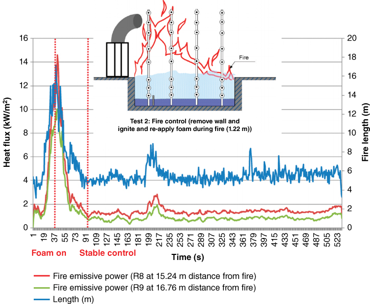
Figure 12.19 Fire length and heat flux for the experimental study of fire radiation mitigation by using high expansion foam. Reprinted with permission from Industrial & Engineering Chemistry Research, Vol 50 (4), Yun, G., Ng, D. and Mannan, M.S., Key findings of liquefied natural gas pool fire outdoor tests with expansion foam application: 2359‐2372, Copyright (2011) American Chemical Society.
Regulatory Program and Management Systems for Process Safety and Risks
Historically, the approach towards process safety has been reactive rather than proactive. Well‐publicized catastrophic events have shaped the process safety regulations and technology developments (Mannan et al. 2016). Figure 12.20 pictorially shows the evolution of process safety technology, management systems, standards, and regulations in the context of well‐publicized process safety incidents.
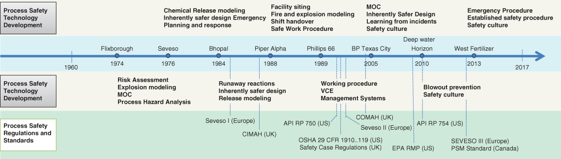
Figure 12.20 Major incidents and evolution of process safety technology, management system and regulations.
The European Union adopted the Seveso Directives on June 24, 1982, after a serious incident in Seveso, Italy. The amendments to the Seveso Directives resulted as a regulatory response to incidents at Basel, Switzerland (1986), and Toulouse, France (2001), to formulate Seveso II (1996) and Seveso III (2012).
Following the 1974, Flixborough incident, the UK government responded by promulgating and implementing Control of Industrial Major Accident Hazards (CIMAH) regulations. The key objective of CIMAH and SEVESO I was to address the direct environmental impact of major incidents. The Control of Major Accident Hazards (COMAH) regulation came into effect from 1999 and was later amended in 2005. This regulation is also known as the Safety Case. Australia also adopted regulations similar to the Safety Case of the UK.
In the United States, process safety regulations became a statutory requirement in 1990 under the Clean Air Act Amendments, which directed the Occupational Safety and Health Administration (OSHA) and the U.S. Environmental Protection Agency (EPA) to establish regulations, to protect workplace employees, the public, and environment, respectively. As a result, in 1992, OSHA promulgated the Process Safety Management (PSM) regulations for facilities handling flammable and toxic chemicals over specified limits. It also recommended adherence to recognized and generally accepted good engineering practice (RAGAGEP). Industry associations such as the American Petroleum Institute (API) published standards such as API 750 and API 754 as proactive measures to improve safety. While OSHA regulations were focused on plant personnel and equipment safety, the EPA fulfilled its mandate by promulgating the Risk Management Program (RMP) in 1996 to address public safety and environmental damage due to loss‐of‐containment incidents. Both the PSM and RMP regulations are very similar regarding the Prevention Program and Emergency Planning requirements. The RMP regulation additionally requires an offsite consequence analysis, which includes worst‐case and alternative‐scenario analysis and incident history. In addition, the EPA RMP regulation requires the development of a risk management plan (RMPlan), which must be submitted to the EPA. Table 12.4 compares the various elements of the PSM and RMP regulations. Other U.S. federal regulations that are relevant to Chemical Process Safety are described by Crowl and Louvar (2011). In Canada, the Process Safety Management Division (PSMD) of the Canadian Society for Chemical Engineering (CSChE) published PSM standards in 2012 in accordance with the USA PSM regulations.
Table 12.4 Elements of US PSM and RMP regulations.
| OSHA PSM Elements | EPA RMP Elements |
| Employee participation Process safety information Process hazard analysis Operating procedure Training Contractors Pre‐startup safety review (PSSR) Mechanical integrity Hot Work Permit Management of change (MOC) Incident investigation Emergency response and planning Compliance audits Trade secrets – |
– Process safety information Hazard evaluation Standard operating procedure Training – Pre‐Startup Safety Review (PSSR) Maintenance – Management of change (MOC) Accident investigation Emergency response Safety audits – Offsite consequence analysis
|
In the United States, natural gas and LNG facilities are regulated by the federal government under regulations promulgated by the Pipeline and Hazardous Materials Administration (PHMSA) of the U.S. Department of Transportation (DOT). Current DOT regulations (49 CFR, part 193) on LNG are outlined in NFPA 59A, “Standard for production, storage, and handling of liquefied natural gas.” The original version (2001 edition) of this regulation is prescriptive and inflexible. The later edition (2009) offers risk‐based evaluation requirements for land‐based facilities. Raj and Lemoff (2009) studied the regulation and proposed alternative methods for performing better LNG facility siting risk assessment. They also compared the practices in other countries, particularly in Europe, and provided recommendations.
Concluding Remarks
Being a relatively new area of science and engineering, the scope of future research and development in process safety is very wide. However, there are several outstanding challenges that need to be addressed to advance process safety performance (Mannan et al. 2016). Some of the key issues are as follows:
- • Historical failure data are not good enough to portray the current picture of risk in the plant. Real‐time management data, or operational data, or data‐independent mechanistic approaches based on first principles are needed throughout the industry.
- • Despite proper facility siting and plant layout optimization, a severe consequence of rare events can occur, due to the migration of population centers towards the plant. Thus, land‐use planning based on engineering calculations should be incorporated in the permitting of industry, housing, business centers, education centers, and hospitals.
- • Establishment of a chemical incident surveillance system for process safety incidents is an essential necessity for appropriate tracking of incidents for trending analysis, identification of improvement needs, and other actions. There are very limited data sources to distinguish the efforts and returns in mitigating risks. The surveillance system can also be used to create a knowledge base for improving infrastructure, planning, enhancing the response capability, and incorporating lessons learned into the system.
- • Regulations are the minimum requirement, whereas individual companies should strive for the best‐in‐class safety culture (Mannan, Mentzer, and Zhang 2013; Mannan et al. 2016). However, the regulations should be based on risk‐based studies and sound science. Once adopted, regulations must be enforced strictly to ensure compliance. A cost‐effective certified third‐party enforcement program can be adapted to reduce the burden of the regulators.
- • Building process safety competency for the leadership, plant management, engineers, operators, and contractors is the key to success in preventing and mitigating process safety incidents. Academic research and dissemination of knowledge to students and practitioners alike will also go a long way in paving the pathway for preventing future incidents (Olewski et al. 2016). Risk communications to the surrounding community to generate awareness and preparation for response to potential events is another essential need for twenty‐first‐century society.
Nomenclature
Symbols
- A x , A y
- length of subunits in the x, y‐direction, m
-

- mean concentration of the substance, kg/m3
- C l
- land cost per square meter, $/m2
- C o
- concentration at the source, kg/m3
- C o
- discharge coefficient, dimensionless
- C p
- cost of pipe, $/m
- C pp
- compensation cost per fatality, $
- C x
- concentration at x distance downwind, kg/m3
- D c
- characteristics dimension of the release, m
- F view
- geometric view factor, radian
- K b
- backpressure correction factor, dimensionless
- K j
- eddy diffusion co‐efficient, dimensionless
- K p
- overpressure correction factor, dimensionless
- K v
- viscosity correction factor, dimensionless
- P b
- backpressure, psia
- P dir, i, j
- factor for directional effect
- P fat, i, j
- factor for fatality rate
- P s
- expected population in the facility
- P s
- set pressure, psia
- P wea, i, j
- factor for weather condition
- Q m
- mass flowrate, discharge rate, kg/s
- Q v
- volumetric flowrate, m 3/s
- R S
- radius of flame, m
- d i, j
- center‐to‐center distance between two units, m
- f eo, j
- incident frequency, Hz
- f i, r
- frequency of the type of release, r, in unit i
-

- mass flowrate, kg/s
- t l
- expected lifespan of the plant, yr
- u s
- jet velocity, m/s
- u w
- wind velocity, m/s
- x j
- distance in jth co‐ordinate, m
- y i
- flammable composition, volume % in air
- ρ a
- density of air, kg /m3
- τ a
- atmospheric transmissivity, dimensionless
- Fr
- Froude number, dimensionless
- h
- hazard rate, Hz
- M
- molecular weight, gm
- s
- distance along the centerline of fire, m
- u i
- velocity in ith direction, m/s
- ΔH c
- heat of combustion, J/kg
- A
- pressure relief area, in 2
- D
- diameter of pool fire, m
- H, D
- height and diameter of jet fire, m
- L
- pool fire flame height, m
- P
- pressure, Pa
- P
- probability of failure of equipment or component, dimensionless
- R
- reliability of an equipment, dimensionless
- S, A, A ′
- a system, its good state and failed state
- SEP
- surface emissive factor, kW/m2
- T
- temperature, K
- d
- hole diameter, m
- f
- failure density function, Hz
- m
- flammable mass of fireball, kg
- m
- Mean Time To Failure (MTTF), or Mean Time Between Failure (MTBF), s
- n
- total numbers of equipment
- r
- total numbers of functional equipment
- r, h
- radius and liftoff height of fireball, m
- t
- duration of fireball, m
- t
- time period, s
- u
- wind speed, m/s
- x
- horizontal distance, m
- z
- compressibility factor, dimensionless
- z
- vertical height, m
- γ
- heat capacity ratio
- λ
- a constant failure rate, Hz
- ρ/ρ ref
- specific gravity, dimensionless
Subscripts
- f
- identify as failed
- i, j
- index variable
- l
- lifetime
- mix
- mixture
- T, P
- value at Temperature T or Pressure P
Constants
- g
- 9.8 m/s2
References
- Ahammad M, Liu Y, Olewski T, Vechot L, MS. 2016. Application of computational fluid dynamics (CFD) in simulating film boiling of cryogens. Indus Engg Chem Res, 55: 7548–7557. doi: 10.1021/acs.iecr.6b01013.
- Ahammad M, Olewski T, Véchot LN, Mannan MS. 2016. A CFD based model to predict film boiling heat transfer of cryogenic liquids. J Loss Preven Proc Indus, 44: 247–254. doi: 10.1016/j.jlp.2016.09.017.
- API. 1997. RP‐521, Guide for pressure‐relieving and depressuring systems. American Petroleum Institute, Washington DC.
- API. 2000. RP‐520, Sizing, Selection and Installation of Pressure‐Relieving System in Refineries. American Petroleum Institute.
- API. 2010. Process safety performance indicators for the refining and petrochemical industries. Washington DC.
- Bagster DF, Schubach SA. 1996. The prediction of jet‐fire dimensions, J Loss Preven Proc Indus, 9(3): 241–245.
- Benavides‐Serrano AJ, Mannan MS, Laird CD. 2015. A quantitative assessment on the placement practices of gas detectors in the process industries. J Loss Preven Proc Indus, 35: 339–351.
- Britter R, McQuaid J. 1988. Workbook on the dispersion of dense gases. Health and Safety Executive. Available from: http://publications.eng.cam.ac.uk/332178/.
- CCPS. 2003. Guidelines for facility siting and layout. New York: Center for Chemical Process Safety of the AIChE (CCPS/AIChE).
- Le Chatelier H. 1891. Estimation of firedamp by flammability limits. Annals o Mines, 19 (8), 388–395.
- Church R, Revelle C. 1974. The maximal covering location problem. Papers of the regional Science Association, 32. Available from: http://www.geog.ucsb.edu/∼forest/G294download/MAX_COVER_RLC_CSR.pdf.
- Cook J, Bahrami Z, Whitehouse RJ. 1990. A comprehensive program for calculation of flame radiation levels. J Loss Preven Proc Indus, 3(1): 150–155.
- Cormier BR, Qi R, Yun G, Zhang Y, Mannan MS. 2009. Application of computational fluid dynamics for LNG vapor dispersion modeling: a study of key parameters. J Loss Preven Proc Indus, 22(3): 332–352.
- Crowl D, Louvar JF. 2011. Chemical process safety: fundamentals with applications. 3rd ed. Boston: Pearson Education.
- Díaz‐Ovalle C, Vázquez‐Román R, Mannan MS. 2010. An approach to solve the facility layout problem based on the worst‐case scenario. J Loss Preven Proc Indus, 23(3): 385–392.
- Dweck J, Boutillon S, Asbill S, Brennan LLP. 2004. Deadly LNG incident holds key lessons for developers, regulators. Pipe Gas J, (May).
- Dyadem Press. 2003.Guidelines for failure mode and effects analysis for automotive, aerospace and general manufacturing industries. Dyadem Press. Available from: https://www.crcpress.com/Guidelines‐for‐Failure‐Mode‐and‐Effects‐Analysis‐FMEA‐for‐Automotive/Press/p/book/9780849319082.
- Han K, Kim YH, Jang N, Kim H, Shin D, Yoon ES. 2013. Risk index approach for the optimal layout of chemical processes minimizing risk to humans. Indus Engg Chem Res, 52(22): 7274–7281.
- Hansen OR, Gavelli F, Ichard M, Davis SG. 2010. Validation of FLACS against experimental data sets from the model evaluation database for LNG vapor dispersion. J Loss Prevent Proc: 857–877.
- Hirschberg S, Burgherr P, Spiekerman G, Dones R. 2004. Severe accidents in the energy sector: comparative perspective. J Haz Mat, 111(1–3): 57–65.
- James M. 2017. The eye opener: Preparing for and performing facility siting to best communicate with upper management. Proc Safety Prog, 36 (2): 158–164.
- Jung S. 2016. Facility siting and plant layout optimization for chemical process safety. Kor J Chem Engg, 33(1): 1–7.
- Jung S, Ng D, Diaz‐Ovalle C, Vazquez‐Roman R, Mannan M S. 2011. New approach to optimizing the facility siting and layout for fire and explosion scenarios. Indus Engg Chem Res, 50(7): 3928–3937.
- Khan F, Abunada H, John D, Benmosbah T. 2009. Development of risk‐based process safety indicators. Proc Safe Prog, 29(2): 133–143.
- Khan F, Hashemi SJ. 2017. Chapter One ‐ Introduction. In: Methods in chemical process safety. Elsevier. p 1–36.
- Kim BK, Ng D, Mentzer RA, Mannan MS. 2013. Key parametric analysis on designing an effective forced mitigation system for LNG spill emergency. J Loss Preven Proc Indus, 26(6): 1670–1678.
- Legg SW, Benavides‐Serrano AJ, Siirola JD, Watson JP, Davis SG, Bratteteig A, Laird CD. 2012. A stochastic programming approach for gas detector placement using CFD‐based dispersion simulations. Comput Chem Engg, 47: 194–201.
- Lewis D. 1980. The Mond fire, explosion and toxicity index applied to plant layout and spacing. Loss Prevent, 13: 20–26.
- Liaw H‐J. 2016. Lessons in process safety management learned in the Kaohsiung gas explosion accident in Taiwan. Proc Safe Prog, 35(3): 228–232.
- Little A, Sundmacher K, Kienle A. 1992. Emergency relief system design using diers technology: the design institute for emergency relief systems (DIERS) Project Manual.
- López‐Molina A, Vázquez‐Román R, Mannan MS, Félix‐Flores MG. 2013. An approach for domino effect reduction based on optimal layouts. J Loss Preven Proc Indus, 26(5): 887–894.
- Mannan MS, Mentzer RA, Zhang J. 2013. Framework for creating a best‐in‐class safety culture. J Loss Preven Proc Indus, 26(6): 1423–1432.
- Mannan MS, Reyes‐Valdez O, Jain P, Tamim N, Ahammad M. 2016. The evolution of process safety: current status and future directions. Ann Rev Chem Biomolec Engg, 7(1), 000−000.
- Mannan MS, West HH, Berwanger PC. 2007. Lessons learned from recent incidents: Facility siting, atmospheric venting, and operator information systems. J Loss Preven Proc Indus, 20(4–6): 644–650.
- Mannan MS. 2012. Lees' loss prevention in the process industries. 4th edn. Edited by S. Mannan. Butterworth‐Heinemann.
- Martinez‐Gomez J, Nápoles‐Rivera F, Ponce‐Ortega JM, Serna‐González M, El‐Halwagi MM. 2014. Siting optimization of facility and unit relocation with the simultaneous consideration of economic and safety issues. Indus Engg Chem Res, 53 (10): 3950–3958.
- Masum Jujuly M, Rahman A, Ahmed S, Khan F. 2015. LNG pool fire simulation for domino effect analysis. Reliab Engg Sys Safe, 143: 19–29.
- McCabe LC, Clayton GD. 1952. Air pollution by hydrogen sulfide in Poza Rica, Mexico: an evaluation of the incident of Nov. 24, 1950. Arch Indus Hyg Occup Med, 6(3): 199–213.
- MKOPSC. 2008. LNG pool fire modeling. College Station. Available from: http://psc.tamu.edu/files/links/lng‐white‐paper‐on‐pool‐fire‐modeling/LNG_White_Paper.pdf
- Olewski T, Ahammad M, Quraishy S, Gan N, Vechot LN. 2016. Building process safety culture at Texas A&M University at Qatar: a case study on experimental research. J Loss Preven Proc Indus, 44: 642–652.
- Pandya N, Gabas N, Marsden E. 2012. Sensitivity analysis of Phast's atmospheric dispersion model for three toxic materials (nitric oxide, ammonia, chlorine). J Loss Preven Proc Indus, 25(1): 20–32.
- Peekema RM. 2013. Causes of natural gas pipeline explosive ruptures. J Pipe Sys Engg Prac, 4(1): 74–80.
- Qi R, Ng D, Cormier BR, Mannan MS. 2010. Numerical simulations of LNG vapor dispersion in Brayton Fire Training Field tests with ANSYS CFX. J Haz Mat, 183(1–3): 51–61.
- Raj PK, Lemoff T. 2009. Risk analysis based LNG facility siting standard in NFPA 59A. J Loss Preven Proc Indus, 22(6): 820–829.
- Rana MA, Mannan MS. 2010. Forced dispersion of LNG vapor with water curtain. J Loss Preven Proc Indus, 23(6): 768–772.
- Richards F. 2013. Failure analysis of a natural gas pipeline rupture. J Fail Anal Prevent, 13(6): 653–657.
- So W, Kim Y‐H, Lee CJ, Shin D, Yoon ES. 2011. Optimal layout of additional facilities for minimization of domino effects based on worst‐case scenarios. Kor J Chem Engg, 28(3): 656–666.
- Tang MJ, Baker QA. 1999. A new set of blast curves from vapor cloud explosion. Proc Safe Prog, 18(4): 235.
- Thomas PH. 1963. The size of flames from natural fires. Symposium (International) on Combustion, 9(1): 844–859.
- TNO. 1997. Methods for the calculation of physical effects. 3rd ed. Edited by V. den Bosch and R. A. P. Weterings. Hague: Gevaarlijke Stoffen. Available from: http://content.publicatiereeksgevaarlijkestoffen.nl/documents/PGS2/PGS2‐1997‐v0.1‐physical‐effects.pdf.
- Vázquez‐Román R, Lee J‐H, Jung S, Mannan MS. 2010. Optimal facility layout under toxic release in process facilities: a stochastic approach. Comput Chem Engg, 34(1): 122–133.
- Wang M. 2012. Normalization of process safety metrics. Texas A&M University. MS Thesis.
- Yun G, Ng D, Mannan, MS. 2011. Key findings of liquefied natural gas pool fire outdoor tests with expansion foam application, Indus Engg Chem Res, 50(4): 2359–2372.
- Zabetakis MG. 1965. Fire and explosion hazards at temperature and pressure extremes. In: AICHE ‐ ICHEME symposium Series ‐2: 99–104.
- Zabetakis MG, Lambiris S, Scott GS. 1959. Flame temperatures of limit mixtures. in 7th Symposium on Combustion. London: Butterworths.