20
Natural‐Gas‐Based SOFC in Distributed Electricity Generation: Modeling and Control
Gerald S. Ogumerem1,2, Nikolaos A. Diangelakis1,2, and Efstratios N. Pistikopoulos1,2
1Artie McFerrin Department of Chemical Engineering, Texas A&M University, USA
2Texas A&M Energy Institute, Texas A&M University, USA
Chapter Menu
- 20.1 Introduction
- 20.2 Mathematical Model
- 20.3 Simulation
- 20.4 Multiparametric Model Predictive Control (mpMPC)
- 20.5 Closed‐Loop Validation and Results
- 20.6 Conclusion
20.1 Introduction
The recent global natural gas production increase and its low price in the United States has led to an increase in the utilization of natural‐gas‐based power generation (U.S. Energy Information Administration and U.S. Department of Energy 2011). Some studies have estimated the Ultimately Recoverable Resources (URR) of natural gas to be between 10,700 and 18,300 EJ, for conventional sources and 4,250 to 11,000 EJ for unconventional sources while the peak yearly natural gas recovery period is estimated between 2025 and 2066 at 140 to 217 EJ/y (Al‐Fattah and Startzman n.d.; U.S. Energy Information Administration and U.S. Department of Energy 2011; Mohr and Evans 2011). Natural gas is a feedstock for several industrial processes. Some of them convert natural gas to more valuable chemicals. Catalytic steam reforming is a popular industrial process for converting natural gas to syngas, and other valuable chemicals for other industrial processes. The main routes for converting natural gas to power includes converting its chemical energy (directly or indirectly) to thermal, kinetic or electrical energy. Internal combustion engines (ICE) and gas turbines are the most popular equipment for converting natural gas to kinetic and/or thermal energy, through combustion. The kinetic energy is subsequently converted to electrical energy, and the thermal energy is typically harnessed through an integrated system to improve the overall efficiency of the system through steam cycles. The use of natural gas for (distributed) electricity generation is gaining traction, currently propelled by low natural gas prices (U.S. Energy Information Administration and U.S. Department of Energy 2011). Figure 20.1 shows a projected increase in the use of natural gas (NG) for various activities including electricity generation (U.S. Energy Information Administration and U.S. Department of Energy 2011).
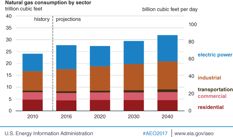
Figure 20.1 Natural Gas Consumption by Sector.
Over the years, there have been reports of increasing greenhouse gas (GHG) emissions, which have been correlated with the increasing fossil fuel usage. This has driven recent interest in alternative, environmentally benign energy sources. Comparatively natural gas has less adverse impact to the environment than other fossil fuels, and it is generally accepted as a good transition energy source (Burnham et al. 2011). The composition of natural gas varies significantly based on recovery locations, but methane is its major component, usually more than 80% of the total volume. Methane, is one of the GHGs, the combustion natural gas yields CO2 which is also a GHG. Emissions from leaks in natural gas production equipment contributes about 40% of estimated national emission of methane (US NETL 2013). Combustion of NG to produce energy generates about 117 pounds of CO2 per unit of heat (Million Btu equivalent) produced.
Coal produces more than 200 pounds of CO2 per million Btu while distillate fuel oil produces more than 160 pounds per million Btu equivalent (US EIA 2016). This and its lower impurity content makes NG a cleaner fossil energy source. The energy content of fuels can be categorized by their energy density. The energy density metric can be either gravimetric (energy content per weight) or volumetric (energy content per volume) (Hore‐Lacy 2006). Table 20.1 below shows a list some fuel types and their gravimetric energy density.
Table 20.1 Energy Density of Various Energy Sources.
|
Fuel Type |
Energy Density (MJ/kg) |
Typical uses |
| Biodiesel | 38 | automotive engine |
| Coal | 24 | Power plants, Electricity generation |
| Diesel | 45 | Diesel engines |
| Gasoline | 46 | Gasoline engines |
| Natural gas | 55 | Household heating, Electricity generation |
| Uranium‐235 | 3, 900, 000 | Nuclear reactor electricity generation |
| Wood | 16 | Space heating, Cooking |
Source: (Hore‐Lacy 2006).
20.1.1 Distributed Energy Production
Technology developments and environmental concerns are changing electricity generation and transmission. Smaller more distributed generating stations are replacing larger centralized generating facilities (Lasseter 2007). Technologies like fuel cells (FC), internal combustion engines (ICE), wind turbines (WT), gas turbines (GT), and photovoltaics (PV) and a combination of any of these, make up the variety used in most distributed system. These technologies also create avenues for process intensification that would be rather more expensive or unnecessary if applied to centralized generating systems. Distributed electricity‐generating systems have numerous advantages over centralized electricity‐generating systems. Their ability to be modularized increases their efficiency and flexibility. Cogeneration units like ICE‐based combined heat and power (CHP) can produce heat and electricity in a single process without major changes in fuel utilization, thereby increasing the efficiency of the system. Centralized power production units would usually have a minimum required load to be in operation, and the power generated is more than the required amount to compensate for the losses in transmission (Diangelakis and Pistikopoulos 2017). However, in distributed power production units, which are usually modularized units, there is less minimum‐required power production, which thus avoids large excess power production and therefore is cost effective and environmentally friendly. Distributed electricity production systems provide the opportunity to adopt renewable energy resources. The use of distributed solar and wind energy systems has gained a lot of interest. NG can have a significant contribution to the development of distributed systems. Technologies like the internal reforming solid oxide fuel cell (IR SOFC) use NG to produce electricity. Most residential units have existing NG supply lines for heating and other domestic activity, which makes the transition from a centralized electricity grid power production to a distributed IR SOFC electricity provision seamless.
20.1.2 Solid Oxide Fuel Cell (SOFC) Overview
Fuel cell technologies have received much attention in the last decade, with the polymer electrolyte membrane (PEMFC) fuel cell receiving the most due to its relevance in the transportation sector. Consequently, SOFC technology is not new; however, its use for distributed power generation in small to medium scale is still under testing and is yet to reach 40,000 hours of operation (the estimated life time of a SOFC unit) (Riensche et al. 1998).
Stand‐alone SOFC systems have efficiencies ranging from 40% to 55%. Combining the SOFC with a cogeneration of high‐grade thermal energy in a combined heat and power (CHP) system could increase its overall efficiency to approximately 80% (Hawkes and Leach 2005). With its attractive features, one would expect the SOFC to be an important technology for distributed power generation or an auxiliary power unit (APU). However, the commercialization of SOFC has been plagued by its financial implications. Studies by Jin et al. (2004) show that it takes about $8,738 to produce a 5 kW SOFC unit that uses diesel as fuel (Battelle 2014). This estimate is for the Balance of Plant (BOF) of an SOFC with an external reformer (see section 20.1.4) and a modular desulfurizing unit. As shown in Figure 20.2, the major cost‐contributing factors are the heat transfer unit and the electronic and controls units.
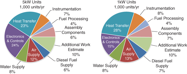
Figure 20.2 Cost Distribution for a 1kW SOFC plant and a 5kW SOFC plant.
Like other fuel cells (FC), SOFC uses hydrogen and oxygen to produce electricity. On the contrary to other FC alternative, the SOFC can use NG as fuel, a characteristic that makes this technology very attractive in areas with pre‐existing NG availability. This is possible through natural gas reforming, which is discussed next.
20.1.3 Natural Gas Reforming
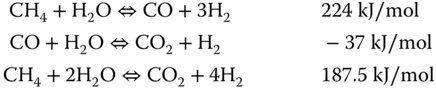
The main reason developers design a SOFC that uses NG is to thermally integrate the reforming and the electrochemical reaction. The NG undergoes a reforming reaction to produce hydrogen and carbon monoxide, CO. The reforming process could be partial oxidation where oxygen is the oxidant. Partial oxidation is exothermic and produces a substantial amount of steam along with CO2. NG decomposes to form solid carbon and hydrogen at elevated temperature (1273–1473 K) according to equation 1.
Studies have shown that regulating the amount of reactant oxygen is an option for controlling the formation of solid carbon (Poppinger and Landes 2001). The reforming process could also be steam reforming, which requires a significant amount of steam and produces relatively more hydrogen per mole of NG reacted. The steam reforming (SR) is well suited for integrated SOFC application since steam produced from the electrochemical reaction can serve as reactant for reforming NG or shifting CO. SR requires a significant amount of thermal energy as show in equation (20.2 since its main reaction is endothermic.
Conversely, SOFC average operating temperature can be (950–1200 K). SOFC developers proposed various way to integrate the reforming process into the SOFC to reduce the amount of energy consumed.
20.1.4 Direct Internal Reforming (DIR) SOFC
Several integration strategies for SOFC have been reviewed (Zhang et al. 2010). One of the design approaches considered is the external reforming SOFC. Here, the reformer is spatially close to the SOFC, and the heat generated for the SOFC is transferred to the reformer through heat integration (Dicks 1998). Contrariwise, in the internal reforming approach the reforming process is within the SOFC. Generally, two design techniques exist for the internal reform of natural gas in SOFC: the Direct internal reforming (DIR) and indirect internal reforming (IIR). In the latter, the stack and the reformer are in thermal contact, and the reformate is fed to the to the adjacent anode. Also, the electrochemical reaction and the reforming reaction are separated. While in the DIR, the NG reform takes place in the anode. The heat generated by the exothermic electrochemical and shift reaction is utilized by the endothermic reforming reactions. Tubular, planar, and monolithic are the predominant geometric configurations of a SOFC (Ahmed and Foger 2000; Klein et al. 2007). Westinghouse (now Siemens‐Westinghouse) developed the tubular SOFC (Kakaç et al. 2007). Planar designs are popular for their compact nature and higher power density. A schematic diagram of a DIR SOFC Cell is shown in Figure 20.3. Due to its high operating temperature, the electrolyte is a nonporous ceramic; Y2O3 stabilized ZrO2 (YSZ). The anode face is made of a porous Nickel/Yttria‐stabilized zirconia (Ni/YSZ) cement, and the nickel serves as a catalyst for the reform reaction. The cathode face is porous Sr‐doped LaMnO3.
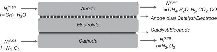
Figure 20.3 Schematic Diagram of a DIR SOFC Cell.
During the operation of the direct internal reforming, natural gas is fed to the anode. The steam from the electrochemical, heat and the nickel catalyst activates the reform reaction producing hydrogen (H2), carbon monoxide (CO), and carbon dioxide (CO2). The shift reaction also utilizes the CO and steam to produce more CO2 and H2. The H2 molecule loses its electron as it adsorbs to the electrode. Air is fed to the cathode. The oxygen in the air gains the electron as it adsorbs to the electrode.
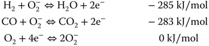
The oxygen ion percolates through the electrolyte to the anode, where it reacts with the hydrogen ion to form steam. One of the challenges of the DIR is the formation of carbon. The decomposition of NG to solid carbon is a thermodynamically favored reaction at the nominal operating conditions at the anode. However, a preferred technique is the addition of steam, since it is a coreactant with NG in the reform reaction. The ratio of steam to methane can be used to regulate the formation of solid carbon (Poppinger and Landes 2001). The steam produced from the electrochemical reaction is used for reforming the NG. Steam is also fed into the system to provide a sufficient amount of steam for the reforming reaction. Mathematical models can be used to estimate the required amount of input steam by analyzing the interactions between various components of the system
20.2 Mathematical Model
The interactions in the SOFC are quite complex, cutting across material sciences, electrochemistry, and transport phenomena etc. This makes the mathematical model a requisite tool for studying the static and dynamic behaviors of SOFC. Several models for SOFC have been developed over the years for various applications. These models range from complex high‐fidelity dynamic, spatial models to data‐driven models. Some researchers have focused on the investigation of the complex interaction in an SOFC using three‐dimensional models (Aguiar et al. 2002; Ferguson et al. 1996; Recknagle et al. 2003; Yakabe et al. 2001). In Bhattacharyya and Rengaswamy (2009) a wide range of dynamic models of SOFC with reformers was reviewed. They categorized the various interactions in the SOFC according to their characteristic time constant and evaluated the models accordingly. In Kakaç et al. (2007) a broader spectrum of SOFC considering the effects of the geometry of the unit on the performance of the system was reviewed. A few researchers have developed models for internal reforming SOFC (Klein et al. 2007). Here we develop a dynamic model describing various fundamental principles of a DIR SOFC. The system adopted is a 12 kW SOFC with the following specifications at nominal operation. The following assumption were made in developing the hypothetical model used here;
- • Ideal gas behavior
- • The pressure correction on the voltage is dependent of hydrogen, oxygen, and steam.
- • The kinetics developed through the experiments conducted by Jianguo Xu and Gilbert Foment (Xu and Froment 1989) is the same for a direct internal reforming SOFC since a nickel‐base catalyst is used in both cases.
- • The anodic and cathodic chambers are well mixed, and the oxidation of hydrogen happens in the anode.
20.2.1 Mass Balance
Anode. The mass balance described here is done according to equations (20.2 and 20.3. The anode takes in NG and a small amount of steam at a molar ratio of 3:1. The NG undergoes a reforming reaction with steam to produce CO and H2. The CO produced is shifted with steam to produce more H2. The H2 produced undergoes an electrochemical reaction with oxygen to produce steam. The steam produced in the electrochemical reaction augments the steam in the inlet stream to make available an abundant steam supply. The material balance in the anode is as follows:
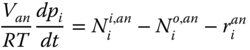
Where Van is the volume of the anode, p is the partial pressure of specie i, R and T are gas constant and temperature respectively, N i is the molar flowrate of specie i, r i is the sum of reactions involving specie I, and i represents all the species in the anode (CO, CO2, H2O, CH4, H2).
Cathode. At the cathode, air flows in, and the oxygen from air adsorbs on the electrode. The adsorbed oxygen seeps through the electrolyte and into the anode as oxygen ions where it reacts with hydrogen ions to form water. The composition of the air is assumed to be 21% oxygen and 79% nitrogen. The material balance in the cathode is given as follows
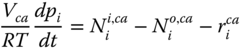
where V ca is the volume of the anode, i represents all the species in the cathode (O2, N2).
20.2.2 Energy Balance
The thermal integration that takes place in the DIR SOFC creates a state where the endothermic reaction is complemented by the exothermic reactions. Here the streams are preheated to 700 °C and are fed at 20 bars (Fernandes and Soares 2006). The partial enthalpies of the inlet and outlet streams of the anode and the cathode make up the first two terms in equation (1.6). The combination of the reaction enthalpies and reacted quantities produces a net heat input from the reaction. This is greatly dependent on the kinetics of the reaction with respect to the equilibrium. About 235 kJ of energy generated for every mole of water produced contributes to power, and some of the heat generated is lost due to radiation.
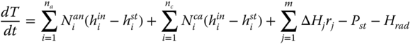
Where ΔH j is the enthalpy of reaction j, h i in and h i st are the enthalpy of the fluid entering and leaving the stack respectively, na and nc are the number of species in the anode and the cathode respectively. P st and H rad are the power of the stack and the heat loss from radiation respectively.
Where A is the surface area of the stack, δ and σ are constants and T surr is the temperature of the surrounding.
20.2.3 Kinetics
The Langmuir Hinshelwood kinetics is used to describe the reforming reaction according to Xu and Froment (1989). The rate expressions for the reaction given by.
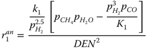
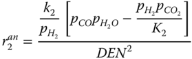
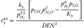
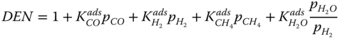
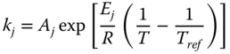
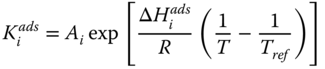
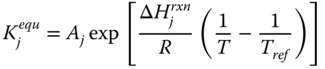
where k j is the rate constant of reaction j; K j is the equilibrium constant of reaction j and K i is the adsorption coefficient of component i.
The kinetic model for the electrochemical reaction is based on a Butler Volmer reaction mechanism in which the rate expressions for reactions is given by
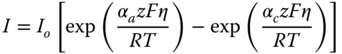
where I is electrode current density, I o exchange current density, z number of electrons involved in the electrode reaction, F Faraday constant, αc cathodic charge transfer coefficient, αa anodic charge transfer coefficient, η activation overpotential
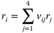
The reaction expressions are applied to the various species as follows.
20.2.4 Electrochemistry
The theoretical or reversible voltage can be derived from the standard Gibbs free energy at any defined temperature. However, the actual cell voltage is less than the theoretical voltage due to overpotentials. Thus, the cell requires more energy than thermodynamically determined. The overpotentials are caused by the activation barriers, V act and resistances to electron, ion, and bulk mass transport, through/to the electrolyte, and charge leaks. The actual cell voltage is the open circuit voltage less the activation overpotential, the concentration overpotential, and the ohmic overpotential (Ziogou et al. 2013; (Gebregergis et al. 2009).
Where V is the actual voltage of the stack, V oc is the open circuit voltage, V act is the activation overpotential, V ohm is the ohmic overpotential, and V conc is the concentration overpotential
The open circuit voltage with pressure change considerations can be expressed as follows.
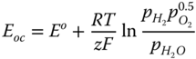
where E o is a temperature‐dependent theoretical/reversible voltage derived from Gibb's free energy.
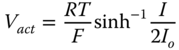
Electrochemical reactions must overcome energy barriers for the reaction to proceed.
The activation loss is derived from the ButlerVolmer equation and given as 20.20:
Io is the exchange current, and it varies with temperature as follows (Gebregergis et al. 2009):
Ohmic overpotentials occur because of the resistance to the flow of ions in the electrolyte and the resistance to the flow of electrons through the electrode materials. The characteristic resistance of a fuel cell as a function of cell temperature is given by (Gebregergis et al. 2009):
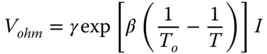
where T0 is the fuel cell reference temperature; T0 = 973 K, γ = 0.2, and β = 2870 K are the constant coefficients of the fuel cell. Concentration overpotentials occur because of the resistance to the transport of material to the triple‐phase boundary for adsorption and subsequent ionization. Concentration over potential V conc is higher when the electrochemical reaction is faster than the flow of material to the triple phase boundary. The limiting current density I L is the current density at which the flow to the triple phase boundary is not sufficient to meet the power demand. V conc related to the current as follows:
20.3 Simulation
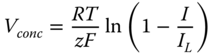
The Model was developed and simulated in gPROMS® (Process Systems Enterprise n.d.). The dynamic model is simulated to investigate the interactions between the manipulated and controlled variables, and for the characterization of the effect of disturbances. The results from the simulations show the transient behavior of the materials and temperature changes. The inlet stream is a mixture of methane and steam at 950 K and a composition ratio of 3:2. The reforming reactions, shift reaction, and the electrochemical reactions occur simultaneously. The model is initialized with some hydrogen in the anode. Steam produced from the electrochemical reaction is used by the reforming and the shift reaction. A polarization curve was derived from the model at constant temperature (950 K) as shown in Figure 20.4. The figure shows how the linear combination of the various overpotentials contributes to the cells' actual voltage. The current produced (flow of produced electrons) in the fuel cell depends mostly on the reaction of hydrogen and oxygen (according to equations (20.2 and 20.16), and the current density is the ratio of the current produced to the total active area of the stack. The active area is a design parameter that is fixed at the design stage. Thus, the polarization curve is used to describe how the voltage changes with the current density. It also shows how the power changes with current density. The limit current density used for the hypothetical model is 2 A/cm2.
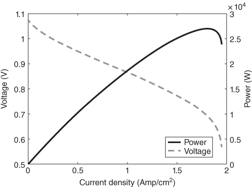
Figure 20.4 Polarization curve.
DIR SOFC is usually subjected to varying power demand; thus it should be robust enough to meet varying power demand. To describe this variability, a power demand profile is used to simulate the dynamic model. The power demand profile is developed by varying current. Figure 20.5 shows the response of the species in the anode and cathode to a change in the current demand, which also corresponds to a power change at constant inlet flow of a mixture of natural gas and steam. Hydrogen and steam have more abrupt response to the variability as would be expected. An increase in the power demand should result in an increased depletion of the hydrogen and an accumulation of steam, which in turn favors the reforming reaction. Generally, the higher the electrochemical reactant pressure, the higher the open circuit voltage. This interaction could be investigated further since the operating conditions favorable for the reforming reaction will increase the amount of hydrogen generated irrespective of the current demand or the rate of the electrochemical reaction. Moreover, if the reforming reaction is more favorable than the electrochemical reaction (probably due to the current demand), the temperature of the system might start decreasing and will tend to slow down the reforming reaction.
Figure 20.5 Transient change in mole fraction with change in power demand.
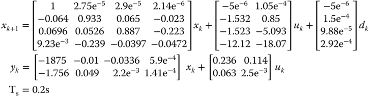
One of the major challenges of fuel cells is the voltage fluctuations that accompany a change in current or power demand. This phenomenon occurs as a result of multiple time constants in the various fuel cell interactions. Figure 20.6 shows how voltage changes with current or power change. An ideal process operation would be to have the voltage remain relatively constant with slight perturbation of the current. A controller can be used to regulate the voltage to a set‐point, for slight change in the power demand. A controller, however, cannot be used to effectively circumvent the mass transport limitation of a fuel. The fuel is usually integrated with a battery or a capacitor to make up for its limitations. The thermal coupling of the reforming, the shift and the electrochemical reaction in a direct internal reforming, is a development that needs to be studied critically. It has the potential to greatly improve the energy efficiency and cost of an SOFC. This combination of exothermic and endothermic reactions at varying reaction rates (or time constants) has a significant impact on the temperature of the system. Generally, fuel cell control designs are intended to regulate disturbances caused by changing current demand, track load demand, comply with safety or operational constraints, and improve efficiency. The control developed here will attempt to maintain a voltage set‐point while constraining the temperature of the system within a bound.
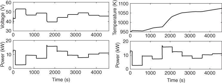
Figure 20.6 Transient change in Voltage and Temperature with change in power demand.
20.4 Multiparametric Model Predictive Control (mpMPC)
An advanced process control framework is used to design a controller for the DIR SOFC. The PARametric Optimization and Control (PAROC) framework is a framework that enables the representation and solution of demanding model‐based operational optimization and control problems following an integrated procedure featuring high‐fidelity modeling, approximation techniques, and optimization‐based strategies, including multi‐parametric programming (Pistikopoulos et al. 2015). The PAROC framework can adapt to several classes of problems through its prototype software platform. PAROC has been used to design controllers for PEMFC (Ziogou et al. 2013); however, the dynamic of an IR SOFC is different and more complex from a control standpoint.
20.4.1 PAROC Framework
The first step of the PAROC framework is to develop a high‐fidelity model that correctly describes the various aspects of the system. The dynamic model described above can easily be adapted for controller design. However, the model has some complex nonlinear expressions that make it difficult to be directly adapted for control studies. Consequently, it is necessary to simplify the representation of the model without compromising its accuracy. PSEs gPROMS Model Builder software allows direct communication with MATLAB through gO:MATLAB for further analysis. The simplification of the model is carried out in MATLAB.
20.4.1.1 Linear Model Approximation
A series of simulations of the dynamic model for different input is used to construct a meaningful linear state‐space model of the process using statistical methods. The inputs are the inlet flowrate for the anode and the cathode while we measure voltage current and temperature. The current is treated as a disturbance. One of the most widely applied tools within this area is the N4SID algorithm within the System Identification Toolbox from MATLAB. The sampling time for the input‐output data is 200ms. A discrete linear state space model is obtained from the input‐output data. The mathematical expression of the SS model is of the form of eq. 20.24:
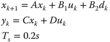
The SS model generated have 4 identified states (x k ), 2 outputs (y k ), 2 inputs (u k ) and 1 disturbance (d k ). The state space model is given in eq. 20.25.
The approximate model was compared to the original nonlinear model in Figure 20.8. For brevity, only one input (anode inlet flowrate) and output (voltage) are shown here, however the inlet flow of the cathode was varied too, and the temperature fitting curve was obtained. The temperature has an R2 value of 99% while that of the voltage (Figure 20.7) is 79%.
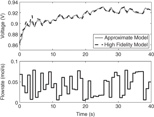
Figure 20.7 Comparison of linear SS model and the original model.
There are eight states in the original dynamic model, however; for purposes of simplification, the linear discrete state‐space model consists of four states. Not only are the states reduced, but their physical meaning is lost during the system identification process. To maintain the accuracy of the original complex dynamic model, a state observer is employed to estimate the state of the system using the linear model. The Kalman filter is a type of observer that uses a least square estimation approach to characterize the current state of a dynamic system based on the influence of past measurement. Its prime feature is the iterative propagation of the noise measurement risk. For further reading on the Kalman Filter used in this work see Yu et al. (2005).
20.4.1.2 mpMPC Controller Design
The generic expression of the model predictive control is given in eq. 20.26.
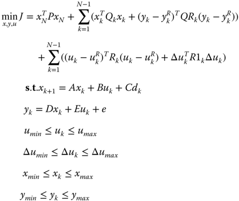
where x k are the state variables; u k and u R k are the control variables and their respective set‐points; Δu k denotes the difference between two consecutive control actions; y k and y R k are the outputs and their respective set‐points; d k are the measured disturbances; Q k , R k , R1 k, and QR k are the corresponding weights in the quadratic objective function; P is the stabilizing term derived from the Riccatti equation for discrete systems; N and M are the output horizon and control horizon, respectively; k is the time step; A, B, C, D, and E are the matrices of the discrete linear state‐space model; and e denotes the mismatch between the actual system output and the predicted output at initial time.
This quadratic problem in eq. 20.26 can be reformulated into a multiparametric quadratic programming problem (mp‐QP) (Bemporad et al. 2002). The uncertain parameters are denoted by θ, and they include the initial states x 0 , the set‐points y R k , previous control actions u −1 for evaluating Δu k , and the disturbances d k . The mp‐QP is given as follows:
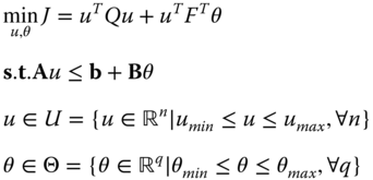
where u is a vector that consists of M control actions, n and q are the size of the control and parameter vector respectively, and consequently the size of the parametric solution and parametric space of the problem.
The multi‐parametric model predictive controller problem is formulated and solved using the POP toolbox in MATLAB. The objective function of the mpMPC is to meet the electrical power demand at a constant voltage amid the current charge and to maintain the temperature below 1500 K. The optimal control action is generated as a map of solutions and as an affine function of the aforementioned parameters. Thus, at every time step a set of parameters, realized from measurements and estimations, is used as inputs to evaluate the affine function generated from the mp‐QP solution. Table 20.2 shows the mpMPC design specification and bounds on various variables. The bounds on the output variable u k and y k have been set according to the complex dynamic model simulation results. However, the bounds on x k are exaggerated since the states of the linear state space model do not necessarily represent the state of the original system. The choice of bounds on x k also reflects the usage of an unconstrained state approximation technique: i.e., the Kalman filter. Alternatively, constrained state estimation techniques such as the (multi‐parametric) Moving Horizon Estimator ((mp‐)MHE) can be utilized (Darby and Nikolaou 2007; Voelker et al. 2013; Nascu et al. 2014; Pistikopoulos et al. 2015). The tuning of the controller is presented in section 20.5.
Table 20.2 Weight tuning for the mpMPC of the DIR SOFC unit.
| mpMPC design parameters | Value |
| N | 5 |
| M | 2 |
| QR k , ∀ k ∈ {1, …, N } | 100 |
| R 1 k , ∀ k ∈ {1, …, M } |
|
| x min | −500[1 1 1 1] |
| x max | 500[1 1 1 1] |
| u min | [0.002 0.004] |
| u max | [0.1 0.1] |
| y max | [2000 1.2] |
| y min | [900 0.1] |
| Δ u min | −[0.05 0.05] |
| Δ u max | [0.05 0.05] |
20.5 Closed‐Loop Validation and Results
The controller is validated by closing the loop on the controller design. The controller is used on the original complex dynamic model to check if the controller can actually control the system from which it was designed. The validation process involves calculating the control action from the realized parameters and the mp‐QP generated affine function. The control action calculated is used as input to the original dynamic model. The output Voltage is measured to and compared with the set‐point value as shown in Figure 20.8. This is enabled through gO:MATLAB, an application that links the gPROMS with MATLAB. Figure 20.8 also shows how the flow of NG in the anode and flow of air in the anode changes with changes in current. The power demand is varied by changing the current. Figure 20.9 shows how the controller‐enabled DIR SOFC tracks the power demand (product of the current and voltage). The controller follows the set‐point effectively. The temperature is maintained below the bound as also shown in Figure 20.9.
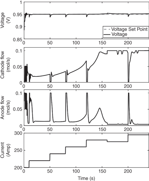
Figure 20.8 Closed‐loop validation results of the mpMPC controller showing the voltage set‐point tracking (top) the anode (natural gas and steam) and cathode (oxygen) flowrate (middle) and the current profile (bottom).
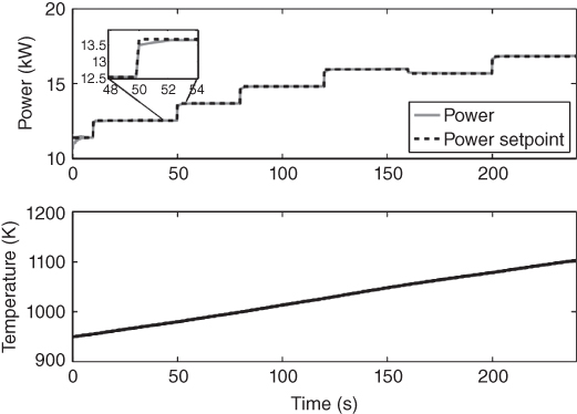
Figure 20.9 Closed‐loop validation results showing the power set‐point tracking and the temperature.
20.6 Conclusion
We demonstrated the use of a natural‐gas‐based DIR SOFC for distributed electricity generation. In addition, we developed a complex dynamic model of a hypothetical DIR SOFC to describe the various interactions between the reforming reaction, the transport phenomenon, and the electrochemical reaction.
Using the PAROC framework, we designed a multi‐parametric model Predictive controller for regulating the voltage of the power generated by the DIR SOFC. The controller was validated with the complex dynamic model. In future work, we intend to explore how the DIR SOFC compares with other intensified distributed electricity generation units. An economic analysis of the DIR SOFC and other auxiliary unit that make up the balance of plant will be essential for benchmarking it with other technologies.
References
- Aguiar P, Chadwick D, Kershenbaum L., 2002. Modelling of an indirect internal reforming solid oxide fuel cell. Chemical Engineering Science, 57(10): 1665–1677.
- Ahmed K, Foger K. 2000. Kinetics of internal steam reforming of methane on Ni/YSZ‐based anodes for solid oxide fuel cells. Catalysis Today, 63(2): 479–487.
- Al‐Fattah SM, Startzman RA. Forecasting world natural gas supply. Society of Petroleum Engineers. SPE/CERI Gas Technology Symposium, 3–5 April, Calgary, Alberta, Canada.
- Battelle 2014. Manufacturing cost analysis of 1 KW and 5 KW Solid oxide fuel cell (SOFC) for auxillary power applications. Available from: https://www.energy.gov/eere/fuelcells/downloads/manufacturing‐cost‐analysis‐1‐kw‐and‐5‐kw‐solid‐oxide‐fuel‐cell‐sofc.
- Bemporad A et al. 2002. The explicit linear quadratic regulator for constrained systems. Automatica, 38(1): 3–20.
- Bhattacharyya D, Rengaswamy R. 2009. A review of solid oxide fuel cell (SOFC) dynamic models. Ind. Eng Chem Res, 48(13): 6068–6086.
- Burnham A et al. 2011. Life‐cycle greenhouse gas emissions of shale gas, natural gas, coal, and petroleum. Environ Sci Technol, 46(2): 619–627.
- Darby ML, Nikolaou M. 2007. A parametric programming approach to moving‐horizon state estimation. Automatica, 43(5): 885–891.
- Diangelakis NA, Pistikopoulos EN. 2017. A multi‐scale energy systems engineering approach to residential combined heat and power systems. Comput Chem Engg, 102, p.128–138.
- Dicks AL. 1998. Advances in catalysts for internal reforming in high temperature fuel cells. J Power Sources, 71(1): 111–122.
- Ferguson JR, Fiard JM. Herbin R., 1996. Three‐dimensional numerical simulation for various geometries of solid oxide fuel cells. J Power Sources, 58(2): 109–122.
- Fernandes FAN, Soares AB. 2006. Methane steam reforming modeling in a palladium membrane reactor. Fuel, 85 (4): 569–573.
- Gebregergis A, et al., 2009. Solid oxide fuel cell modeling. IEEE Transactions Indus Electron, 56(1): 139–148.
- Hawkes A, Leach M. 2005. Solid oxide fuel cell systems for residential micro‐combined heat and power in the UK: Key economic drivers. J Power Sources, 149, p.72–83.
- Hore‐Lacy I. 2006. Nuclear energy in the 21st century. Elsevier. eBook ISBN: 9780080497532.
- Jin W et al. 2004. Low cost fuel cell converter system for residential power generation. IEEE Trans Power Electron, 19 (5): 1315–1322.
- Kakaç S, Pramuanjaroenkij A, Zhou XY. 2007. A review of numerical modeling of solid oxide fuel cells. Int. J Hydrogen Energ, 32(7): 761–786. Available from: http://dx.doi.org/10.1016/j.ijhydene.2016.02.089.
- Klein JM, et al. 2007. Modeling of a SOFC fuelled by methane: from direct internal reforming to gradual internal reforming. Chem Engg Sci, 62 (6): 1636–1649.
- Lasseter RH. 2007. Microgrids and distributed generation. J Energ Engg, 133(3): 144–149.
- Mohr SH, Evans GM. 2011. Long term forecasting of natural gas production. Energ Policy, 39 (9): 5550–5560.
- Nascu I et al., 2014. Simultaneous multi‐parametric model predictive control and state estimation with application to distillation column and intravenous anaesthesia. In: 24th European Symposium on Computer Aided Process Engineering. Computer Aided Chemical Engineering, Budapest, Hungary: Elsevier, pp. 541–546.
- Pistikopoulos EN, et al., 2015. PAROC An integrated framework and software platform for the optimisation and advanced model‐based control of process systems. Chem Engg Sci, 136: pp.115–138.
- Poppinger M, and Landes H. 2001. Aspects of the internal reforming of methane in solid oxide fuel cells. Ionics, 7(1): 7–15.
- Process Systems Enterprise. gPROMS. Available from: www.psenterprise.com/gproms.
- Recknagle KP et al, 2003. Three‐dimensional thermo‐fluid electrochemical modeling of planar SOFC stacks. J Power Sources, 113 (1): 109–114.
- Riensche E, Stimming U, Unverzagt G. 1998. Optimization of a 200 kW SOFC cogeneration power plant. J Power Sources, 73(2): 251–256.
- U.S. Energy Information Administration and U.S. Department of Energy. 2011. Ann Energ Outlook 2011 with Projections to 2035, Available from: http://www.eia.gov/forecasts/aeo/pdf/0383(2011).pdf.
- U.S. EIA, 2016. Carbon Dioxide Emissions Coefficients, U.S. Energy Information Adminstration. Available from: https://www.eia.gov/environment/emissions/co2_vol_mass.cfm.
- U.S. NETL. 2013. Modern shale gas development in the united states : an update. U.S. Department of Energy, 2013 (September): 1–79.
- Voelker A, Kouramas K, Pistikopoulos EN. 2013. Moving horizon estimation: error dynamics and bounding error sets for robust control. Automatica, 49(4): 943–948.
- Xu J, Froment GF. 1989. Methane steam reforming, methanation and water‐gas shift: I. Intrinsic kinetics. AI Ch E Journal, 35(1): 88–96.
- Yakabe H, et al., 2001. 3‐D model calculation for planar SOFC. J Power Sources, 102(1): 144–154.
- Zhang X, et al., 2010. A review of integration strategies for solid oxide fuel cells. J Power Sources, 195(3): 685–702.
- Ziogou C, et al., 2013. Empowering the performance of advanced NMPC by multiparametric programming—an application to a pem fuel cell system. Indus Engg Chem Res, 52(13): 4863–4873.