
2
Air and Maritime Transport
At its height in the 2nd Century, the Roman Empire extended over the entire Mediterranean region. Land and sea routes ensured the domination of Rome, which derived its wealth from the exploitation of the resources of the territories it controlled. Supported in particular by intercontinental means of transport, the globalization of trade, initiated in antiquity, intensified in the 20th Century to a level probably never seen before in human history (Figure 2.1).

Figure 2.1. To which countries does the world export? (source: Observatory for Economic Complexity/www.atlas.media.mit.edu). For a color version of this figure, see www.iste.co.uk/sigrist/simulation2.zip
COMMENT ON FIGURE 2.1.– In 2017, world trade represented $16.3 trillion, with exportations to Europe accounting for 38% of the total amount, to Asia 37% and to North America 18%. The United States, China and Germany were the top three importing countries. Nearly 90% of world trade was carried out by sea, with 9.1 billion tons of goods transported on ships sailing across the oceans.
2.1. The long march of globalization
The current globalization is the result of a period of intensive exploration of the Earth undertaken by Europeans between the 15th and 17th Centuries. European expeditions helped to map the planet and create maritime trade routes with Africa, America, Asia and Oceania. In 1492, the Italian navigator Christopher Columbus (1451–1506), financed by the Spanish monarchy, crossed the Atlantic Ocean and reached a “New World”: America, named after the navigator Amerigo Vespucci (1454–1512), who understood that the lands discovered by Columbus were indeed those of a new continent. In 1498, the Portuguese navigator Vasco da Gama (1469–1524) led an expedition establishing the first maritime link with India by sailing around Africa. Explorations to the west and east continued with the Portuguese Ferdinand Magellan (1480–1521) who performed the first circumnavigation of the Earth in 1522. This first globalization is leading to some of the most significant ecological, agricultural and cultural changes in history. European exploration ended in the 20th Century, when all the land areas were mapped.
At the end of the 18th Century, when the shipbuilding techniques of the time were recorded in works that reflected the latest knowledge in the field (Figure 2.2), a technological revolution began: humans realized Icarus’ ancient dream!

Figure 2.2. Taken from the work of Édouard-Thomas de Burgues, Count of Missiessy, Stevedoring of Vessels, published by order of the King, Under the Ministry of Mr. Le Comte de la Luzerne, Minister & Secretary of State, having the Department of Marine & Colonies. In Paris, from the Imprimerie Royale, 1789
(source: personal collection).
In 1783, the French inventors Joseph-Michel and Jacques-Étienne Montgolfier (1740–1810 and 1745–1799) developed the first hot-air balloon capable of carrying a load through the air. The first flight demonstration of the hot air balloon took place in Versailles in September 1783 in front of King Louis XVI. A sheep, a duck and a rooster were the guinea pigs on this balloon trip1. The first balloon flight piloted by humans dates back to November 1783: the French scientists Jean-François Pilâtre de Rozier (1754–1785) and François-Laurent d’Arlandes (1742–1809) became the first two aeronauts in history. Despite its imposing mass, nearly a ton, the balloon designed by the Montgolfier brothers took off from the Château de la Muette, on the outskirts of Paris. It landed in the middle of the city some 25 min later, after reaching an assumed maximum altitude of 1,000 m and traveling about 10 km.
Aeronautics then developed because of the work of the British engineer George Cayley (1773–1857) who understood the principles of aerodynamics and designed the first shape of an aircraft. The invention of this word is attributed to Clément Ader (1841–1925), a French engineer known at the time for his work on the telephone. In October 1890, he succeeded in making the first flight of an aeroplane carrying its engine and pilot. “Éole”, his aeroplane, was inspired by the flight of storks and bats. It was powered by a propeller driven by a twin-cylinder steam engine. The German engineer Otto Lilienthal (1848–1896) then carried out numerous flight experiments on small gliders and understood the importance of designing curved wings. The Americans Orville and Wilbur Wright (1871–1948 and 1867–1912) designed small planes on which they perfected their flight control, going from about 10 seconds and a few meters for Orville in 1903 to more than 2 hours and several hundred kilometers for Wilbur in 1908. In France, the United States, England and Denmark, the public was fascinated by the exploits of the pioneers of aviation. The first continental and maritime crossings followed one another: the French Louis Blériot (1872–1936) crossed the English Channel in 1909, the American Charles Lindbergh (1902–1974) the Atlantic in 1927.
The First and Second World Wars accelerated the development of aeronautical and naval technology. Aircraft were equipped with weapons and contributed alongside submarines to intelligence, convoying and offensives. The aircraft carrier allowed squadrons to be projected beyond the land and the naval air forces played a decisive role in the Second World War [ANA 62, BAY 01, SMI 76].
After 1945, the military and civil construction industries developed jointly and today, air and sea transport evidence record traffic (Figure 2.3): nearly 50,000 ships carry 90% of the goods traded every year worldwide, while some 100,000 flights carry more than 3.5 billion passengers.
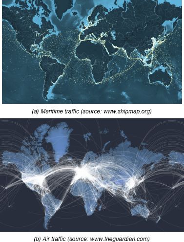
Figure 2.3. Visualization of maritime and air traffic. For a color version of this figure, see www.iste.co.uk/sigrist/simulation2.zip
Aircraft and ships also reach new transport capacities:
- – In 2005, Airbus completed the first flight of the A380, the largest civil passenger aircraft in service. Four years later, Air France operated the aircraft’s first commercial flight between Paris and New York [MOL 09]. Powered by four engines and equipped with a double deck, the A380 can carry up to 850 passengers at nearly 1,000 km/h over a distance of 15,000 km2;
- – In 2018, the French shipping company CMA-CGM welcomed the “Saint Exupéry” [STU 18], a freight ship built by Hanjin Heavy Industries and Construction in the Philippines, into its fleet. It is 400 m long, it can reach more than 20 knots and carries a cargo of 20,600 TEU (arranged end-to-end, the containers it ships form a chain of more than 123 km)3.
There are many issues involved in the design of ships and aircraft. It is a question of manufacturers guaranteeing ever-increasing performance – in terms of safety, speed, silence, service life, energy consumption, comfort or environmental impact – posing ever-increasing innovation challenges for engineers.
Without claiming to be exhaustive, as the subjects are so varied, this chapter proposes some examples where numerical simulation accompanies engineering studies in shipbuilding and aeronautics and where it contributes to improving performance.
2.2. Going digital!
The America’s Cup is one of the oldest sailing yacht competitions. Since the end of the 19th Century, it has seen international teams compete against each other. Traditionally raced on monohulls, it also gives space to multihulls. Catamarans that are lighter and lighter, with thin lines and dynamic hulls, literally float above the water. Saving themselves from friction, much more significant on water than in air, they reach ever higher speeds! This innovation was partly made possible by simulations in fluid mechanics (Box 2.1), of which the Swiss physicist and mathematician Daniel Bernoulli (1700–1782) was one of the pioneers. In particular, he understood that, in a fluid flow, acceleration occurs simultaneously with the decrease in pressure and proposed an equation to account for this observation. This physical property is used by engineers to design aircraft wings, propellers, wind turbines or hydrofoils for the catamarans used in offshore racing.
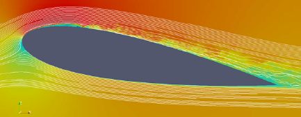
Figure 2.4. Flow calculation around a lifting profile (source: Naval Group). For a color version of this figure, see www.iste.co.uk/sigrist/simulation2.zip
COMMENT ON FIGURE 2.4.– The shape of the foils allows a flow of water or air to be separated at the leading edge, before joining at the trailing edge. The fluid flowing on the upper part of the foil, the “suction side”, travels a greater distance than the fluid flowing on its lower surface, the “pressure side”. According to the law established by Bernoulli, the accelerated flow on the upper surface exerts a lower pressure on the profile than that of the slowed flow under the lower surface. This pressure difference generates a force on the foil: hydrodynamic lift. The lift flow calculation shown in the figure indicates how the water flow flows around the hydrofoil (white lines). It also highlights the regions of overpressure (low-velocity regions in green and blue) and depression (high-velocity region in red) responsible for the lift.
The lift created by the movement of air or water allows an aircraft to fly, a propeller or sail to propel a ship, or a wind turbine to recover wind energy. With a proper curvature and an adequate inclination of the foil on the hull, the lift exceeds the weight of the ship and it can almost fly. The challenge is then to optimize the shape of the foil, in order to achieve the best possible separation of the flows at the leading edge, to ensure their reattachment at the trailing edge and to limit the pressure fluctuations generated by turbulence phenomena in the flow. An art, permitted for more than two centuries by the Bernoulli equation.
Useful for understanding fluid physics, however, this equation is too simple to help engineers in their design tasks. Nowadays, they use more complete models that accurately represent fluid dynamics. To this end, they resort to the power of computers to represent hydrodynamics and understand it by means of a calculation.
Naval designers and constructors are increasingly using numerical simulation to propose new shapes or materials for hulls, sails or any important part of the sailboat. However, it is necessary to choose the most efficient ones so as to achieve the expected performance in the race: material resistance, flow understanding, hydrodynamic, and aerodynamic performance, as with these flying yachts. These innovations pave the way for other applications in naval architecture and the computational techniques that can assist designers are varied. They use generalist tools, such as tools more specific to the sail design profession, for example (Figure 2.5).

Figure 2.5. Simulation of the aerodynamics of a sail
(source: image owned by TotalSim/www.totalsimulation.co.uk)
The sailboat’s speed prediction is based on different calculation techniques. Starting from a given architecture (rigging, platform, appendages, etc.), it is a question of finding the best possible adjustments to the sailboat (heading, speed, etc.) in order to achieve the highest speed under the assumed sea conditions (in particular the speed of sea and air currents).
The simulation is based on an experiment matrix defining the different possible configurations and the associated calculation points. The adjustment of a foil or appendage explores a thousand configurations. The data are calculated in about 10 days. They are then analyzed using advanced algorithmic techniques to determine an optimal setting. Simulation makes it possible to identify general trends that are useful to designers and contribute to a sensitivity analysis. It is a matter of sequencing the architectural parameters that have the greatest influence on a given ship’s behavior.
Benjamin Muyl, consulting engineer, indicates the direction of the next innovations in this field:
“Tomorrow, the simulations will also take on the wide-open sea: from static (where sea and wind conditions are frozen), the simulations will become dynamic. The aim will be to propose behavioral models that evolve over time. The applications envisaged are numerous, from the crew training simulator to optimal control. The latter allows better adjustments in very critical race phases, such as the passage of buoys, where the slightest tactical error can be difficult to catch up!”
What is the next horizon for the simulations? Real-time models! Integrated on board ships, they assist the sailors involved in the race or assist the skippers in their choice of settings at sea.
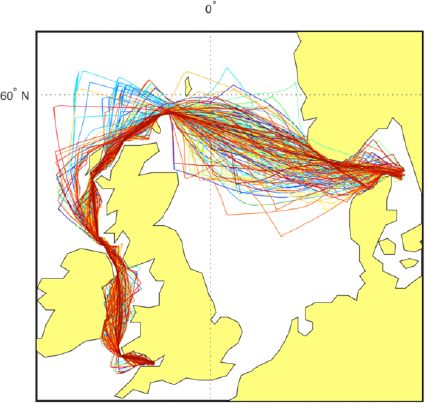
Figure 2.6. Simulation of possible routes for an offshore race (image made using Neptune code, routing software developed by Xavier Pillons; source: BMD/www. www.bmuyl.com). For a color version of this figure, see www.iste.co.uk/sigrist/simulation2.zip
Engineers anticipate a convergence between scientific computing and new techniques, such as data learning. Everything remains to be imagined and built and it is a new direction that simulation is taking in many other fields. As in ocean racing, the road choices for the development of new generation simulations are varied and carry their share of uncertainty. Chance is part of ship racing, and fortunately has little to do with technology! So may the best (and luckiest) skipper win the next race… with or without the invisible help of algorithms.
2.3. Optimum design and production
2.3.1. Lightening the structures
Combining properties of both rigidity and lightness, composites are increasingly used in many industrial sectors, particularly in aircraft, space, automotive and shipbuilding. These materials contribute to the structural weight reduction objectives set by manufacturers in order to reduce operating costs – in particular those of fuel consumption. Pascal Casari, an expert in composite materials at the University of Nantes, tells us:
“Aeronautics is the industrial sector that most systematically uses composite materials. Long before the birth of large aircrafts, such as the A380, these materials were chosen in the design of aerobatic planes, for which weight gain is crucial! Other sectors have then gradually adopted them: the automobile and shipbuilding industries nowadays use composites to design many parts, some of which contribute to essential functions, such as structural integrity”.
A composite is a heterogeneous material, obtained by assembling different components with complementary properties. Generally made of fibers, the reinforcement of the composite ensures its mechanical strength, when the matrix, most often a thermoplastic or thermosetting resin, allows the cohesion of the structure and the transmission of forces to the reinforcement (Figure 2.18). The structure is then organized into laminated folds that constitute thin structures particularly suitable for high-performance applications.

Figure 2.18. Example of a composite material: a multilayer (source: www.commons.wikimedia.org). For a color version of this figure, see www.iste.co.uk/sigrist/simulation2.zip
“Composite modeling poses many challenges for researchers and engineers in mechanics and materials science. Obtained by various processes (weaving of fibers, injection of resin, etc.), they are produced by injection or forming and may contain defects: they are thus media with ‘inhomogeneous’ (they vary from one point to another of the part) and ‘anisotropic’ (they depend on the direction of stress) mechanical properties. Thus, the mechanical strength criteria valid for homogeneous and isotropic materials, such as metallic materials, are generally too conservative for composites”.
After decades of using criteria based on “material strength” [TSA 08], mechanical engineers are now developing criteria that are better able to represent the damage mechanisms of composites.
“To that end, it is thus necessary to better calculate the internal cracking at the folds or at the interface between the folds, leading to the wear mechanisms called ‘delamination’ and to model the effects of the environment (temperature or humidity) on their ageing”.
Composites simulation is used by engineers with two main objectives, explains Christophe Binétruy, modeling expert at the École Centrale de Nantes:
“Numerical modeling makes it possible to carry out real ‘virtual tests’ in order to determine by calculation the mechanical properties of materials, such as their rigidity or their resistance to different thermomechanical stresses. Calculations give engineers the ability to ‘digitally’ design a material, which will then be developed to obtain the desired characteristics for a given product or use. Simulations are also used to optimize manufacturing processes: designing a mold, dimensioning a tool or anticipating the formation of defects are among the research objectives nowadays”.
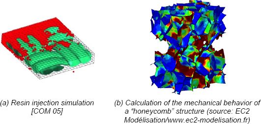
Figure 2.19. Numerical simulation for composites: manufacturing processes and mechanical properties. For a color version of this figure, see www.iste.co.uk/sigrist/simulation2.zip
COMMENT ON FIGURE 2.19.– Numerical simulation helps to understand the mechanisms of impregnation of a fibrous network with a resin (left). Starting from a known arrangement of fibers, characterized experimentally by means of imaging tools, it is possible to predict by calculation how the fluid occupies the volume at its disposal, as a function of its injection rate and rheological properties. The simulation is based, for example, on highly viscous flow equations, described by the “Stokes model”, or on flows in porous media, described by the “Darcy model”. While the calculation presented here uses the SPHparticle method [MON 88], other numerical methods, such as finite elements, are also effective for performing this type of simulation. The models can be refined to take into account the chemical transformations of the resin during cooling and solidification, which are described by thermal and thermodynamic equations. The overall mechanical properties of a composite material can also be calculated. The figure shown on the right details a calculation of the mechanical strength of a honeycomb composite structure. This type of simulation makes it possible to predict the characteristics of the part to be built with this material – the remaining numerical calculations to scale one, for large objects, is still not very accessible due to modeling costs and calculation times. Simulations require real expertise in data specification, interpretation of results and overall calculation management: it is generally performed by experts in the field.
“Calculation to the scale of the material is still a necessary step: with composites, it is difficult to deduce the characteristics of a structure from those of a tested specimen. In addition, gathering the geometric and physical properties of composites remains very tedious: these can be obtained reliably at the cost of expensive tests. Since the latter also present a very high variability, simulation appears to be an effective tool for quickly assessing the consequences of this variability on the properties of the material”.
With composites, numerical simulation contributes to the development of materials science. Enabling the design of parts with the qualities expected for industrial uses, it requires us to think at the same time about the product to be manufactured and the desired characteristics of the material which it will be made of. Beyond the product and the material, it is also developing in order to understand and optimize manufacturing processes.
2.3.2. Mastering processes
In the shipbuilding industry, as in other mechanical engineering industries, welding is a widespread operation (Figure 2.20).
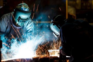
Figure 2.20. Welding operation
(source: www123rf.com/Praphan Jampala)
For instance, a frigate hull is made of metal panels on which stiffeners are welded to ensure its resistance – to difficult sea conditions as well as to different types of attacks (explosions and impacts). Tens of thousands of hours of welding time are required to build a ship. The process uses a wide variety of techniques and sometimes welders work under difficult conditions, for example in areas of the ship where access is difficult. Mastering welding techniques requires long experience that must sometimes be adapted to a new construction.
The metal is heated at the weld point and it deforms: over large dimensions, this residual deformation can even be observed with the naked eye. Under the effect of the heat imposed at the time of welding, the metal is also transformed. It is under tension, like skin that heals. The residual stresses should be as low as possible so as not to reduce the overall strength of the ship hull. Deformations or residual stresses are sometimes too high: this non-quality of production can weigh heavily on the production costs of a series of vessels, partly because straightening deformed shells or repairing some welding areas is time consuming.
Florent Bridier, numerical simulation expert at Naval Group, explains how modeling can be used to understand welding:
“Numerical simulation of welding helps to optimize the process (the sequencing of the passes, or the pre- or post-heating phases), or to validate the repair techniques. At stake: avoiding thousands of extra hours of work at the shipyards, which justifies assessing the value of this technique in order to modify and optimize certain welding operations”.
Welders and researchers share their knowledge of the process and its abstract modeling: their practices are mutually beneficial. The simulation may be based on a so-called “multi-physics” model to account for the complexity of the phenomena involved in welding. In order to obtain the most accurate simulations possible, it is necessary to describe:
- – the supply of heat, and possibly of material, by the welding process used, as well as its diffusion in the concerned area. It can be carried out in several steps, which the simulation will take into account;
- – the transformations of the matter undergoing these thermal effects. The structure of metal crystals is influenced by temperature and in turn changes the mechanical properties of the material (such as its strength, ability to absorb or diffuse heat, etc.);
- – the mechanical behavior of the metal in the area where it melts, as well as the deformations and stresses it undergoes.
These physical phenomena are coupled in the sense that one influences the other and vice versa (Figure 2.21). A direct simulation of welding quickly becomes very costly in terms of modeling and calculation time, especially for real configurations. Instead, it is used on simple geometries, representing a specific area of a ship. The complete multiphysical calculation performed on a T-joint shows the temperature distribution in the joint and reports the formation of the weld seam (Figure 2.22). It provides accurate data on the operation. These are used on a simpler model at the scale of a hull panel. The simulation allows us to choose a welding sequence that limits residual deformations. The use of such calculation is twofold:
- – assist welders in adjusting process parameters (e.g. size and intensity of heat source);
- – produce a digital database for different shapes of welded joints, according to different processes used. These data are then used in simplified models, allowing calculations at the scale of the welded panels.
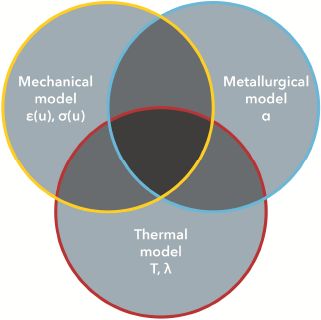
Figure 2.21. The thermal, mechanical and metallurgical phenomena involved in welding are coupled and simulated together
COMMENT ON FIGURE 2.21.– The temperature (T), thermal conductivity (λ), phases (α) and deformations/stresses (ε(u), σ(u)) in the metal are the physical quantities to be calculated. They depend on each other: the accuracy of the model depends on the representation of all these effects in the calculation.
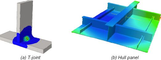
Figure 2.22. Numerical simulation of welding (source: Naval Group). For a color version of this figure, see www.iste.co.uk/sigrist/simulation2.zip
To be accurate and reliable, the simulation uses the metal characteristic data and how it changes with temperature or in the crystal state. These data, obtained at the cost of expensive experimental campaigns, constitute a real asset for the companies or laboratories that produce them.
2.3.3. Producing in the digital age
2.3.3.1. Factory of the future
The Brazilian photographer Sebastião Salgado [WEN 14] published at the end of the 1990s a book entitled La main de l’homme (meaning ‘the hand of man’), in which one can feel the gaze of the economist, his youth training. It is a look driven by the need to carry out an inventory of the work places in the world. At a time when the digital economy was emerging, with the Internet for the general public in its infancy, he had the intuition that work, especially manual work, was not disappearing, and he told it in its diversity [SAL 98]: net and boat fishing in the Mediterranean Sea, tunnel construction under the Channel, cultivation and harvesting of sugar cane and coffee in tropical areas, ship dismantling in India, textile manufacturing in sweat shops in Asia, fire-fighting on oil wells in Iraq. Humans and their bodies, very often mistreated by exhausting work, from which they derive their livelihoods, suffering as well as dignity. Some of his photographs, showing the work of workers in factories or on construction sites, testify to some of the most trying conditions faced by humans, which, in the Western world, are sometimes entrusted to machines. The human hand is imitated by robots performing various tasks that are increasingly complex, fast and precise.
In the industrial sector, robots perform repetitive tasks, their use being adapted to the productivity and quality requirements of mass production. However, human know-how remains a guarantee of quality: delicate operations requiring precise execution are, in many cases, carried out by manual labor. Some of the engineers’ research concerning the factory of tomorrow [KOR 16, TAT 18] aims to relieve humans in the performance of delicate and difficult tasks when they are carried out over time. A part of the robotic developments concerns collaborative robots, capable of adapting to human gestures by anticipating and accompanying them (Figure 2.25).
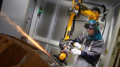
Figure 2.25. Collaborative robot
(source: © RB3D/www.rb3d.com)
Jean-Noël Patillon, scientific advisor of the List research institute at the CEA (one of France’s pioneering centers in this field), explains what cobots are:
“For many tasks performed with tools, human know-how is irreplaceable. ‘Cobotic’ researches aim to develop systems that adapt to humans. They make it possible to build systems capable of learning in real time about human actions. Like models made in biomechanics, cobotic engineers develop ‘digital twins’. An abstract representation as close as possible to the human being. The models specific to each operator are coupled with automatic learning techniques operating in real time and making it possible for the human and robot to collaborate”.
The digital twin, the numerical modeling of a physical process, is no longer reserved for mechanical systems: body modeling also serves humans. It makes it possible to support them and, as we will see in the case of biomechanics, to heal them (Chapter 6). Virtual and augmented reality also complete the range of digital techniques shaping the factory of the future:
– virtual reality refers to a set of techniques and systems that give humans the feeling of entering a universe (Figure 2.26). Virtual reality gives us the possibility to perform in real time a certain number of actions defined by one or more computer programs and to experience a certain number of sensations (auditory, visual or haptic, for example);
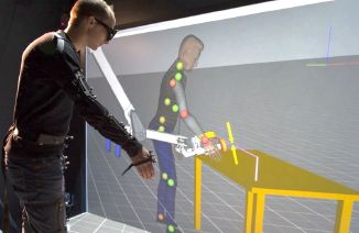
Figure 2.26. Ergonomics demonstration using virtual reality at the French institute List in CEA
(source: © P. Stroppa/CEA)
– augmented reality refers to a virtual interface, in two or three dimensions, enriching reality by superimposing additional information on it. Virtual or augmented reality also allows manufacturers to simulate operating conditions or machine assembly conditions. These digital techniques make it possible, for example, to train operators in delicate operations and to carry them out with increased safety and ergonomics.
2.3.3.2. Additive manufacturing
Additive manufacturing, which began at the end of the last century, is nowadays undergoing increasing development. Many processes are developed to produce a wide variety of objects [GAR 15]. They are of interest to many industrial sectors, including mechanical engineering (production of spare parts) or the medical sector (production of prostheses and orthoses), etc.
Initially used for rapid prototyping purposes, additive manufacturing nowadays makes it possible to produce parts with complex shapes in a short time. It changes the way certain equipment is designed and produced, explain Loïc Debeugny [DEB 18] and Raphaël Salapete [SAL 18], engineers at ArianeGroup:
“Some components of the ‘Vulcan’ engine, which powers the Ariane V rocket, are produced using the ‘laser powder bed fusion’ process. Aggregating metal powders with a small diameter laser, this process makes it possible to produce, layer by layer, parts of various shapes with remarkable properties (mechanical resistance, surface finish, etc.). Additive manufacturing makes it possible to design ‘integrated’ systems and thus contributes to shortening procurement times or reducing the number of assembly operations. It supports, for example, the strategy of reducing production costs for the future ‘Prometheus’ engine. Designed to develop a similar thrust, the two engines provide the main propulsion for Ariane rockets. The objective for ‘Prometheus’ is to reduce the production cost of each engine from 10 to 1 million euros!”
Numerical modeling supports the optimization of additive manufacturing processes, whose technical advances remain even faster than those of the calculation tools used to simulate them. Simulation meets two main needs: to optimize the operating parameters of the additive manufacturing processes used for the mass production of generic parts and to anticipate the difficulties of manufacturing new or specific parts. The calculation makes it possible, on the one hand, to adjust the parameters of a known process in order to obtain a part with the best mechanical properties and, on the other hand, to develop this process for new parts. In the latter case, the simulation makes it possible to anticipate the risks incurred at the time of manufacture: appearance of defects or cracks in the part, the stopping or blocking of manufacture, etc.
“We have built our calculation process on the experience acquired with the numerical simulation of welding processes. For this application, the calculations contribute to choosing the welding process, evaluating its influence on the residual deformation of the assemblies or validating and optimizing the welding ranges. They also help to understand certain manufacturing anomalies. For welding or additive manufacturing, a ‘complete’ calculation gives the most accurate information. It requires modeling the thermal and mechanical phenomena involved, in particular the contribution of heat from the source (electron beam, electric arc or laser) and possibly the transformations of matter. Giving access to the distribution of temperature and stresses in the mechanical parts, these simulations generally require significant computation time and have to be carried out by specialized engineers”.
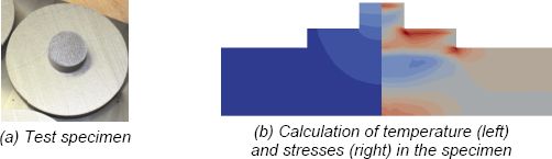
Figure 2.27. Thermomechanical numerical simulation of an additive manufacturing process on a specimen (source: © ArianeGroup). For a color version of this figure, see www.iste.co.uk/sigrist/simulation2.zip
COMMENT ON FIGURE 2.27.– The figure shows a calculation of the temperature and stress fields in a test specimen obtained by the “laser powder bed fusion” process. The simulation, which accounts for the thermal and mechanical phenomena that develop in the part, uses the so-called “element activation” technique. The numerical model is built from a mesh in which the computational elements are gradually integrated into the simulation, thus solving the equations on a domain updated during the computation, in order to represent the material additions. This type of simulation, operated on a model made up of small meshes, mobilizes a computer for nearly 20 h. It is useful to engineers to calibrate process parameters, including heat source application time, heat flow power and material cooling time.
“As part of the development projects for ‘Factory 4.0’ within ArianeGroup, more efficient simulation tools are being deployed in design offices and manufacturing methods. These simulations are based on a mechanical calculation, which is less expensive than a calculation that ‘explicitly’ includes thermal effects. The latter are represented ‘implicitly’ by induced deformations, which are identified by means of test or calibration specimens for a given material and process. This method, known as the ‘inherent deformations’ method, also used in the numerical simulation of welding for large structures, is used as a standard for the development of complex part manufacturing ranges”.
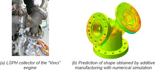
Figure 2.28. Additive manufacturing of a real part: numerical simulation with the “inherent deformations” method (source: © ArianeGroup). For a color version of this figure, see www.iste.co.uk/sigrist/simulation2.zip
COMMENT ON FIGURE 2.28.– Simulation of additive manufacturing processes with the “inherent deformation” method makes a good compromise between accuracy and computation time. Integrating all the physics, it allows us to anticipate the deformations undergone by the part during its manufacture with a reliability considered very satisfactory by the engineers. The calculation presented here gives the final state of an engine component for the Ariane VI rocket. It is carried out using a calculation code used by design engineers, to whom research engineers occasionally provide the technical expertise necessary for the implementation or interpretation of the calculation results.
This type of numerical approach to additive manufacturing is nowadays implemented by many manufacturers, particularly in the aerospace and maritime construction sector (Airbus, Safran, ArianeGroup, Naval Group, etc.). Contributing to the renewal of industrial production methods, additive manufacturing is becoming one of the essential components of tomorrow’s plant, which is progressing in conjunction with numerical simulation.
2.4. Improving performance
2.4.1. Increasing seaworthiness
In 2016, the Modern Express, a cargo ship more than 150 m long, flying the Panamanian flag and carrying nearly 4,000 tons of wood, drifted for several days off the French and Spanish coast. Lying on its side, listing, it was at risk of letting in water, and its fuel polluting the ocean. The ballast tanks, used to improve the stability of the ships, were not operated properly by the cargo ship’s crew: filled on the wrong side of the ship, they increased the ship’s inclination, instead of decreasing it in dangerous sea conditions. Such a situation, attributed to human error, happens only rarely. It is, as far as possible, anticipated at the time of ship design: stability studies, for example, are among the most stringent regulatory requirements in shipbuilding (Figure 2.29).
From the comfort of the passengers on board cruise ships to the integrity of the cargo loaded on a merchant ship, to delicate maneuvers such as landing a helicopter on a frigate: sea-keeping is about the operability and safety of all marine platforms. Many calculation methods contribute to this, explains Jean-Jacques Maisonneuve, an expert in the field at Naval Group/Sirehna:
“The overall behavior of an offshore platform is first studied by means of ‘wave calculations’: from a three-dimensional model of the ship, engineers calculate the amplitude of its movements (three translations and three rotations) when it receives a wave whose frequency and relative direction in relation to the hull are known. Determined for each vessel by means of specific calculation codes, these ‘transfer functions’ are calculated once and for all. They are then used to evaluate more complex sea configurations, combining the amplitudes of motion calculated for the basic directions”.
A statistical calculation is used to evaluate the displacements, accelerations or forces experienced by the ship during its overall movement in response to different swells, according to their amplitude, and for different speeds or impacts of the vessel encountering them (Figure 2.30).
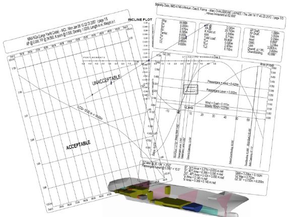
Figure 2.29. Stability study of a ship, carried out with the MAAT-Hydro calculation code
(source: Marc Chausserie-Laprée/www.mchl.fr)
COMMENT ON FIGURE 2.29.– The stability curve shows how a vessel’s “righting torque” evolves as a function of its heel angle. A positive torque arm means that the combined effect of the hydrostatic thrust and weight of the vessel in the opposite direction tends to return it to its original position when it moves away from it: the boat is stable. The area under the stability curve indicates the mechanical energy required to heel the vessel to a given angle. It is used to assess the ship’s righting ability and it yields useful data for engineers conducting stability studies. “When they were defined by the International Maritime Organization (IMO) in the late 1980s, the general opinion was that regulatory stability criteria should be developed in the light of the statistical analysis of the stability parameters of ships involved in accidents and of ships operating safely. Conducted by the IMO in 1966 and 1985, this vast survey made it possible to prescribe the stability criteria that its member countries can apply in their national regulations”, explains Marc Chausserie-Laprée, a naval engineer and expert on these issues. “These criteria were initially developed for cargo, passenger and fishing vessels. They were then extended to other types of ‘ships’: drilling platforms, dredging equipment, submarines, yachts, etc.”. Stability calculations are performed assuming the vessel is stationary and navigates in calm water. A stability curve is calculated with the shape of the hull and the load cases as input data. These consist of the characteristics of the vessel in the light state calculated from the “mass estimate” (mass distribution of bulkheads, decks, materials, equipment, etc.), to which are added various loading conditions according to the type of vessel: passengers, containers, fish, etc. The “consumable” products such as fuel and water are then added: they vary during navigation and therefore require the calculation of different loading cases. The “free surface” effect, intrinsically variable, should also be taken into account: in partially filled tanks, the movement of fluids changes the position of the ship’s center of gravity and may thus reduce its stability. The damage stability calculations of one or more compartments are much more complex. “The so-called ‘probabilistic’ stability requires, for example, calculating several thousand stability curves by combining several hundred damage cases for different loading conditions. The software calculates the probability that certain compartment assemblies will be flooded simultaneously and the probability that the vessel will ‘survive’ this damage. Several hours of calculation are then required to be compared with the stability analysis for an intact ship, which is obtained almost instantaneously”.
The data thus produced are compared with operability criteria, making it possible to demonstrate the ship’s operational safety under the most probable sea conditions.
“Wave response calculation methods give indications of the ship’s behavior at sea… but cannot account for certain situations encountered more rarely in difficult sea conditions. Waves breaking on a ship’s deck, the impacts of the bow on waves, etc. Engineers study these configurations using numerical simulations based on the ‘complete’ equations of fluid mechanics”.
In some cases, the models aim to represent both the ship’s movements and the hydrodynamics of the flow. Representing this “fluid/structure interaction” (Box 2.2) is necessary, for example, to study a ship stabilization system using controllable fins (Figures 2.31 and 2.32). Allowing the system and its operation to be accurately represented, simulations are carried out in an effort to improve current solutions.

Figure 2.30. Analysis of sea-keeping (source: Sirehna/Naval Group). For a color version of this figure, see www.iste.co.uk/sigrist/simulation2.zip
COMMENT ON FIGURE 2.30.– The sea-keeping analysis is based on data describing the hydrodynamic loading and on a numerical model of the vessel. The wave spectrum (a) represents the amplitude of waves according to their frequency in all directions; the calculation makes it possible to evaluate the amplitude of the ship’s movements at different incidences (b) according to the wave period.
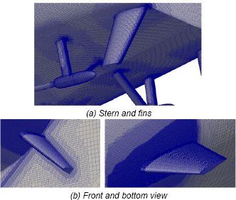
Figure 2.31. Numerical model of a ship with stabilizer fins [YVI 14]. For a color version of this figure, see www.iste.co.uk/sigrist/simulation2.zip

Figure 2.32. Simulation of wave resistance [YV1 14]. For a color version of this figure, see www.iste.co.uk/sigrist/simulation2.zip
COMMENT ON FIGURE 2.32.– The figure shows the calculation of the vessel’s rolling condition with passive (left) and active (right) stabilizing fins for two moments of oscillation. The simulation is used to represent the increase in the free surface level and the value of the pressure coefficient in both cases. It highlights the contribution of the active stabilization device.
2.4.2. Limiting noise pollution
Published in 1837, Les voix intérieures is a collection of poems by Victor Hugo (1802-1885), in which the writer seems to celebrate these times of introspection, which flourish ideally in periods of calm. In these moments of meditation, sounds, sometimes giving all their relief to silence, are not as harmonious or soft to our ears as those from a distant sea, which one hears without seeing:
What’s this rough sound?
Hark, hark at the waves,
this voice profound
that endlessly grieves
nor ceases to scold
and yet shall be drowned
by one louder, at last:
The sea-trumpets wield
their trumpet-blast.
(Une nuit qu’on entendait la mer sans la voir, [HUG 69], translation by Timothy Adès4.
The transport industry in general, and the air and maritime transport industries in particular, is one of the most involved in the search for technical solutions to reduce noise pollution. The control of acoustic signatures of maritime platforms is therefore a major challenge for manufacturers in the naval sector5:
- – for manufacturers of passenger ships, being able to justify a comfort brand is a factor that sets them apart from the competition. It thus meets an increased demand from ship owners: the noise and vibration criteria, defined in terms of permissible noise levels in cabins, for example, are becoming more and more stringent in the ship’s specifications;
- – for military naval shipbuilders, controlling the ship’s acoustic signature is an essential element in order to guarantee its stealth in many operational conditions. The constraints of submarine stealthiness, for example, popularized by the fiction The Hunt for Red October [CLA 84, TIE 90], are among the strongest in their design [BOV 16, REN 15]. Numerical simulation is a tool that is increasingly used in various stages to demonstrate and justify the expected vibration performance (Figure 2.33).
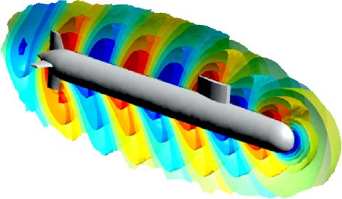
Figure 2.33. Numerical simulation of ship vibrations: example of acoustic radiation from a submarine [ANT 12]. For a color version of this figure, see www.iste.co.uk/sigrist/simulation2.zip
COMMENT ON FIGURE 2.33.– The numerical models used by shipbuilding engineers strive to reflect the dynamic behavior of the ship to scale. They include many structural details, such as decks, bulkheads, superstructures, engines, and so on, and a modeling of different materials performing different functions (structural resistance, soundproofing, fireproofing – and, in some cases, even decoration!). Depending on practice, models may include finite elements of different types (shells, beams, volume or point elements, connecting elements, etc.) in order to accurately represent the ship. The number of equations to be solved in this model thus becomes significant, containing several hundred thousand, even a few million, degrees of freedom, and the calculations require appropriate computer resources.
The propulsive chain, consisting of the engines, transmission and power conversion components (shaft line, speed reducer, propeller, etc.), is the main source of noise on a ship [BOV 16]. This spreads through the inner structures and the hull into the ocean and designers seek to limit it, for example by using damping devices (Figure 2.34).

Figure 2.34. Numerical model of a suspension mount [PET 12]. For a color version of this figure, see www.iste.co.uk/sigrist/simulation2.zip
COMMENT ON FIGURE 2.34.– Made of elastomeric materials, suspension mounts are used in many land, sea and air vehicles. They are designed to isolate a machine or equipment, thereby helping to limit the noise emitted by the former and reduce the vulnerability of the latter to shock and vibration. Numerical modeling helps to optimize, for example, their damping performance. Simulations require a detailed representation of the mechanical behavior of elastomeric materials in a wide range of operating ranges.
Turbulent flows are also a source of vibratory excitation of many structures [PAI 04, PAI 11]. These phenomena occur in various situations, for example:
- – aerodynamic or hydrodynamic lifting profiles (aircraft wings, ship rudders or propellers, etc.) or bluffed bodies (solar panels, tiles, cables, towers, chimneys, etc.);
- – energy generation and recovery devices (tube bundles, wind turbines, hydroturbines, fluid networks, etc.).
These vibrations are associated with undesirable effects:
- – premature wear and tear, which can jeopardize the safety of installations;
- – significant noise emissions, a source of noise pollution impacting ecosystems, or discomfort for passengers on means of transport.
Turbulent flows (Figure 2.35) also generate vibrations among the structural elements of ships (hull, deck, etc.): these are among the many possible causes of submarines’ acoustic indiscretions.

Figure 2.35. Development of a turbulent boundary layer on a wall
COMMENT ON FIGURE 2.35.– When the fluid flow on a wall becomes turbulent, the wall pressure fluctuates significantly. The various turbulent structures developing in the flow carry an energy, more or less significant according to their size, sufficient to cause vibrations. The physics of the turbulent boundary layer, and its different regimes, is well characterized by researchers in fluid mechanics who base their knowledge on numerous experimental studies [SCH 79].
Engineers have a lot of empirical data on turbulent excitation. These are represented by turbulence spectra representing the intensity of the turbulent pressure field over a given frequency range (see Figure 2.36). The figure highlights the variability of the experimental data: this is one of the difficulties faced by engineers.

Figure 2.36. Empirical spectra of turbulent excitation [BER 14]. For a color version of this figure, see www.iste.co.uk/sigris1/simulation2.zip
COMMENT ON FIGURE 2.36.– The figure shows several models of turbulent excitation spectra, obtained by different fluid mechanics researchers for “simple” flow configurations [CHA 80, EFI82, GOO 04, SMO 91, SMO 06]. The spectrum gives the evolution of the pressure according to its frequency of fluctuation. The quantities are represented in the conventional form, known to experts in the field. The data are obtained in “ideal” configurations, which are often far from real applications. Despite their limitations in validity, in some cases they are the only information available to engineers to analyze turbulence-induced vibrations.
Which model is the most suitable for calculations? What are the variations in the simulation results? To what extent are they attributable to the input data? Numerical simulation helps to answer such questions and reduce the degree of empiricism that remains in some flow-induced vibration calculations, as explained by Cédric Leblond, an expert in the field at Naval Group:
“We use numerical simulation of turbulent flows with RANS methods to feed a theoretical model which calculates turbulent excitation spectra in more general configurations than those delimiting the current validity of empirical spectra. Calculations are used to extract data characterizing the physics of the turbulent boundary layer. The models we develop use this information to calculate the fields contained in the equations describing the evolution of the pressure field”.
With this so-called “hybrid approach” [SLA 18], engineers take advantage of the accuracy of numerical calculations and combine it with the ease of use of turbulent excitation spectra. Validated on simple configurations (Figure 2.37), the method allows them to calculate excitation spectra for configurations representative of actual ship navigation conditions.
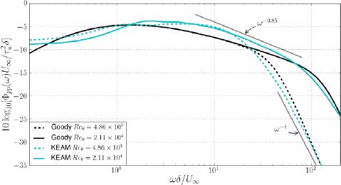
Figure 2.37. Numerically calculated and empirically determined turbulent excitation spectrum [SLA 17]. For a color version of this figure, see www.iste.co.uk/sigrist/simulation2.zip
COMMENT ON FIGURE 2.37.– The figure shows the turbulent excitation spectra corresponding to two simple water flow configurations – on a flat wall, at two different speeds. The quantities are represented in the conventional form, known to experts in the field. Spectra calculated with a numerical method are represented as green lines, and spectra determined with an empirical model as black lines. The figure shows that the two types of spectra are very close, which validates the numerical calculation method. The latter can be used by engineers to calculate excitation spectra for real configurations, while empirical spectra may only be valid in particular situations.
More accurate turbulent flow calculations allow for a direct characterization of turbulent excitation. Simulations are very expensive when they represent increasingly fine-grained turbulence scales, so researchers are constantly improving numerical methods.
One of the challenges in aeronautical and ship-building is to calculate flows around large objects, with a resolution fine enough to capture the details of vortex dynamics. Solving the Navier–Stokes equation requires very fine mesh sizes, especially near a wall. In some flow configurations, the size of the models to be implemented in a calculation becomes an obstacle to the implementation of simulations for industrial applications.
Simulations based on other models than the one contained in the Navier–Stokes equations make it possible to reduce the cost of calculation while maintaining such fine mesh sizes. The Lattice Boltzmann Method (LBM*) is one of them. Widely used for compressible flow simulations such as those encountered in aeronautics and the automotive industry, it has developed in these sectors over the past decade. Aloïs Sengissen, expert engineer of this method at Airbus, comments:
“Flow simulations based on an average description of Navier-Stokes equations (the RANS models), allows for calculation at computational costs that are compatible with project deadlines. They give good results when we try to evaluate the aerodynamic characteristics of aircraft, for instance. Providing average quantities (pressure, speed), they are unsuitable for aero-acoustic problems, studied, for example, for the prediction of noises which by nature are unsteady phenomena. Finer methods, such as simulating the main turbulence scales from the Navier-Stokes equation (LES modeling), are too time-consuming to model and calculate. The LBM method, the development of which has benefited from innovations in HPC calculation, offers us the possibility of finely simulating flows, at modeling and calculation times acceptable for many industrial applications”.
This method is based on the Boltzmann6 equation, which describes flows at a scale different from that underlying the Navier–Stokes model. By taking a step back, it is possible to categorize flow modeling according to three scales typically used by fluid physicists:
- – representing the interactions between fluid particles, such as gases, the “microscopic” description requires solving a large number of degrees of freedom. It is a question of describing, according to the principle of action/reaction explained by Newton’s third law, the force exerted by each particle on the others. This approach is out of reach for dense flows;
- – at the opposite end, translating the principles of conservation of mass, momentum and energy, the Navier–Stokes equations describe flow on a “macroscopic” scale;
- – Boltzmann’s equation models the flow at the “mesoscopic” scale, intermediate between the two previous ones. Taking as unknown mathematical functions that account for the statistical distribution of particles in a flow, Boltzmann’s model describes their kinetics using a transport equation, accounting for collisions and particle propagation. The flow quantities, useful to engineers (such as pressure and energy), are deduced from the distribution functions thus calculated.
Solving the Boltzmann equation does not necessarily require a structured mesh coinciding with a wall, as required by the finite volume method (Figure 2.38). This contributes to the effectiveness of the LBM method, comments Jean-François Boussuge, a researcher at CERFACS*:
“Algorithms developed in the LBM report on the propagation of particles and the collisions they undergo. These are calculated for points constituting a network, which can be refined more immediately than the calculation mesh deployed for solving the Navier-Stokes equations. The network can thus be precisely adapted to complex geometries, taking into account the structural details of aircraft, automobiles, etc., which must be represented for acoustic studies. It is these singularities that are responsible for the pressure fluctuations causing vibrations and noise generated by the flow”.
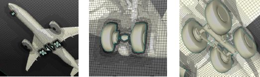
Figure 2.38. The calculation grid used in the Lattice Boltzmann Method can be adapted to complex geometries
(source: © Airbus)
In response to the need of designers to have simulation of unsteady phenomena, particularly necessary to estimate flow noise, the LBM is nowadays used by many engineers in the aeronautics and automotive industry (Figure 2.39). Aloïs Sengissen testifies:
“From acoustics to aerodynamics to thermics, we are now simulating many fluid dynamics problems using the Lattice Boltzmann Method. The simulation is used to address some unsteady flight configurations, such as the near stall flight regime, where a loss of lift is feared. LBM is particularly effective using ‘massively parallel’ algorithms and allows calculations to be carried out in these situations, which would not be accessible to us with any other numerical methods”.
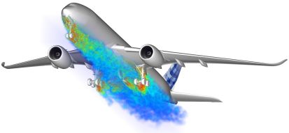
Figure 2.39. Flow simulation on an aircraft using the Lattice-Boltzmann method (source: ©Airbus). For a color version of this figure, see www.iste.co.uk/sigrist/simulation2.zip
COMMENT ON FIGURE 2.39.– The figure shows a numerical simulation of a weakly compressible turbulent flow around an Airbus aircraft. The objective of the calculation is to capture as accurately as possible the wake dynamics generated downstream of the nose landing gear. Impacting rear axle doors, the intensity of the vibrations generated by vortices particularly affects gear noise or mechanical wear. The calculations thus help to predict their life expectancy. Such a simulation uses a numerical model of significant size. Several hundred and even thousands of processors operate in parallel on a supercomputer in order to realize it [SEN 15].
2.4.3. Protecting from corrosion
Corrosion is an alteration of a material by chemical reaction and is feared by plant designers and operators in many economic sectors, particularly marine platforms. By taking into account all means of combating corrosion, replacing corroded parts or structures, as well as the direct and indirect consequences of the accidents it causes, corrosion induces costs that are estimated at nearly 2% of the world’s gross product and consume, for example, nearly 300 million tons of steel each year [NAC 02].
Corrosion affects, to varying degrees, all kinds of materials (metallic, ceramic, composite, elastomeric, etc.) in varying environments. The corrosion of metals results, in the vast majority of cases, from an electrochemical reaction involving a manufactured part and its environment as reagents.
A “multi-physical” problem par excellence, corrosion can be approached by numerical simulation, explains Bertil Nistad, modeling expert at COMSOL:
“The finest simulations are based on a set of equations that capture in as much detail as possible the electrical, chemical and mechanical phenomena involved in corrosion. The models describe the environment and electrical state of the part studied, in terms of concentration of charged species, oxygen levels, surface treatments and protections, or presence of marine deposits, etc. and are generally supplemented by experimental data. The finite element method is one of the most widely used in simulations: it solves model equations – the most elaborate of which are based on nearly ten non-linear and coupled equations”.
Calculations allow us to, for example, understand the physics of the phenomena involved [KOL 14, WAT 91], as illustrated in Figure 2.40. They can help to evaluate the effectiveness of a protection system, such as cathodic protection. The latter reduces the corrosion rate of a metallic material in the presence of an aqueous medium. By circulating an electrical current between an auxiliary electrode and the material to be protected, the latter is placed at such an electrical potential that the corrosion rate becomes acceptable over the entire metal surface in contact with the aqueous medium. The simulation optimizes the placement of the electrodes to ensure optimal protection (Figure 2.41).
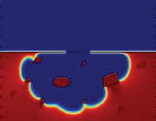
Figure 2.40. Simulation helps to understand the evolution of corrosion. For a color version of this figure, see www.iste.co.uk/sigrist/simulation2.zip
COMMENT ON FIGURE 2.40.– The figure is an example of a simulation of the development of point corrosion: the numerical method is used to represent and evaluate the propagation of the corroded material front [QAS 18].

Figure 2.41. Modeling of a corrosion protection system for a ship’s hull (source: image produced with the COMSOL Multiphysics® code and provided by COMSOL/ www.comsol.fr). For a color version of this figure, see www.iste.co.uk/sigrist/simulation2.zip
COMMENT ON FIGURE 2.41.– The figure shows the electrical current map calculated around a ship’s hull equipped with a protective electrode. By identifying areas likely to present favorable conditions for the development of corrosion, the simulation helps to optimize the design of the protection device. This type of simulation also makes it possible to dimension it by limiting its electrical signature, an important issue to ensure the discretion of certain military vessels, such as submarines [HAN 12].
Beyond this example of application to the naval field, corrosion simulation is of interest to many industrial sectors, such as offshore construction, nuclear energy, rail transport and steel construction as a whole.
2.4.4. Reducing energy consumption
The shape of car bodies has been constantly refined to achieve remarkable aerodynamic performance today, helping to reduce fuel consumption. Shipbuilders also proceed in the same way, seeking the most efficient forms of hulls to satisfy sometimes demanding sailing criteria – in particular in terms of seaworthiness, an environment that is in some respects more restrictive than land.
Pol Muller, hydrodynamics expert at Sirehna/Naval Group, explains how numerical simulation fits into a loop for optimizing hull shapes:
“We have developed a digital strategy that helps to design ‘optimal’ hull shapes for different design constraints and performance objectives. The first are, for example, the stability of the ship, its transport capacity, when one of the second is, for example, the reduction of the resistance to forward motion, which directly influences energy consumption”.
This optimization approach is known as “multicriteria” because it aims to take into account all design parameters in the analysis that takes place in several stages. Carried out for the first time on a small trawler, it is generic and now applies operationally to all types of vessels.
“Starting from a hull shape established according to state-of-the-art techniques, we first explore different possible shapes, varying the dimensions using a ‘parametric modeler’. Carrying out the operation automatically, this tool makes it possible to create a set of different shapes according to ‘realistic’ architectural choices: length and width of the ship, angle of entry of water from the bow, etc. In a second step, we determine by means of more or less complex calculations the different performance criteria of these virtual vessels. Stability is assessed by means of graphs, when the resistance to forward motion requires fluid dynamics simulations, for example”.
The entire process is automated and preliminary tests guarantee the robustness of the developed calculation chain. It can be used as a decision support tool, with engineers analyzing certain calculations in order to understand the influence of a design parameter on the ship’s performance, or as an optimization tool (Figure 2.42), with the algorithm selecting parameters that can satisfy the constraints of the calculation (e.g. stability requirements) and work toward the objectives set (e.g. minimizing resistance to forward motion).
After some modifications by naval architects, the shape determined by the algorithm is then manufactured. A sea testing campaign with both types of hulls validates the simulation models, on the one hand, and the performance predictions given by the calculation, on the other hand (Figure 2.43).

Figure 2.42. Optimization of hull shape (source: ©Sirehna/Naval Group). Fora color version of this figure, see www.iste.co.uk/sigrist/simulation2.zip
COMMENT ON FIGURE 2.42.– The figure represents the initial shape of a trawler’s hull, which is then modified by the optimization algorithm to achieve lower fuel consumption, while meeting the vessel’s operational requirements. In the process, a fluid dynamics calculation is performed to evaluate the vessel’s resistance to forward motion.
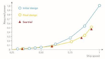
Figure 2.43. Comparison of hull performance for different ship speeds (source: Sirehna/Naval Group). For a color version of this figure, see www.iste.co.uk/sigrist/simulation2.zip
COMMENT ON FIGURE 2.43.– The figure shows the evolution of the ship’s power as a function of its navigation speed (the data are presented in a dimensionless form). The comparison of sea trial data with the calculation results highlights the reliability of the simulation process. The comparison of the two hull shapes, initial and final design, shows the gains obtained in terms of energy consumption: it is reduced by nearly 40% at the highest speeds.
Numerical simulation changes the practices of engineers in the industry and also gives them the opportunity to develop them. To this end, practitioners must also rethink their relationship to the tool they use – this is reflected in Pol Muller, who is left to conclude this chapter:
“Because it is not constrained by any ‘preconceived notion’ or ‘empirical reflex’, the algorithm can sometimes be more ‘creative’ than a naval engineer! Exploring forms that intuition can initially reject, the algorithm can thus allow architects to become aware that bold choices, offering unexpected performances, are possible… and above all feasible!”
- 1 Animals contributed just like humans to the exploration of the skies: in the 20th Century, the Russian dog Laika was the passenger of the spaceship Sputnik 2; her stay in space in November 1957 preceded, by a few years, that of Yuri Gagarin (1934–1968) who became, in April 1961, the first human in space.
- 2 However, the A380, which has been in service with many international airlines since its entry into service, has not been able to consolidate its place in the air in the long term, perhaps a victim of its size. In 2019, due to the lack of a sufficiently large order book, Airbus announced that it would cease production of this non-standard aircraft [JOL 19].
- 3 The baptism of the “Saint Exupéry” in 2018 was accompanied in France by particular questions on the environmental impact of maritime transport, in a context where the sector remained one of the last outside the Paris Agreement of 2015. It should be noted that in 2018, the 174 Member States of the IMO (International Maritime Organisation, dependent of the United Nations) agreed on a quantified objective to reduce greenhouse gas emissions, aiming to reduce them by half by 2050 [HAR 18].
- 4 http://www.timothyades.co.uk/victor-hugo-une-nuit-qu-on-entendait-la-mer-sans-la-voir.
- 5 It should be noted that the study of noise and vibration is not only aimed at the acoustic comfort of human beings: the impact of noise pollution on underwater fauna (cetaceans, cephalopods, etc.) is scientifically highlighted and is receiving increasing attention.
- 6 Established by the Austrian physicist Ludwig Eduard Boltzmann (1844–1906), who helped to develop a mathematical formalism adapted to the statistical description of fluids.