Chapter 9

The Use of Hidden Markov Models for Image Recognition: Learning with Artificial Ants, Genetic Algorithms and Particle Swarm Optimization

9.1. Introduction

Hidden Markov models (HMMs) are statistical tools which are used to model stochastic processes. These models are used in several different scientific domains [CAP 01] such as speech recognition, biology and bioinformatics, image recognition, document organization and indexing as well as the prediction of time series, etc. In order to use these HMMs efficiently, it is necessary to train them to be able to carry out a specific task. In this chapter we will show how this problem of training an HMM to carry out a specific task can be resolved with the help of several different population-based metaheuristics.

In order to explain what HMMs are, we will introduce the principles, notations and main algorithms which make up the theory of hidden Markov models. We will then continue this chapter by introducing the different metaheuristics which have been considered to train HMMs: an evolutionary method, an artificial ant algorithm and a particle swarm technique. We will finish the chapter by analyzing and evaluating six different adaptations of the above metaheuristics that enable us to learn HMMs from data which comes from the images.

9.2. Hidden Markov models (HMMs)

HMMs have existed for a long time. They were defined in 1913 when A. A. Markov first designed what we know as Markov chains [MAR 13]. The first efficient HMM algorithms and the key principles of HMMs only appeared during the 1960s and 1970s [BAU 67, VIT 67, BAU 72, FOR 73]. Since then, several variants of the original HMMs have been created and a number of HMM applications have been a success. In order to give precise definitions, we need to define what we consider to be a discrete hidden Markov model throughout this chapter.

9.2.1. Definition

A discrete hidden Markov model corresponds to the modeling of two stochastic processes. The first process corresponds to a hidden process which is modeled by a discrete Markov chain and the second corresponds to an observed process which depends on the states of the hidden process.

DEFINITION 9.1. Let = {s₁, . . . , s_N} be the set of N hidden states of the system and let S = (S₁, . . . , S_T) be a tuple of T random variables defined on . Let = {υ₁, . . . , υ_M} be the set of the M symbols which can be emitted by the system and let V = (V₁, . . . , V_T) be a tuple of T random variables defined on . It is therefore possible to define a first order discrete hidden Markov model by using the following probabilities:

• the initialization probability of hidden states: P (S₁ = s_i),
• the transition probability between hidden states: P (S_t = s_j | S_t−1 = s_i),
• the emission probability of the symbols for each hidden state: P (V_t = υ_j | S_t = s_i).

If the hidden Markov model is stationary then the transition probability between hidden states and the emission probability of the symbols for each hidden state are independent of the time t > 1. For every value of t > 1, we can define A = (a_i,j)_1≤i,j≤N with a_i,j = P (S_t = s_j | S_t−1 = s_i), B = (b_i(j))_{1≤i≤N, 1≤j≤M} with b_i(j) = P (V_t = υ_j | S_t = s_i) and Π = (π₁, . . . , π_N)′ with π_i = P (S₁ = s_i). A first order stationary hidden Markov model denoted by is therefore defined by the triplet (A, B, Π). Throughout this chapter we will continue to use the notation and we will use the term hidden Markov models (HMM) for the first order stationary HMMs. Let Q = (q₁, . . . , q_T) ^T be a sequence of hidden states and let O = (o₁, . . . , o_T) ^T be a sequence of observed symbols. The probability of producing a sequence of hidden states Q and of producing a sequence of observations O according to the HMM is written as follows:¹

P(V = O, S = Q | A, B, Π) = P(V = O, S = Q | )

The conditional probabilities lead to:

From an HMM , a sequence of hidden states Q and a sequence of observations O, it is possible to calculate the balance between the model and the sequences Q and O. In order to be able to do this, we only need to calculate the probability P (V = O, S = Q | ). This probability corresponds to the probability of a sequence of observations O being produced by the model after a sequence of hidden states Q has been produced.

Whenever the sequence of states is unknown, it is possible to evaluate the likelihood of a sequence of observations O according to the model . The likelihood of a sequence of observations corresponds to the probability P (V = O|) that the sequence of observations has been produced by the model when considering all the possible sequences of hidden states. The following formula is therefore validated:

Whenever HMMs are used, three fundamental issues need to be resolved (for the model ):

– evaluating the likelihood of P (V = O|) for a sequence of observations O according to the model . This probability is calculated using the forward or backward algorithm with a complexity level of O(N²T) [RAB 89];

– determining the sequence of hidden states Q^∗ which has most likely been monitored with the aim of producing the sequence of observations O: the sequence of hidden states Q^∗, which is defined by the equation below, is determined by Viterbi’s algorithm with a complexity level of O(N²T) [VIT 67];

– training/learning one or several HMMs from one or several sequences of observations whenever the exact number of hidden states of the HMMs is known. Training the HMMs can be seen as a maximization problem of a criterion with the fact that the matrices A, B and Π are stochastics. A number of different criteria exist which can be used.

9.2.2. The criteria used in programming hidden Markov models

In the following, an optimal model for a given criterion is noted as ^∗ and is used to represent the set of HMMs that exist for a given number of hidden states N and a given number of symbols M. O is the sequence of observations that is to be learned. During our research, we found that five different types of training criteria exist:

– the first type of criteria is the maximization of the likelihood. The aim of these criteria is to find the HMM ^∗ which validates the equation:

However, no specific or general methods exist for this type of criteria. Nevertheless, the Baum-Welch (BW) algorithm [BAU 67] and the gradient descent algorithm [KAP 98, GAN 99] make it possible, from an initial HMM, to improve it according to the criterion. These algorithms converge and lead to the creation of local optima of the criterion;

– the second type of criteria is the maximization of a posteriori probabilities. The aim of these criteria is to determine the HMM ^∗ which validates the equation:

This type of criteria, which is associated with the Bayesian decision theory [BER 98], can be divided into a number of smaller criteria depending on the aspects of the decision theory that are being investigated. The simplest forms of this criterion lead to maximum likelihood problems. However, the more complex forms of this criterion do not allow for this possibility. For the more complex forms it is possible to use a gradient descent algorithm in order to investigate such issues. In all cases, the resulting models are local optima of the criteria;

– The third type of criteria is the maximization of mutual information. The aim of these criteria is to simultaneously optimize several HMMs with the aim of maximizing the discrimination power of each HMM. This type of criteria has been used on several occasions in several different forms [RAB 89, SCH 97, GIU 02, VER 04]. One of the solutions that is available and which can be used to maximize these criteria is the use of a gradient descent algorithm. Once again the results which are obtained are local optima of the criteria.

– The fourth type of criteria is the minimization of classification errors of the observation sequences. Several forms of these criteria have been used [LJO 90, GAN 99, SAU 00]. In the three previous types of criteria, the criteria are non-derivable and they are also not continuous. In order to maximize the three previous types of criteria, the criteria are usually approximated with derivable functions. Gradient descent techniques are then used.

– The fifth and final type of criteria is segmental k-means criteria. The aim of these criteria is to determine the HMM ^∗ which validates the equation:

is the sequence of hidden states which is obtained after the Viterbi algorithm [VIT 67] has been applied to the HMM . As far as segmental k-means is concerned, the aim is to find the HMM which possesses the sequence of hidden states which has been monitored the most. One of the main characteristics of this criterion is that it is neither derivable nor continuous. One solution consists of approximating the criterion by applying a derivable or at least a continuous function to it; however developing such a solution for the moment is a difficult task. It is possible, however, to use the segmental k-means algorithm [JUA 90] to partially maximize this criterion. The way in which this algorithm functions is similar to the way in which the Baum-Welch algorithm functions for maximum likelihood. The segmental k-means algorithm iteratively improves an original HMM and also makes it possible to find a local optimum of the criterion.

We have noticed that numerous criteria can be considered when it comes to training HMM. The criteria which have been described in this section are not the only criteria that can be used but they are the ones that are used the most often. For the majority of these criteria there is at least one corresponding algorithm that exists and which can be used in order to maximize the criteria. These algorithms, which are applied to an initial model, lead to the creation of a new model which in turn improves the value of the said criterion. This approach makes it possible to calculate a local optimum of the criterion in question, but not a global optimum. In certain cases, a local optimum is sufficient, but this is not always the case. It is therefore necessary to be able to find optimal models, or at least find models which resemble, from the point of view of the criterion t an optimal solution of a criterion. One possibility consists of using metaheuristics [DRE 03] with the aim of investigating and exploring HMMs.

9.3. Using metaheuristics to learn HMMs

The aim of this section is to describe the principal metaheuristics that are used to train HMMs. Before we introduce the different metaheuristics, we believe that it is a good idea to introduce the three different types of solution spaces which have been used up until now.

9.3.1. The different types of solution spaces used for the training of HMMs

It is possible to consider three types of solution spaces which can be used to train HMMs [AUP 05a]: Λ, ^T and Ω. In order to describe the different solution spaces, we consider HMMs possessing N hidden states and M symbols, and sequences of observations O with a length of T.

9.3.1.1. Λ solution space

The Λ solution space is the solution space which is the most commonly used for training HMMs. This type of solution space corresponds to the set of stochastic matrix triplets (A, B, Π) which define a HMM. Λ is therefore isomorphic to the Cartesian product _N × (_N)^N × (_M)^N where _K is the set of all stochastic vectors with K dimensions. _K possesses the fundamental property of being convex which implies that Λ is also convex.

9.3.1.2. ^T solution space

The ^T solution space corresponds to the set of hidden state sequences where each sequence is of length T . The fundamental properties of this type of solution space are that it is discrete, finite and is composed of N^T elements. An HMM is defined by its triplet of stochastic matrices, then any given solution of ^T cannot be directly used as an HMM. Instead, a labeled learning algorithm is used in order to transform the hidden state sequence into an HMM. The labeled learning algorithm estimates probabilities by computing frequencies. γ(Q) is the model which is created after the labeled learning algorithm has been applied to the sequence of observations O and to the sequence of states Q ^T. The set γ(^T) = {γ(Q) | Q ^T} is a finite subset of Λ. The function γ is neither injective, nor surjective and as a consequence it is not possible to use an algorithm such as the Baum-Welch algorithm with this type of solution.

9.3.1.3. Ω solution space

The Ω solution space was initially defined with the aim of providing a vector space structure for the training of HMMs [AUP 05a]. With this in mind, we consider the set _K of stochastic vectors with K dimensions. We define as a subset of stochastic vectors with dimension K. None of the components of this subset have a value of zero, in other words . Therefore is a regularization function which is defined on ^K by the following equation:

where r_K(x)_i is the ith component of the vector r_K(x).

We define and three symmetric operators and so that for all values (x, y) (Ω_K)² and c :

Then (Ω_K, _K, _K) is a vector space. Let and two operators. These operators can transform the elements of into elements of Ω_K, and vice-versa with the help of the equations below (for all values of and for all values y Ω_K):

We define Ω as Ω = Ω_N × (Ω_N)^N × (Ω_M)^N and Λ^∗ as . By generalizing the operators and _K to the Cartesian products Ω and Λ^∗, and by removing the K index, we can prove that (Ω, , ) is a vector space, and that (Λ^∗) = Ω and (Ω) = Λ^∗. It is also important to note that Λ^∗ Λ.

9.3.2. The metaheuristics used for the training of the HMMs

The six main types of metaheuristics that have been adapted to the HMM training problem are: simulated annealing [KIR 83], Tabu search [GLO 86, GLO 89a, GLO 89b, HER 92, GLO 97], genetic algorithms [HOL 75, GOL 89], population-based incremental learning [BUL 94, BUL 95], ant-colony-based optimization algorithms such as the API algorithm (API) [MON 00a, MON 00b] and particle swarm optimization (PSO) [KEN 95, CLE 05].

As mentioned earlier in this chapter numerous metaheuristics have been used to train HMMs. When some of the metaheuristics were applied to the HMMs it led to the creation of several adaptations of these metaheuristics (see Table 9.1). These adaptations were not all created with the aim of maximizing the same criterion² and they do not explore nor investigate the same solution space (see Table 9.1).

Table 9.1. Adaptations of the metaheuristics in relation to the three different solution spaces used for training HMM

The use of these metaheuristics raises the issue of size: we do not know which metaheuristic is the most efficient. The metaheuristics have not been compared and no normalized data set has been created which would make it possible to compare the results of performance studies. Even if the data sets were normalized we would still have to deal with the issue of understanding exactly how the algorithms are parameterized. The parameters of the algorithms often correspond to a default choice (or to an empirical choice) rather than corresponding to the best parameters that could make up the algorithm, or at least to the parameters which guarantee a high quality solution. In the next section we will go into more detail about the six adaptations of the generic metaheuristics as well as setting them and finally comparing them with the aim of overcoming some of the problems mentioned in this section. In order to make this possible, we will take the criterion of maximum likelihood as well as the data which comes from the images into consideration.

9.4. Description, parameter setting and evaluation of the six approaches that are used to train HMMs

The algorithms which have been used in this study all consider the maximum likelihood criterion. The six different approaches are the result of the adaptation to the problem of the genetic algorithms, of the API algorithm and of the particle swarm optimization algorithm.

9.4.1. Genetic algorithms

The genetic algorithm [HOL 75, GOL 89] which we have considered in this study is the one that has also been described in [AUP 05a] and can also be seen in Figure 9.1. This algorithm is the result of adding an additional mutation and/or optimization phase of the parents to the GHOSP algorithm which is described in [SLI 99]. For the purpose of our study we have taken two different adaptations of the genetic algorithm into consideration.

The first adaptation of the genetic algorithm uses solutions in Λ. We have called this adaptation of the genetic algorithm AG-A. The chromosome which corresponds to the = (A, B, Π) HMM is the matrix (Π A B) which is obtained by the concatenation of the three stochastic matrices that describe the HMM. The selection operator is an elitist selection operator. The crossover operator is a classical one point (1X) crossover. It randomly chooses a horizontal breaking point within the model (see Figure 9.2). The mutation operator is applied to each coefficient with a probability of p_mut. Whenever the mutation operator is applied to a coefficient h, the mutation operator replaces the coefficient h with the value (1 − θ)h and also adds the quantity θh to another coefficient. This other coefficient is chosen at random and can be found on the same line in the same stochastic matrix. For each mutation the coefficient θ is a number which is uniformly chosen from the interval [0; 1]. The optimization operator then takes _BW iterations from the Baum-Welch algorithm and applies them to the individual (person or child) that needs to be optimized.

Figure 9.1. The principle of the genetic algorithm used in programming the HMMs

Figure 9.2. The principle of the crossover operator (1X) which can be found in the AG-A adaptation of the genetic algorithm

The second adaptation of the genetic algorithm uses the ^T solution space in order to find an HMM. We have called this adaptation of the genetic algorithm AG-B. The individuals are represented by a sequence of hidden states which label the sequence of observations that need to be learned. The corresponding HMM is found thanks to the use of a labeled learning algorithm (for the statistic estimation of the probabilities). The selection operator which is used is once again the elitist selection operator. The crossover operator corresponds to the classical 1X operator of genetic algorithms that use binary representation. The mutation operator modifies each element from the sequence of states with a probability of p_mut. The modification of an element from the sequence involves replacing a state in the solution. The process of optimizing the parents and the children is not carried out because of the non-bijectivity of the labeled learning operator.

The parameters of the two algorithms are as follows: (the size of the population), p_mut (the probability of mutation), MutateParents (do we apply the mutation operator to the parent population?), OptimizeParents (do we apply the optimization operator to the parent population?), and _BW (the number of iterations which is taken from the Baum-Welch algorithm).

9.4.2. The API algorithm

The API algorithm [MON 00a, MON 00b] is an optimization metaheuristic which was inspired by the way in which a population of primitive ants (Pachycondyla apicalis) feed. Whenever the ants’ prey is discovered, this species of ant has the ability to memorize the site at which the prey has been found (the hunting site). The next time the ants leave the nest, they go back to the last site they visited as this is the last one they remember. If, after a number of several different attempts (named as local patience), the ants are unable to find any new prey on the site they give up on the site and do not use it in the future. From time to time the nest is moved to a hunting site. The result of adapting these principles to the global optimization problem has been called the API algorithm (see Algorithm 9.1).

The experiments described in [AUP 05a] show that factors such as the size of the ant colony and the memory capacity of the ants are anti-correlated. As a result of this, we assume that the size of the ant’s memory capacity is one.

In this chapter we deal with three adaptations of the API algorithm. In order to specify the three different adaptations of the algorithm a definition of the initialization operator which refers to the initial position of the nest has been given and we also define the exploration operator.

The first adaptation [MON 00a] of the API algorithm is known as API-A, and the aim of this adaptation of the algorithm is to explore the Λ solution space. The choice of the initial position of the nest is obtained by randomly choosing an HMM within the set Λ. The exploration operator from an existing solution depends on one particular parameter: the amplitude. If we take as the amplitude, then the exploration operator applies the function AM_A to the coefficients of the model:

Algorithm 9.1. The API algorithm

(X) is a random number which is chosen in the set X. _BW is the number of iterations taken from the Baum-Welch algorithm. It is possible to apply these iterations to the HMMs which are discovered by the exploration operator.

The second adaptation [AUP 05a] of the API algorithm is known as API-B, and the aim is to explore the ^T solution space. The selection operator, which chooses the initial position of the nest, uniformly chooses each of the T states of the sequence that exist in . The local exploration operator which is associated with a solution x, and which has an amplitude of A [0; 1] modifies the number of states L that exist in the sequence x. The number of states L is calculated in the following way: L = min{A · T · ([0; 1]), 1}. The states to modify are uniformly chosen in the sequence and their values are generated in . The different positions (a.k.a. models) explored are not optimized due to the non-bijectivity of the labeled learning operator.

The third adaptation [AUP 05a] of the API algorithm is called API-C and the aim of this adaptation of the algorithm is to explore the Ω solution space. The generation operator chooses the nest’s initial position uniformly in Λ^∗. The exploration operator for a solution x Ω, and for an amplitude A chooses a solution with by computing:

Note that is the traditional maximum distance (max_i |x_i|).

The parameters of the algorithms are as follows: (the size of the ant colony), (the amplitude of exploration around the nest in order to choose a hunting site), (the amplitude of exploration around a hunting site), _Movement (the number of iterations that exists between two movements of the nest), e_max (the number of consecutive, unsuccessful attempts to find a hunting site before giving up) and _BW (the number of iterations taken from the Baum-Welch algorithm). Two different types of amplitude parameters are also taken into consideration: a set of parameters which is common to all of the ants (known as a homogenous parameters), and a set of parameters which is specific to each ant (known as a heterogenous parameters). As far as the heterogenous parameters are concerned, the following equations are used for the ants i = 1 . . . :

9.4.3. Particle swarm optimization

Particle swarm optimization (PSO) [KEN 95, CLE 05] is a technique that is used to make particles move towards a particular set of solutions. At each instant of t, each particle possesses an exact location which is noted as x_i(t), as well as possessing an exact speed of movement which is noted as is used to refer to the best position that is ever found by the particle i for a given instant of t. V_i(t) is used to refer to the set of particles which can be found in the neighborhood of the particle i. is used to refer to the position of the best particle of V_i(t), in other words:

Figure 9.3. The principle of the exploration techniques of an ant used in the API algorithm

This equation refers to the maximization of the criterion f. Traditional PSO is controlled by three different coefficients which are ω, c₁ and c₂. These different coefficients all play a role in the equations which refer to the movement of the particles. ω controls the movement’s inertia, c₁ controls the cognitive component of the equations and c₂ controls the social component of the equations.

The adaptation of PSO algorithm which we have used in our study aims at finding a HMM model within the Ω solution space. The corresponding algorithm is shown in Algorithm 9.2.

The parameters of the algorithms are as follows: (number of particles), ω (parameter of inertia), c₁ (cognitive parameter), c₂ (social parameter), V (size of the particles’ neighborhood) and _BW (number of iterations taken from the Baum-Welch algorithm). The neighborhood of a particular particle can be compared to a social neighborhood that is divided into rings. Whenever the size of the neighborhood is V for a particular instant of t, the ith particle’s neighborhood V_i(t) is said to be constant and equal to V_i. Whenever the particles form a circular shape then V_i is made up of the V/2 particles which precede the particle itself and of the V/2 particles which come after the particle. Figure 9.4 shows what a size two neighborhood looks like for particles one and five.

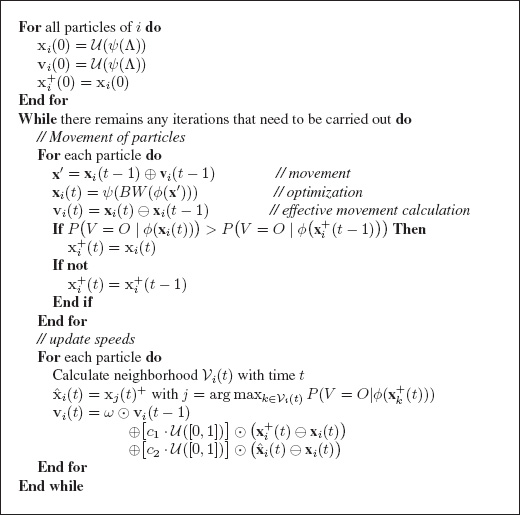
Algorithm 9.2. Adaptation of the PSO algorithm

Figure 9.4. An example of a circular neighborhood used in PSO

9.4.4. A behavioral comparison of the metaheuristics

The algorithms that have been mentioned in this section are based on metaheuristics which use other techniques that are used to explore different solution space. These metaheuristics are made up of a population of agents which interact with one another with the aim of being able to find the best solution possible. These agents interact with one another using different methods and different individuals and they do this at different times. The interactions which take place within a genetic algorithm are carried out by crossing the best quality solutions with one another and this is made possible by exchanging and sharing the genes of the solutions at each iteration of the algorithm. With this in mind, and if the codes of the adapted genes are present, it becomes possible for each iteration that occurs within the algorithm to transfer the best characteristics from the parent solutions to the child. In PSO the interaction of the different agents takes place at each iteration of the algorithm thanks to the updates of the velocity vectors. However, it is not possible to transfer the best characteristics of the particles such as the position of the particle. Instead of this, PSO looks for the best particles that exist within a particle’s neighborhood. The API algorithm uses an extremely different approach: the agents only interact with each other whenever the nest is moved. This type of interaction can be referred to as a direct interaction in the sense that the nest is a solution which is made available to each of the ants. Each of these approaches has its advantages and disadvantages. Interacting with each of the iterations, as is the case for the genetic algorithm and for the PSO algorithm, makes it possible to find the correct solutions in the quickest time possible. However, this frequency of interaction runs the risk of all of the agents moving in the same direction, which in turn reduces the diversity of the exploration process. In addition, if the agents find several similar solutions as far as the criterion of optimization is concerned, it becomes highly possible that poles of attraction will be created. This in turn means that the agents will only move between these poles and that any explorations that were carried out before the creation of these poles will be lost. However, it is sometimes necessary to concentrate the exploration efforts on several poles in order to guarantee the creation of an optimal or almost optimal solution. On the other hand, rare interactions can also occur and this is the case with the API algorithm. Such interactions can reduce the effectiveness of the search for an optimal solution since the research that is carried out is blind research, with no knowledge of the remaining solutions that are available. However, this rarity of interactions can also turn out to be advantageous because these rare interactions reduce the number of iterations that the agents need to consider before making a decision as to what pole they will move towards. The decision is made as soon as the nest is moved. This type of quick decision making can also turn out to be damaging in certain cases. In all of the examples that have been mentioned in this section, the moment when a decision is made (the interaction) can be an advantage or a disadvantage depending on the characteristics of the type of solutions involved. Hesitating between several solutions is better when we want to find the maximum optimal solution but this idea of hesitating between several solutions can reduce the speed at which the algorithm converges. The search for an optimal solution is carried out for each of the algorithms by a process of guided random research. In the case of the genetic algorithm, this search for the optimal solution is carried out by the mutation operator and in the case of the API algorithm it is carried out by the local exploration operator. These two different operators play similar roles. In the PSO algorithm the search for an optimal solution is carried out thanks to random contributions which come from the individual components of the algorithm whenever the velocity vectors are updated. In the genetic algorithm the search for an optimum solution is carried out by statistically reinforcing the zones that we are interested in exploring thanks to the use of the elitist selection operator. Each individual solution is part of the sample which is taken around the zone that we are interested in exploring. In the PSO algorithm the solutions are exploited by analyzing the spatial density of the particles which exist around the correct solutions. The exploitation of the solutions in the API algorithm is carried out by using two pieces of information: the position of the nest and the way in which the ants forage for food around a hunting site. These two mechanisms can be seen as a hierarchical reinforcement around the zones which we are interested in exploring. The nest determines the focal point around the zone, and around which the ants establish their hunting sites. The hunting site of an ant determines the zone in which it will search for its prey. The API algorithm has the capacity to do something which the other two algorithms are incapable of doing, which is that the API algorithm is able to forget about the exploration sites which proved to be unsuccessful. This is possible thanks to the API’s patience on the exploration sites and to its patience on waiting for the nest to be moved. The ability to do this is a huge advantage for the API algorithm since it can abandon a non-profitable zone and concentrate on another zone with the aim of not wasting any effort.

9.4.5. Parameter setting of the algorithms

The explanation of the experimental study that was carried out in relation to how these six approaches can be used to train a HMM is divided into two phases. The first phase involves carrying out a search for parameters on a reduced set of data. After this is complete, we will use the configurations of these parameters to evaluate the performance of the algorithms when they are applied to a bigger set of data.

DEFINITION 9.2. Let f_A,X be the probability distribution of the random variable which measures the performance of the algorithm A for a fixed configuration of X parameters. Let be Δ_υ=x = (∗, . . . , ∗, υ = x, ∗, . . . , ∗) the set of configurations of parameters for which the parameter v has a value x. The probability distribution f_A,Δυ=x is defined as:

A configuration X = (x₁, . . . , x_K) of parameters for a stochastic algorithm A is said to be strong, if for every value x_i, the probability distribution has a high mean and a reduced standard deviation.

Let EG = {(e₁, g₁), . . . , (e_L, g_L)} be a set of samples so that e_i is a configuration of Δ_υ=x parameters and g_i is the measurement of the configuration’s performance. The probability distribution f_A,Δυ=x can be approximated by the following probability distribution:

where (m, s) is the normal distribution of mean m and of standard-deviation s and considering the following equation:

Figure 9.5 shows the probability distributions which are the result of five different mutation rates which have been applied to the first image which can be seen in Figure 9.7 by using the AG-B algorithm.

Figure 9.5. Approximate distributions showing the probabilities of certain performances appearing, taking into consideration five different mutation rates for the AG-B algorithm

In order to determine the configurations of the strong parameters, we only need to compare the probability distributions. With the aim of carrying out a fair comparison of the algorithms, we have considered the configurations of parameters which provide the same opportunities to all the algorithms. Whenever the Baum-Welch algorithm is not used, the algorithms are able to evaluate approximately 30,000 HMMs (i.e. 30,000 uses of the forward algorithm). Whenever the Baum-Welch algorithm is used, the algorithms are able to carry out approximately 1,000 iterations of the Baum-Welch algorithm (2 or 5 iterations are carried out for each explored solution). The data that we have used for these experiments was obtained from images of faces taken from the ORL database [SAM 94]. The four faces which can be seen in Figure 9.7 are the faces that were used. These images are in 256 gray-level. We have recoded them into 32 gray-level and they have been linearized into gray-level sequences (see Figure 9.6).

Figure 9.6. The principle of coding an image into a sequence of observations with blocks of 10×10 pixels

Figure 9.7. The first faces of the first four people from the ORL image database [SAM 94]

Several different parameter settings have been taken into consideration for all of the conditions that have been mentioned above. The parameter settings that we obtained from the four images in Figure 9.7 are given in Table 9.2.

Table 9.2. The configurations of the parameters

9.4.6. Comparing the algorithms’ performances

In order to compare the algorithms with the configurations of the parameters, we decided to use four sets of images with each set of images being made up of between four and ten images. The characteristics of the sets of the images that were used can be seen in Table 9.3.

Table 9.3. Characteristics of the images used for programming the HMMs

In order to compare the effectiveness of the metaheuristics with a traditional approach we used algorithms Random0, Random2 and Random5. 30,000 HMMs were randomly chosen in the Λ solution space for algorithm Random0. The result of this algorithm is the best model that has been explored. For algorithms Random2 and Random5 we explored between 500 and 200 random HMMs. We then applied two or five iterations from the Baum-Welch algorithm to each random HMMs. We considered HMMs which had 10 and 40 hidden states.

Each image is transformed into a sequence by following the same principles that are used for setting the algorithms. The images are learned several times and the mean likelihood logarithm is computed. m(I, A) is the mean for an image I and for an algorithm A. If we note A as the set of algorithms that must be compared, then e(I, A) can be defined as follows:

The number e(I, A) measures the efficiency of algorithm A on a scale from zero to one for the image I. The most effective algorithm leads to e(I, A) = 1 and the least effective algorithm leads to e(I, A) = 0. In order to compare all of the algorithms with one another we suggest that the measurement ē(A) is used. Let be the set of images that are used. Then, we define:

Table 9.4 shows the results of the experiment. As we can see, the algorithms are divided into three groups. The first group is made up mainly of those algorithms which do not use the Baum-Welch algorithm. These algorithms tend not to perform as well as those algorithms which do use the Baum-Welch algorithm. We can also note that algorithm API-A1 provides worse statistics than if we were to carry out purely random research. It would seem that there is less chance of finding a good model by carrying out a poorly guided exploration of the different types of solutions than if a completely random exploration of the solutions were to be carried out. This example shows that it is necessary to carry out a comparative study of the metaheuristics if they are to be used to train the HMMs. The second group of algorithms contains those algorithms which have an average performance level (from 44.31% to 85.94%). The final group of algorithms contains the highest performing and the most effective algorithms. As we can see, these algorithms use two or five iterations from the Baum-Welch algorithm (but not all in the same way), and they search for HMMs in the Λ and Ω solution spaces. We can also see that as the performance of the algorithms increases and the lower the variability: their standard deviation decreases.

Table 9.4. A measurement of the algorithms’ efficiency

9.5. Conclusion

In this chapter we have discussed the problem of learning HMMs using metaheuristics. First of all, we introduced the HMMs and the traditional criteria that were used to train them. We also introduced the different types of solution spaces which are available nowadays, and which can be used to train the HMMs. The fact that there are different types of solution spaces available is a fact that is too often forgotten. The three types of search spaces that we investigated are complementary representations and include: a discrete representation (^T), a continuous representation (Λ) and a vector-space representation (Ω).

Our experiments have shown that there is less chance of finding a good HMM in the ^T solution space in comparison to the two other types of solution spaces, Λ and Ω; or at least this is the case with the search methods we used.

The use of metaheuristics for training HMMs has already been investigated and many encouraging results were found. In this chapter we introduced a comparative study which was inspired by three biologically-inspired approaches. Each approach focuses on a particular population of solutions. We have concentrated our comparison on one critical point, a point which can easily be analyzed and critiqued, i.e. the choice of parameters. We have tried to configure our algorithms in as fair a way as possible. However, we must bear in mind that the results and conclusions that we have obtained depend on the particular area of study that we chose to investigate, in other words, the training of sequences created from images whilst considering the maximum likelihood as the training criterion.

Our findings have also shown that a moderate use of a local optimization method (which in our case is the Baum-Welch algorithm) is in fact able to improve the performance of the metaheuristics that we chose to investigate.

The conclusions which can be drawn from this experimental study have led to new questions that need to be answered: is it possible to apply the results that we have found to other domains of study? Is it possible to apply the results to other criteria and to other metaheuristics? We strongly believe that it is best to act carefully when trying to answer such questions and to avoid too much generalization. We hope that this study can act as a framework for any future and more rigorous comparative studies.

9.6. Bibliography

[AGA 04] AGARWAL S., AWAN A. and ROTH D., “Learning to detect objects in images via a sparse, part-based representation”, IEEE Transactions on Pattern Analysis and Machine Intelligence, vol. 26, no. 11, pp. 1475–1490, 2004.

[AUP 05a] AUPETIT S., Contributions aux modèles de Markov cachés: métaheuristiques d’apprentissage, nouveaux modèles et visualisation de dissimilarité, PhD Thesis, Department of Information Technology, University of Tours, Tours, France, 30th November 2005.

[AUP 05b] AUPETIT S., MONMARCHÉ N. and SLIMANE M., “Apprentissage de modèles de Markov cachés par essaim particulaire”, BILLAUT J.-C. and ESSWEIN C. (Eds.), ROADEF’05: 6th Conference of the French Society of Operational Research and Decision Theory, vol. 1, pp. 375–391, François Rabelais University Press, Tours, France, 2005.

[AUP 05c] AUPETIT S., MONMARCHÉ N., SLIMANE M. and LIARDET S., “An exponential representation in the API algorithm for hidden Markov models training”, Proceedings of the 7th International Conference on Artificial Evolution (EA’05), Lille, France, October 2005, CD-Rom.

[BAU 67] BAUM L.E. and EAGON J.A., “An inequality with applications to statistical estimation for probabilistic functions of Markov processes to a model for ecology”, Bull American Mathematical Society, vol. 73, pp. 360–363, 1967.

[BAU 72] BAUM L.E., “An inequality and associated maximisation technique in statistical estimation for probabilistic functions of Markov processes”, Inequalities, vol. 3, pp. 1–8, 1972.

[BER 98] BERTHOLD M. and HAND D.J. (Eds.), Intelligent Data Analysis: An Introduction, Springer-Verlag, 1998.

[BUL 94] BULAJA S., Population-based incremental learning: a method for integrating genetic search based function optimization and competitive learning, Report no. CMU-CS-94-163, Carnegie Mellon University, 1994.

[BUL 95] BULAJA S. and CARUANA R., “Removing the genetics from the standard genetic algorithm”, in PRIEDITIS A. and RUSSEL S. (Eds.), The International Conference on Machine Learning (ML’95), San Mateo, CA, Morgan Kaufman Publishers, pp. 38–46, 1995.

[CAP 01] CAPPÉ O., “Ten years of HMMs”, http://www.tsi.enst.fr/cappe/docs/hmmbib.html, March 2001.

[CHE 04] CHEN T.-Y., MEI X.-D., PAN J.-S. and SUN S.-H., “Optimization of HMM by the Tabu search algorithm”, Journal Information Science and Engineering, vol. 20, no. 5, pp. 949–957, 2004.

[CLE 05] CLERC M., L’optimisation par Essaims Particulaires: Versions Paramétriques et Adaptatives, Hermes Science, Paris, 2005.

[DRE 03] DREO J., PETROWSKI A., SIARRY P. and TAILLARD E., Métaheuristiques pour l’Optimisation Difficile, Eyrolles, Paris, 2003.

[DUG 96] DUGAD R. and DESAI U.B., A tutorial on hidden Markov models, Report no. SPANN-96.1, Indian Institute of Technology, Bombay, India, May 1996.

[FOR 73] FORNEY JR. G.D., “The Viterbi algorithm”, Proceedings of IEEE, vol. 61, pp. 268–278, March 1973.

[GAN 99] GANAPATHIRAJU A., “Discriminative techniques in hidden Markov models”, Course paper, 1999.

[GIU 02] GIURGIU M., “Maximization of mutual information for training hidden Markov models in speech recognition”, 3rd COST #276 Workshop, Budapest, Hungary, pp. 96–101, October 2002.

[GLO 86] GLOVER F., “Future paths for integer programming and links to artificial intelligence”, Computers and Operations Research, vol. 13, pp. 533–549, 1986.

[GLO 89a] GLOVER F., “Tabu search – part I”, ORSA Journal on Computing, vol. 1, no. 3, pp. 190–206, 1989.

[GLO 89b] GLOVER F., “Tabu search – part II”, ORSA Journal on Computing, vol. 2, no. 1, pp. 4–32, 1989.

[GLO 97] GLOVER F. and LAGUNA M., Tabu Search, Kluwer Academic Publishers, 1997.

[GOL 89] GOLDBERG D.E., Genetic Algorithms in Search, Optimization and Machine Learning, Addison-Wesley, 1989.

[HAM 96] HAMAM Y. and AL ANI T., “Simulated annealing approach for Hidden Markov Models”, 4th WG-7.6 Working Conference on Optimization-Based Computer-Aided Modeling and Design, ESIEE, France, May 1996.

[HER 92] HERTZ A., TAILLARD E. and DE WERRA D., “A Tutorial on tabu search”, Proceedings of Giornate di Lavoro AIRO’95 (Enterprise Systems: Management of Technological and Organizational Changes), pp. 13–24, 1992.

[HOL 75] HOLLAND J.H., Adaptation in Natural and Artificial Systems, University of Michigan Press: Ann Arbor, MI, 1975.

[JUA 90] JUANG B.-H. and RABINER L.R., “The segmental k-means algorithm for estimating parameters of hidden Markov models”, IEEE Transactions on Acoustics, Speech and Signal Processing, vol. 38, no. 9, pp. 1639–1641, 1990.

[KAP 98] KAPADIA S., Discriminative training of hidden Markov models, PhD Thesis, Downing College, University of Cambridge, 18 March 1998.

[KEN 95] KENNEDY J. and EBERHART R., “Particle swarm optimization”, Proceedings of the IEEE International Joint Conference on Neural Networks, vol. 4, IEEE, pp. 1942–1948, 1995.

[KIR 83] KIRKPATRICK S., GELATT C.D. and VECCHI M.P., “Optimizing by simulated annealing”, Science, vol. 220, no. 4598, pp. 671–680, 13 May 1983.

[LJO 90] LJOLJE A., EPHRAIM Y. and RABINER L.R., “Estimation of hidden Markov model parameters by minimizing empirical error rate”, IEEE International Conference on Acoustic, Speech, Signal Processing, Albuquerque, pp. 709–712, April 1990.

[MAR 13] MARKOV A.A., “An example of statistical investigation in the text of “Eugene Onyegin” illustrating coupling of “tests” in chains”, Proceedings of Academic Scienctific St. Petersburg, VI, pp. 153–162, 1913.

[MAX 99] MAXWELL B. and ANDERSON S., “Training hidden Markov models using population-based learning”, BANZHAF W., DAIDA J., EIBEN A.E., GARZON M.H., HONAVAR V., JAKIELA M. and SMITH R.E. (Eds.), Proceedings of the Genetic and Evolutionary Computation Conference (GECCO’99), vol. 1, Orlando, Florida, USA, Morgan Kaufmann, p. 944, 1999.

[MON 00a] MONMARCHÉ N., Algorithmes de fourmis artificielles: applications à la classification et à l’optimisation, PhD Thesis, Department of Information Technology, University of Tours, 20th December 2000.

[MON 00b] MONMARCHÉ N., VENTURINI G. and SLIMANE M., “On how Pachycondyla apicalis ants suggest a new search algorithm”, Future Generation Computer Systems, vol. 16, no. 8, pp. 937–946, 2000.

[PAU 85] PAUL D.B., “Training of HMM recognizers by simulated annealing”, Proceedings of IEEE International Conference on Acoustics, Speech and Signal Processing, pp. 13–16, 1985.

[RAB 89] RABINER L.R., “A tutorial on hidden Markov models and selected applications in speech recognition”, Proceedings of the IEEE, vol. 77, no. 2, pp. 257–286, 1989.

[RAS 03] RASMUSSEN T.K. and KRINK T., “Improved hidden Markov model training for multiple sequence alignment by a particle swarm optimization – evolutionary algorithm hybrid”, BioSystems, vol. 72, pp. 5–17, 2003.

[SAM 94] SAMARIA F. and HARTER A., “Parameterisation of a stochastic model for human face identification”, IEEE Workshop on Applications of Computer Vision, Florida, December 1994.

[SAU 00] SAUL L. and RAHIM M., “Maximum likelihood and minimum classification error factor analysis for automatic speech recognition”, IEEE Transactions on Speech and Audio Processing, vol. 8, no. 2, pp. 115–125, 2000.

[SCH 97] SCHLUTER R., MACHEREY W., KANTHAK S., NEY H. and WELLING L., “Comparison of optimization methods for discriminative training criteria”, EUROSPEECH ’97, 5th European Conference on Speech Communication and Technology, Rhodes, Greece, pp. 15–18, September 1997.

[SLI 99] SLIMANE M., BROUARD T., VENTURINI G. and ASSELIN DE BEAUVILLE J.-P., “Apprentissage non-supervisé d’images par hybridation génétique d’une chaîne de Markov cachée”, Signal Processing, vol. 16, no. 6, pp. 461–475, 1999.

[TCD 06] “T.C. Design, Free Background Textures, Flowers”, http://www.tcdesign.net/free_textures_flowers.htm, January 2006.

[TEX 06] “Textures Unlimited: Black & white textures”, http://www.geocities.com/texturesunlimited/blackwhite.html, January 2006.

[THO 02] THOMSEN R., “Evolving the topology of hidden Markov models using evolutionary algorithms”, Proceedings of Parallel Problem Solving from Nature VII (PPSN-2002), pp. 861–870, 2002.

[VER 04] VERTANEN K., An overview of discriminative training for speech recognition, Report, University of Cambridge, 2004.

[VIT 67] VITERBI A.J., “Error bounds for convolutionnal codes and asymptotically optimum decoding algorithm”, IEEE Transactions on Information Theory, vol. 13, pp. 260–269, 1967.

1. Strictly, we should consider the hidden Markov model as the realization of a random variable and note P(V = O, S = Q | l = ). However, to simplify the notations, we have chosen to leave out the random variable which refers to the model.

2. The criterion of maximum likelihood is, nevertheless, the criterion that is used the most.