Chapter 13

Using Interactive Evolutionary Algorithms to Help Fit Cochlear Implants

13.1. Introduction

The surgical technique which enables profoundly deaf people with a fully functional cochlea to hear again was developed some 40 years ago [LOI 98]. During the surgical procedure, the surgeon inserts a very thin silicon filament which bears several electrode inserts, into the cochlea of the patients. The aim of this procedure is to stimulate the auditory nerve. The electrodes are connected to an antenna which is surgically placed under the skin, just behind the patient’s ear (see Figure 13.1).

In order to activate the electrodes, the patient wears a small apparatus called a BTE (for behind the ear) which looks like a hearing aid. The BTE is made up of two microphones that are connected to a digital signal processor (DSP) which transforms the received signal into electric pulses which are sent to the electrodes. The BTE is connected to a second exterior inductive antenna which works in collaboration with the antenna that is implanted under the patient’s skin, thanks to the use of a powerful magnet. The impulses that are emitted by the DSP are transmitted to the electrodes which have been implanted by the two inductive antennae (see Figure 13.1).

The objective of the interface that is created is to stimulate the auditory nerve with the aim of restoring the patient’s hearing to a certain level so that they are able to understand spoken language. The question of how to stimulate the auditory nerve is very important. It is tackled by adjusting the parameters of the DSP.

Figure 13.1. Principle of a cochlear implant: 1) microphone; 2) processor; 3) external antenna (fixed and centered by a magnet); 4) internal antenna inserted under the skin and containing a magnet; 5) electrodes inserted into the cochlea; 6) auditory nerve

The main problem is linked to the large number of parameters that need to be tuned, given that there are many causes for loss of hearing; for example, congenital deafness, traumatic deafness (due to an accident) or deafness due to illness. Other factors, such as the age of the patient, the number of years between the beginning of deafness and the implantation, the depth of insertion of the electrodes inside the cochlea, also add to this problem, making it very difficult to solve. The experience of the practitioners often leads to excellent results, such as patients who are able to follow a telephone conversation and enjoy listening to music. However, in some cases, no good results can be achieved for some unknown reason.

In this chapter, an interactive evolutionary algorithm is used to optimize the parameters of the DSP for patients for whom implantation is a failure.

This research was the doctoral thesis of Claire Bourgeois-République [BOU 04]. Further research has been carried out on her original research as part of the French Ministry of Health’s RNTS project known as HÉVÉA. This work was carried out at the ear, nose and throat department of Bobigny University Hospital in France.

13.1.1. Finding good parameters for the processor

The aim of adjusting the DSP’s parameters is to get the implant to fit the patient, and eventually enable him/her to distinguish between relevant information that is heard in speech in order to improve understanding. All of this should be possible without causing any discomfort to the patient, in other words it should be at an acceptable auditory level [LOI 00]. Originally, cochlear implants were only made up of one or two electrodes. In some cases this led to a vast and surprising improvement in the hearing of certain patients, despite the small number of electrodes. Thanks to the minimization process that exists nowadays, the designers of cochlear implants have been able to develop cochlear implants with 9, 15, 16, 20, 22 and even 24 electrodes [COC, MED, AB, MXM]. Results have been better than ever, but the number of parameters to be tuned has increased accordingly, along with the increased power of the embedded microprocessor.

The principal parameters which are available include the following:

– for each electrode:

- a range of sound frequencies which will activate the electrode,

- the minimum intensity threshold under which the patient will not be able to feel any sound sensation (referred to as T for threshold),

- the maximum intensity threshold which the patient can endure for a long period of time (referred to as C for comfort level);

– the number of electrodes which are activated simultaneously;

– the gain in hearing for each sound frequency;

– the sensitivity of the patient for each sound frequency;

– the use of one or two microcomputers;

– the type of stimulation chosen, etc.

In an implant which has 20 electrodes, there are easily hundreds of different parameters that need to be tuned, and that can have an important role when it comes to enabling the patient to understand everyday conversation.

13.1.2. Interacting with the patient

One important aspect that needs to be taken into consideration is the subjective nature of the interactions that take place with the patients. Evaluating the different parameters of the DSP and the cochlear implant depends on the patient being able to recognize different feelings, which can sometimes be quite difficult to express. Furthermore, evaluating the success of a cochlear implant can be quite biased. This is known as the Pygmalion effect, which means that patients tend to place surgeons and experts, who have years of experience in adjusting the fittings of the cochlear implants and DSP, on a pedestal because it is these people who enabled the patient to hear. As a result, the patients imagine that any adjustments made to the parameters of the DSP will be beneficial.

Then, there are often several sets of parameters which are available on the processor and which can be selected by a micro-switch that is located on the BTE worn behind the ear. It is common practice to refer to the current fitting as P1 and the previous fitting as P2 in case the most recently tested parameters are rejected by the patient (due to tiredness or lack of comfort, etc.). The possibility of moving from the old set of parameters to the new set also enables the patient to compare the two sets of parameters.

Currently, adjusting the parameters of the DSP and the cochlear implant takes place in the following way:

1) The fitting expert asks the patient if the last fitting was better or worse than the one carried out before that. The practitioner will then use the best recorded fitting as a basis from which he can start to work.

2) The expert then loads the fitting that needs to be improved (P1 or P2) into proprietary software to tune the implant.

3) The expert tries to find the problematic parameters, by carrying out a series of tests with the patient to check if the patient can recognize consonants, vowels and syllables.

4) Thanks to his experience, the expert then changes certain parameters and carries out the same tests to see if the adjustment which has been made has led to any improvement. This is where the Pygmalion effect usually comes in; if the adjustment has not worked or has had a negative effect on the patient’s hearing, the patient will often find it difficult to say so, mainly because he does not want to disappoint the expert. Another factor should also be taken into consideration: patients may have difficulties in communicating, since, after all, it should not be forgotten that these patients are profoundly deaf. The age of the patients also varies.

5) The previous point is repeated until the expert and the patient are both satisfied with the adjustments that have been made.

6) The previous best fitting is loaded into the P2 memory and the new fitting to be tested is loaded into the P1 memory.

It takes between 45 mins and 1 hour to find new satisfactory parameters. Then, the patient has to evaluate the new fittings over a period of several weeks in order to take neuro-plasticity into consideration. If the patient is not satisfied with the new fitting after this period of several weeks, another appointment will be made so that the fitting can be adjusted again. In some cases, evaluating the patient’s ability to understand spoken language is carried out by speech therapists in hospital. If this is the case, evaluation normally takes longer than 1 hour.

Computer scientists who are specialized in optimization will see a problem in the protocol which has been described above: the optimization which is carried out is a type of local research. The expert who adjusts the fittings of the cochlear implants tries to improve on the best fitting that has been found to date. The expert will use this best fitting as his basis and will only change some of the parameters in order to improve them. This means that the new fitting will be very similar to the previous one. If the problem is multimodal, then the expert runs the risk of becoming trapped by a local optimum and the patient’s hearing will never get better.

13.2. Choosing an optimization algorithm

The process that was described in the previous section is long and does not look like it can be optimized with an algorithm.

However, an actual discussion with a patient led to the possibility of such an optimization taking place. The patient said that he was capable of immediately detecting if the new fitting was good or not. However, we still cannot count on thousands of evaluations to find the best possible fitting, so a deterministic algorithm could not be used. Among stochastic algorithms, we must find one that will not be much affected by local optima, but that is still able to converge quite rapidly in order to improve obtained results within a limited number of evaluations.

Figure 13.2. The evolutionary loop

Evolutionary algorithms (see Figure 13.2) have experienced a significant development and growth since their revival at the beginning of the 1990s:

1) An initial population is created and then evaluated (by a user in the case of an interactive algorithm) with the aim of creating a population of parents.

2) If we are not satisfied (non-verified stopping criterion), then n parents are selected (from the best parents) to create m children with the help of genetic operators.

3) The new individuals who are created are then evaluated.

4) Finally, the weakest individuals are eliminated thanks to the use of a replacement operator. This phase makes it possible to reduce the size of the population to its initial size. The loop is restarted at point two with a new generation of parents.

The use of evolutionary algorithms has become increasingly widespread in many different domains and their increased use towards the end of the 1990s means that they are much better understood now. As a result, it has become possible to use them to solve different interactive problems [COL 04], as can be seen in the work published by Takagi [TAK 98, TAK 99, TAK 01] and by [HER 97, BIL 94 DUR 02]. Rwo approaches can be used to reduce the number of evaluations: the Parisian approach [COL 00] (described in Chapter 2 and which dramatically reduces the number of evaluations) or Krishnakumar’s micro-GAs [KRI 89] that use populations of a few individuals only. In his tutorials on evolution strategies, Thomas Bäck shows that it is possible for evolution strategies to produce better results than human experts for a number of evaluations of the same order than the number of real parameters that need to be optimized [BAE 05].

These recent results have shown that the theories which suggested that evolutionary algorithms were to be used when all else failed, and required tens of thousands of evaluations in order to produce an average result, are no longer valid. A well designed evolutionary algorithm can now find interesting solutions with a reduced number of evaluations. Evolutionary algorithms seem to be more suited to solving multimodal problems than other stochastic methods such as simulated annealing, even if there are only a few individuals in the population. In the next sections of this chapter it is assumed that the reader possesses some knowledge of standard evolutionary algorithms (for an introduction to this topic it is recommended that the reader looks at [DEJ 05]). The descriptions that are given for this type of algorithm will also highlight any changes that have been made to them when they are to be used interactively.

13.3. Adapting an evolutionary algorithm to the interactive fitting of cochlear implants

In an interactive evolutionary algorithm it is the human user who evaluates each individual that is suggested by the algorithm. As far as the optimization of the parameters of a cochlear implant is concerned, it is the patient who evaluates the fitting of the implant based on a particular series of words or syllables. It is therefore not possible to rely on a large number of evaluations, because in a domain like this fatigue, as well as the physiological and physical behavior of the patient, can also influence the results.

According to Thomas Bäck’s results [BAE 05], an evolutionary algorithm should perform as well as, if not better, than a human expert on a number of evaluations equivalent in size to the number of real parameters that need to be optimized. Therefore, 100 evaluations would allow an EA to perform better than a human on a problem with 100 real parameters. If it is possible to reduce the evaluation time for each parameter from 45 minutes down to only 5 minutes, then it would take 8 hours to complete the evaluation of the 100 parameters, which is not unreasonable over two days. Knowing that the presented work only optimizes 30 parameters, we can hope to do better than a human expert during a two day fitting session.

It is also necessary to take certain psychological aspects into consideration. For example, if the convergence speed of the algorithm is correctly tuned for the 100 evaluations, (i.e. 8 hours to carry out the fitting), then the patient could be disheartened by this because over 8 hours progression would be very slow. The idea is then to break the experiment into several partial optimizations and have some “restarts” [JAN 02].

Doing this also brings another advantage: all optimization algorithms (including Eas) have a strong tendency to converge prematurely on local optimae, meaning that optimizers usually implement many techniques to delay the convergence of the algorithm. If several restarts are used, convergence is, on the contrary, no longer a problem. In interactive evolution, we want an algorithm to converge very quickly, so that the patient sees an improvement over the very few evaluations of one run, and keeps up his spirit. After several restarts, we can use the best individuals of the previous runs (which will hopefully have converged on different solutions) as the initial population of afinal fitting session.

So, rather than fighting against premature convergence, this work will encourage it (by using a micro-GA, for instance).

13.3.1.Population size and the number of children per generation

There are two possibilities which arise on a fixed number of evaluations: either we choose to create many children per generation over a few generations, or we create a few children per generation over many generations.

Of these two possibilities, the latter will most favor convergence. This means that a steady-state type of replacement will be used (or a (μ + λ) replacement strategy, with a heavily reduced λ (number of children) [BAE 95]). Then, in order to avoid using too many evaluations in the initial population, the population size can be reduced as in micro-GAs [KRI 89].

Now, as far as the optimization of cochlear implants is concerned, there are too many parameters to hope to optimize them all. Fitting experts have recommended starting with the optimization of the minimal T and maximum C thresholds for each electrode, meaning two variables per electrode. For MXM cochlear implants which have 15 electrodes, this means that 30 real variables need to be optimized over 100 evaluations, giving good chances of performing better than a human expert.

13.3.2. Initialization

There is one major constraint that needs to be respected: the maximum value for the stimulation of each electrode (C value) must never be exceeded, so as not to damage the patient’s auditory neurons. For each new patient, the first appointment with the fitting expert consists of a “psychophysical” test in order to determine this maximum level for each electrode. A minimum intensity level (T value) is also determined because if an electrode is stimulated under this intensity level it means that a patient would be unable to hear anything.

Then, the initialization of each individual is carried out by taking two random values within the predetermined [T, C] interval for each electrode.

13.3.3. Parent selection

Parent selection is different from parent replacement (see section 13.3.5) in that a parent can be selected several times.

A 0.9 stochastic tournament [BLI 95] is used, that chooses 2 parents at random, and returns the better of the two with a 90% probability. This selection is preferred to a proportional selection that would rely on the fitness landscape of the problem (which is unknown here).

13.3.4. Crossover

The genome is made up of real values, which means that it could have been possible to use some type of barycentric crossover. However, since the aim is to make the intervals evolve, adopting this style of crossover would actually have progressively reduced the width of the intervals.

Therefore, the method used for crossovers comes from binary genetic algorithms. Genes are exchanged between parents after a particular crossover point (the locus, chosen at random) has been reached. A single-point crossover is used because according to experts, we can expect a high level of epistasis between the different electrodes. Using multi-point crossover points would therefore have been disruptive and would have turned the crossover into some kind of macro-mutation.

Determining the locus is carried out electrode by electrode in the hope of not breaking any good combinations of genes that exist, meaning that T and C values are not separated. Since the evolutionary algorithm is a (μ + λ) type of algorithm, with a number of children that is smaller than the population size (see Figure 13.2., crossover is therefore used for the creation of each child (100% probability).

13.3.5. Mutation

Mutation is also used with a 100% probability level on each child that has been produced by the crossover process. In the evolutionary algorithm, each gene has a 10% probability of being mutated. Since there are 30 genes, each child will undergo three mutations on average. These figures may seem high but due to the high level of epistasis that exists, modifying one threshold on a genome would have a limited effect on the general evaluation process. This high rate of mutation lets the algorithm keep some kind of exploratory character, despite the low number of evaluations that take place.

13.3.6. Replacement

A steady-state like replacement is used, in order to promote fast convergence. However, where a strict steady-state would create only one child that would replace the worst of the parents, several children will be created, turning this replacement operator into a kind of (μ + λ) replacement, even though the number of children is very small.

13.4. Evaluation

Until now, evaluating a patient’s ability to understand speech has been the test for a new fitting. The first method involved sending the patient back home with the new fitting stored in the P1 memory and the previous fittings stored in the P2 memory. This meant that the patient was able to compare the two different fittings in his own environment. The other method involved a speech therapist who carried out an evaluation on the patient using intensive tests taking over one hour to complete.

However, it was impossible to apply an interactive evolutionary algorithm with any of these two methods since the evaluation time was much too long. A new evaluation protocol was developed using calibrated sentences taken from Professor Lafon’s cochlear lists [LAF 64] that contain syllables that are both representative of the French language and supposed to be discriminant cochlear-wise. Ten sentences (a total of 78 words) were chosen to evaluate a patient’s understanding of the French spoken language. Here are the sentences (with their translation, even though their meaning is clearly secondary):

Maximizing the understanding of a patient is, of course, one of the main objectives of the evaluation process but it must also be comfortable enough for patients to use in their everyday life.

The overall evaluation is therefore the weighted mean of the comfort level of the cochlear implant (marked over 10) and of the patient’s understanding. For the tests which are described in the next section, the comfort mark is multiplied by 2.2 which means the overall comfort mark is out of 22. The total number of words that were recognized (out of 78) is added to this mark in order to get a total overall mark of 100. This total mark out of 100 will be used as the patient’s evaluation for the evolutionary algorithm. Understanding has the predominant mark, while comfort is not totally ignored.

The evaluation procedure typically lasts about four minutes. Four minutes is clearly not long enough to obtain a precise evaluation of a patient’s ability to hear/understand speech, but it enables us to carry out 100 tests in 6h40′, or 1h20′ per run, if the 100 evaluations are divided into 5 runs. The aim of this reduced evaluation protocol is different from the complete evaluation protocol which is carried out by experts. Since experts cannot test as many configurations as evolutionary algorithms (patients may only have as many as ten appointments in one year) they need to work on as precise as possible evaluation of their patient’s hearing.

Evolutionary algorithms work in a different way. They are stochastic processes that test many different fittings. They do not need very precise evaluations of the results, but need to be roughly guided towards a good solution. In fact, getting only a rough estimation of the patient’s hearing may improve the efficiency of the algorithm, as it may help to skip over local optima.

13.5. Experiments

A certain number of experiments were carried out, which led to surprising results in many respects. The first set of experiments described in the next part of this section was carried out by Claire Bourgeois-République as part of her doctoral thesis at the University of Bourgogne and was published in several articles [BOU 04, BOU 05a, BOU 05b]. Other, more recent, tests were carried out as part of the RNTS HÉVÉA project which was supported by the French Ministry of Health.

13.5.1. The first experiment with patient A

The first experiment using the algorithm mentioned in the previous section was carried out with a patient whose hearing became progressively worse until the patient became totally deaf in 1983. In 1991 the patient was first implanted with a one-electrode implant in the right ear. This implant was later replaced with a 15-electrode MXM implant, which was activated by an external processor the size of a walkman that clipped to the belt. The MXM implant with 15 electrodes led to average results. In 2003, the same patient then bought a behind the ear (BTE) miniaturized processor. As its name suggests, this miniaturized processor is worn behind the ear. However, the results were not as good as the results of the walkman-style processor, so the patient decided to stop using the BTE processor.

13.5.1.1. Psychophysical test

The psychophysical test (which is used to determine the CT and C thresholds for each electrode) was performed by an expert practitioner (see Table 13.1). Electrodes 10, 11 and 12 were not functional (the patient was unable to hear anything regardless of the power of the stimulation) and therefore not activated.

Table 13.1. The set of T and C parameters

13.5.1.2. Evaluation of the expert’s fitting with the BTE and the hearing aid

Before the experiments were started, the best fittings previously obtained by the expert after 10 years on the walkman processor and BTE processor were tested against the 4-minute evaluation function that will be used for the evolutionary algorithm.

As a reference point, the weighted mark for the walkman processor is 53/100, whereas the weighted mark for the BTE is 48.5/100. These marks confirm the patient’s observation: the BTE performs worse than the walkman-size processor.

All the experiments below are done with the BTE processor.

13.5.1.3. Experiment 1 and results

The aim of this first set of experiments was not to actually obtain good results, but to tune the parameters of the algorithm (determining the optimal size of the population, the number of children per generation, the selection pressure, etc.. Successive tests were then carried out on the algorithm with the aim of varying these parameters.

The first test uses a population of three individuals, with three children produced per generation. This test also uses a stochastic tournament selection with a probability of 0.8. The mutation rate of each parameter is fixed at 0.1 and the crossover rate of each parameter is fixed at 1.

During this first experiment, 12 different fittings were evaluated by the patient. Evaluating one fitting (preparation and evaluation) lasts a little less than four minutes. The results which were obtained for this experiment can be seen in Table 13.2.

Table 13.2. Results of experiment 1

The first line refers to the number of particular fittings to be evaluated and the second line refers to the fitting’s weighted mark. There are three fittings per generation, so fittings 1 to 3 refer to the first generation, fittings 4 to 6 to the second generation, and so on.

The first three evaluations correspond to the individuals which were part of the initial population and which were created randomly. The process of artificial evolution begins at fitting 4. Fitting 5 has a mark that is higher than the expert’s best fitting. Fittings 7 and 8 have almost identical parameters and have identical marks. The algorithm seems to converge from the fitting 10 onwards with a very good mark of 81. The patient is happy and appreciates the speed of the evaluation procedure.

13.5.1.4. Experiment 2 and results

For this second experiment, the number of individuals of the population and the number of children per generation are doubled with the aim of delaying the premature convergence that was observed in experiment 1. The initial population is therefore increased to six individuals and four children are produced per generation.

Table 13.3. Results of experiment 2

The marks of the first six individuals are generally low. However, what is rather surprising is that one of the six random individuals (i.e. one of the first six fittings) has a mark which is higher than the mark obtained by the expert (53 vs 48.5). As can be seen in Table 13.3, the genetic operators are unable to find any suitable individuals. This is why the algorithm is stopped voluntarily after fitting 17, for the well-being of the patient. Results are not as good and the patient becomes increasingly tired.

13.5.1.5. Experiment 3 and results

During this experiment the population is reduced again to three individuals and only two children are produced per generation. In order to prevent any premature convergence (as was the case during experiment 1), mutation rate is increased to 0.6. A roulette-wheel type of selection is then tested. This type of selection is tested as it may have a stronger selection pressure on a problem where fitness varies a lot between individuals.

Table 13.4. Results of experiment 3

From the first three individuals that were created randomly (fittings 1 to 3), the first shows once again a mark that is slightly higher than the mark obtained by the expert. Table 13.4 shows that the marks of the individuals steadily increase. From the fitting 5 onwards, all of the marks are higher than 50. The best individual is the fitting 16 which has a mark of 73.

13.5.1.6. Experiment 4 and results

For the fourth experiment, the size of the population is four individuals and four children are produced per generation. The mutation rate is 0.1 and the selection mode used for choosing the parents is once again tournament selection.

Table 13.5. Results of experiment 4

Table 13.5 shows that the individuals that were randomly chosen from the population (fittings 1 to 4) achieve an average mark of 59.5 (this mark is much higher than the mark of 48.5 that was achieved for the BTE by the expert, even after many years). All the other values are above 56.5. The best marks from this experiment and from all of the experiments are 91 and 91.5, and were achieved by the 14^th and 15^th individuals respectively (in other words more than 90% of the words from Professor Lafon’s list were understood). The patient is extremely happy and is astonished by such good results.

13.5.1.7 Experiment 5 and its results

The size of the population is fixed at five individuals and two children are produced per generation. The selection mode which is used to choose the parents is, once again, a tournament selection and the mutation rate is 0.1.

Table 13.6 shows that two out of the five individuals which make up the initial population (fittings 1 to 5) achieve marks above 70. However, because of the evolution of the algorithm, it is impossible to find one particular individual which is better than the rest. The algorithm is stopped during the evaluation of the 23^rd fitting.

Table 13.6. Results of experiment 5

13.5.2. Analyzing the results

Figure 13.3 shows how the value of the best individual evolves during the evaluation process, which takes place in each experiment. As far as evolution is concerned, experiments 1, 3 and 4 led to the best results (there was an increase in the marks obtained by each individual). The good number of individuals to have in a population seems to be 3 or 4. The good number of children to have per population is quite low (2 or 3). These values validate the hypotheses that were made earlier in this section.

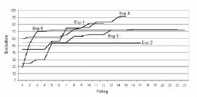
Figure 13.3. Evolution of the best individual during the evaluation processes which were carried out for each experiment

Medically speaking, it seems rather strange that the random fittings (the initial population) would yield better results than the results obtained by the expert practitioner. Some explanation is given below on this particular point.

The T and C values of the best and worst individuals have been plotted for each electrode in Figure 13.4. The dark lines refer to the minimum and maximum values given by the psychophysical test (see section 13.5.1.1). The dotted curve refers to the T and C values of the worst fitting, and the thin lines refer to the best fitting (with a mark of 91.5).

Figure 13.4. T and C values of the best and worst fittings

The medical team, and in particular the experts who specialize in cochlear implants, were surprised that this particular fitting was the best because of the small [T,C] intervals observed for electrodes 3, 4, 5, 6, 12, 14 and 15 (0; 0.5 and 1). Usually, the expert generally tries to feed the auditory nerve with maximum information, and therefore tries to maximize the [T,C] interval for each electrode. This means that the expert usually sets the T and C values to the same values as those that are determined during the psychophysical test. The expert might sometimes reduce these values if he has the feeling that too much information may saturate the auditory nerve, but this happens rarely. In this case, the interactive evolutionary algorithm minimized the values of C-T for practically all the electrodes except 1, 7, (8) and 9, which does not make much sense. Nevertheless, doing this enabled us to obtain better results than if all the C-T values had been maximized (the expert’s fittings).

Several issues therefore arise:

– is minimizing the [T,C] interval equivalent to de-selecting an electrode?

– would there be a problem of interference between the electrodes (diaphony)?

– would the problem be combinatorial (i.e. would certain combinations of electrode work better than others)?

13.5.3. Second set of experiments: verifying the hypotheses

A second set of experiments was then carried out, with fittings that were not created by the interactive evolutionary algorithm, but were created in order to validate certain hypotheses. The tests were carried out with the same patient and with the same evaluation protocol.

It should be pointed out that a period of one month elapsed between the two tests. During this one month break, the patient went back to using his old walkman-style processor, meaning that he was therefore unable to physiologically adapt to any new fittings (neuroplasticity). This means that the evaluations of the two experiments can therefore be compared with one another. In the next part of this section the first set of experiments will be referred to as C1 and the second set of experiments will be referred to as C2.

13.5.3.1. Experiment 7: is the minimization of C-T equivalent to de-selecting an electrode?

For this experiment all of the electrodes apart from electrodes 1, 7 and 9 are reduced to intensities which are much lower than the liminary intensities (T). This means that the patient will not hear anything from these electrodes.

However, the differences between T and C have been maximized for electrodes 1, 7 and 9 (see Figure 13.5).

Figure 13.5. Experiment 7

The resulting weighted mark of this fitting is 82, with a level of understanding of 90%. In other words, the patient was able to understand 90% of the words from Professor Lafon’s sentences. This fact alone seems to confirm three points:

1) Minimizing the difference of C-T is equivalent to de-selecting electrodes, since similar results were obtained as for the best individual.

2) This fitting (which can be compared to the best fitting that was evaluated a month earlier) still produces a good result.

3) All of the electrodes, apart from electrodes 1, 7 and 9 (which were maximized) have been minimized in order to produce a good result. The problem thus seems to be quite binary (even if the values of each interval were refined, it would only lead to a slight improvement as far as the quality of the result is concerned).

13.5.3.2. Experiment 8: a study of electrode 8 and its influence on the fitting

In the C1 set of experiments, the evolutionary algorithm set a medium interval on electrode 8. In this test, electrode 8 was maximized along with electrodes 1, 7 and 9, using the values from the psychophysical test.

The resulting weighted mark of this fitting is 81. The patient finds that the fitting is slightly less comfortable than the previous fitting, although the level of understanding is exactly the same. Electrode 8 seems to play a rather neutral role as far as understanding spoken language is concerned.

13.5.3.3. Experiment 9: is there any diaphony between the electrodes?

In order to investigate this hypothesis, the even-numbered electrodes are deactivated (both T and C are set to a value below the T liminary intensity) and the odd-numbered electrodes are maximized (by using the values from the psychophysical test). The aim of this action is to increase the spacing between active electrodes (see Figure 13.6).

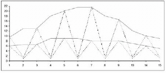
Figure 13.6. Experiment 9

The resulted weighted mark of this fitting is 78.8. The patient stated that this fitting was less comfortable than the others. This result is obviously not as good as the results that were obtained for experiments 7 and 8. Adding other electrodes to electrodes 1, 7 and 9 does not seem to improve the fitting. The result, however, is still better than the expert’s result of 48.5 that was obtained for the BTE.

13.5.3.4. Experiment 10: a wider spacing of the electrodes

In order to further decrease the risk of interference, in this experiment we decided to activate one in every three electrodes instead of every two electrodes. Electrodes 7 and 9 remained activated and the maximized electrodes are now electrodes 1, 4, 7, 9, and 15 (electrodes 10 to 12 are non-functional); see Figure 13.7.

The result is astonishing. The fitting is not very comfortable and the weighted mark for this fitting is only 58.5. First of all, these facts refute the idea that interference between the different electrodes could exist, but above all, if maximized electrodes are compared with those of experiment 7 (where only electrodes 1, 7 and 9 were activated), the difference being the addition of electrodes 4 and 15.

This information suggests that this binary problem is combinatorial. In other words, there are certain combinations of electrodes that work better than others. Another conclusion which can be drawn from these facts is that the activation of certain electrodes has a negative effect on a patient’s understanding of spoken language (adding electrodes 4 and 15 degraded speech understanding).

Figure 13.7. Experiment 10

13.5.3.5. Experiment 11: evaluation of the best individual from C1

Experiment 11 investigates the reliability and accuracy of the evaluation protocol.

The parameters of the best fitting from the C1 set of experiments (with a mark of 91.5), which were carried out a month earlier, are tested once again.

The result of the vocal test is once again very good (94% of the words are understood), and even slightly better than one month earlier, but the fitting is evaluated as slightly less comfortable, which accounts for a weighted mark of only 86.2. This mark is slightly lower than the previous weighted mark of 91.5, but it is still the best fitting that was found during the C2 set of experiments.

13.5.3.6. Experiment 12: an evaluation of the expert’s fitting

For this experiment the original expert’s best fitting (in which more or less all of the electrodes were maximized, and which obtained a mark of 48.5 during the C1 set of experiments) is uploaded into the BTE.

The result of the vocal test is poor (only 33% of the words were understood), and the comfort mark, which was given by the patient, was only 4/10. This means that the weighted mark this time was only 41.8, a mark which is much worse than that obtained during the C1 set of experiments.

In the period of one month, the best fitting generated by the interactive evolutionary algorithm went from a mark of 91.5 to 86.2, and the expert’s fittings went from a mark of 48.5 to 41.8. The absolute values have decreased between C1 and C2, but the difference remains about the same (43 against 44.4). Repeating these two fittings showed that the quick evaluation procedure is pretty reliable, because results are reproducible after one month, during which the patient used his old processor (and therefore could not adapt to other settings).

13.5.3.7. Other experiments

In order to check whether the evolutionary algorithm actually added some value, other tests were performed with randomly chosen values for T and C. Results were average to poor (but often higher than 41.8, the expert’s best fitting) and comfort was often criticized by the patients. The fact that many random fittings obtained better results than the expert’s fitting may be explained by the fact that by maximizing the [T,C] interval of all electrodes, the expert also maximizes the influence of detrimental electrodes such as electrode 4 for the tested patient. By doing so, if there is only one detrimental electrode for a patient, the expert is sure to obtain a relatively bad speech understanding result, while a random fitting that would skip detrimental electrodes would very likely perform better.

13.5.4. Third set of experiments with other patients

One thing stands out from the previous results: in several cases the random values for the T and C parameters gave a result which was equal to or better than the expert’s best fitting (who understandably was trying to maximize the [T,C] interval for all of the electrodes).

A new series of tests was then started with four other patients in order to confirm or refute this observation. Unlike the previous experiments (where the evaluation process was a very short process with only ten sentences taken from the Lafon corpus), auditory speech evaluation (ASE) tests and vowel consonant vowel (VCV) recognition tests were used. The test is longer, but it makes it possible to determine a patient’s hearing ability in a much more detailed manner.

It would take too long to provide a complete summary of the tests in this chapter. The results of the tests are shown as percentages of recognized VCVs in Table 3.7.

Table 13.7. Results of tests shown as percentages of recognized VCVs

In almost all cases, if three random fittings are tested, it is nearly always possible to find a result that is equal to or better than the expert’s fitting.

In the final case (patient D), another marking system was used. This marking system was based on the ASE test. For this patient the best fitting that was obtained by the expert can be seen in Figure 13.8. The mark corresponds to the psychophysical test in which the intervals for each electrode are maximized.

In this experiment the evolutionary algorithm was briefly tested (only six evaluations due to the time that was required to complete the evaluations) and the best individual obtained an ASE mark of 22/22 (in comparison to a mark of 20.5/22 for the fitting which was set by the expert). Once again there were some astonishing values that were recorded for the electrodes (see Figure 13.9).

Given the very low number of evaluations, it is not possible to consider the algorithm as having played an important role in achieving such a result. However, analyzing the results is quite interesting because the intervals for all of the electrodes are quite small. Some of the electrodes were deselected and these included electrodes 5, 8, 11, 12 and 13. This goes against the recommendations of the experts and the developers of cochlear implants, who have been working in this field since the development of cochlear implants first took place over 40 years ago. However, once such electrodes have been removed, this supports the observation made by the first patient who had a better understanding of spoken language when only 3 out of the 12 electrodes were activated.

Figure 13.8. The best fitting obtained by the expert for patient D: each rectangle represents the [T, C] interval for each electrode

Figure 13.9. The best individual for patient D: each rectangle represents the [T, C] interval for each electrode

13.6. Medical issues which were raised during the experiments

It should be pointed out that our study does not focus on a wide range of different cases and because of this the results cannot be used on a more general level. However, throughout our study certain issues have been raised and we think it would be interesting to try and find a solution to such issues. As far as the first set of experiments is concerned, they were all carried out on only one patient.

1) In studying the graphs which show the progression of the different evolutionary tests, and which also show the results produced from the second set of tests, it is possible to evaluate a patient’s hearing (with the help of an optimization algorithm) in less than four minutes. This fact alone goes against the recommendations made by speech therapists. Speech therapists believe that it is impossible to evaluate a patient’s hearing in less than 20 minutes.

The speech therapists are, of course, correct. They are correct in the sense that a four minute evaluation will not lead to the same quality of conclusions as a one-hour evaluation. However, in pragmatic terms, an evaluation procedure must be used in relation to the quality of the optimization algorithm that is also used. An evolutionary algorithm does not benefit from any of the experience or intelligence that an expert has. The quality of a very refined evaluation process (and therefore long evaluation) would be wasted if such a rough algorithm were to be used.

Therefore, for such algorithms, it is better to have more evaluations than more precise evaluations. A more refined and longer evaluation process would benefit a human expert who works in this field, since the expert is able to provide a better interpretation of the results from the tests and therefore provide a better evaluation of a patient’s hearing.

2) Patient D seems to be able to evaluate a new fitting within seconds. However, experts say that a patient can only give a true evaluation of any new fitting at least one or two weeks after the new fitting has been installed (this is probably due to neuroplasticity).

Once again, the experts are more than likely correct if the aim is to carry out a more detailed evaluation of the patient’s hearing. As far as a rough evaluation is concerned (which is fine for an evolutionary algorithm) it is not problematic to evaluate the fitting only seconds after it was uploaded in the processor (but one example may not be enough to generalize this conclusion).

3) With patient D it was possible to carry out 89 tests with different parameters, in a period of one and a half days, with results that were good enough to guide an interactive evolutionary algorithm where speech therapists and other experts working in this field believe that after a period of two hours any evaluations that are carried out are no longer relevant, due to patient fatigue. The same comments as above may apply here.

4) With two patients, it has been possible to obtain a similar or higher level of understanding of spoken language when some of the electrodes were either minimized or deselected where experts, as well as cochlear implant manufacturers, believe that it would make more sense to maximize the number of activated electrodes and to maximize their range of stimulation.

This point still remains a mystery and requires further investigation in order to provide a more accurate explanation.

On a less general note, it seems that for patient A the problem is combinatorial, i.e. certain combinations of electrodes work better than others. This can be seen in the example where two electrodes (electrodes 4 and 15) were added to a set of electrodes (1, 7 and 9). With this particular combination of electrodes, the patient’s understanding of the spoken language actually got worse. If this hypothesis were proved, it would lead to a big problem, because:

a) the problem would face a combinatorial explosion. With nine electrodes, the number of possible combinations is 2⁹ = 512. With 15 electrodes, the number of possible combinations is 2¹⁵ = 32,768, and with 22 electrodes, the number of possible combinations is a massive 2²² = 4,194,304;

b) since the expert has no way to determine which electrode will have a positive or negative effect on speech understanding this means that, in theory, it would be necessary to test all electrode combinations in order to find the best combination. This, however, is impossible in practice.

As far as the third set of tests is concerned, it seems that one in every three random parameters taken from the T and C thresholds leads to a result that is equal to, if not better than the result which is obtained by the expert (who maximizes the [T,C] intervals). This point alone suggests that there are numerous fittings that are satisfactory for the patient.

13.7. Algorithmic conclusions for patient A

To start with, the contribution of the implemented evolutionary algorithm seems to be real, looking at Figure 13.3, even though it might seem surprising to achieve such good results in such a short period of time. However, if the problem is combinatorial (where certain combinations of electrodes enable a patient to understand spoken language better), then the chances of finding a good combination whilst using an interactive evolutionary algorithm for 100 evaluations are far from being zero:

1) in the case of patient A, three electrodes out of 15 were non-functional. This means that out of the remaining 12 activated electrodes, there were a total of 2¹² = 4.096 different combinations of electrodes;

2) if we assume that there are over 100 random evaluations, then the chances of finding the correct combination is one in 40;

3) as is suggested in the random tests carried out during the third set of experiments, it is possible for different combinations of electrodes to carry out a good evaluation. If there are ten satisfactory combinations, then 100 random evaluations would have one chance in 4 of finding one of these ten good combinations;

4) it should not be forgotten that having one chance in 4 of finding a good combination (using 100 evaluations) is obtained solely by random research.

If it is assumed that an evolutionary algorithm can perform better than a random search, the probability of finding a good fitting suddenly comes closer to 1. However, all of this is only possible if the algorithm is capable of carrying out many evaluations in a short period of time.

Finally, there is one final element that changes the probability of finding a good fitting from “very probable” to “extremely probable”: the interactive evaluation given by the patient may be of very high quality, and this is very important because evaluation is what guides the evolutionary algorithm. During the 15^th French evolutionary workshop (JET) organized by the French Society for Artificial Evolution, a competition was organized with the aim of solving the famous MasterMind board game. This was a very difficult task to complete because the problem was a 13 × 13 size problem (13 positions, 13 colors), meaning that it was necessary to find a good combination from among 3.10¹⁴, i.e. approximately 300 thousand billion. On 1,000 games, the best evolutionary algorithm was able to find the correct combination in an average of only 19.5 evaluations.

This feat was only possible because the information given by the MasterMind game’s evaluation function is very rich (number of correct colored pegs in the correct place, and number of correct colored pegs in incorrect places), and that the evolutionary algorithm found a way to exploit it correctly.

As far as cochlear implants are concerned, if the interactive evaluation that is given by the patient is of high quality, then this could significantly simplify the problem. All works on interactive evolutionary algorithms seem to support this idea [TAK 05].

Furthermore, micro-population evolutionary algorithms have also proved to be efficient [KRI 89], and the number of variables to optimize was lower than the number of available evaluations. This set of hypotheses seems to reinforce the idea that the good results were not obtained through chance.

The only way it is possible to confirm this would be to carry out a significant number of complete tests with new patients.

13.8. Conclusion

Fitting a cochlear implant is a problem for which it is very difficult, if not impossible to find a suitable solution deterministically within a limited time period for at least two reasons:

– the objective function cannot be modeled and can vary a lot due to the fact that it is dependent on the patient and linked to the subjective evaluation of his sensations;

– the search space is large enough to eliminate any guarantee of optimality.

The work and the findings that are presented in this chapter describe a way to help the expert practitioner by using a micro-population interactive evolutionary algorithm. The first tests are very promising and the results raised several issues related to the current evaluation protocol that is used by experts in the field. The results also seem to question the seemingly evident idea that more electrodes would allow the patient to understand better, and that maximizing the [T,C] interval of all electrodes may not be a good idea, if for a patient some electrodes are detrimental to speech understanding.

However, it goes without saying that this work is only the beginning. It is now necessary to build on this research by carrying out numerous clinical experiments.

13.9. Bibliography

[AB] Advanced Bionics: http://www.cochlearimplant.com

[BAE 95] BAECK T., Evolutionary Algorithms in Theory and Practice, New-York, Oxford University Press, 1995.

[BAE 05] BAECK T., “Tutorial on evolution strategies”, Genetic and Evolutionary Computation Conference Gecco’05, 2005.

[BIL 94] BILES J., “GenJam: a genetic algorithm for generating jazz solos”, Proceedings of the International Computer Music Conference, San Francisco, 1994.

[BLI 95] BLICKLE T., THIELE L., “A mathematical analysis of tournament selection”, ESHELMAN L. J., (Ed.), Proceedings of the 6^th International Conference on Genetic Algorithms, Morgan Kauffmann, p.9-16, 1995.

[BOU 04] BOURGEOIS-RÉPUBLIQUE C., Plateforme de réglage automatique et adaptatif d’implant cochléaire par algorithme évolutionnaire interactif, PhD Thesis, University of Bourgogne, France, 2004.

[BOU 05a] BOURGEOIS-RÉPUBLIQUE C., FRACHET B., COLLET P., “Using an interactive evolutionary algorithm to help with the fitting of a cochlear implant”, MEDGEC (GECCO), 2005.

[BOU 05b] BOURGEOIS-RÉPUBLIQUE C., VALIGIANI G., COLLET P., “An interactive evolutionary algorithm for cochlear implant fitting: first results”, SAC, p. 231-235, 2005.

[COC] Cochlear: http://www.cochlear.com

[COL 00] COLLET P., LUTTON E., RAYNAL F., SCHOENAUER M., “Polar IFS + Parisian GP = efficient inverse IFS problem solving”, Genetic Programming and Evolvable Machines, vol. 1, number 4, p. 339-361, 2000.

[COL 04] COLLET P., Vers une évolution interactive, from his thesis and Habilitation à Diriger des Recherches, June 2004, University of the Littoral Côte d’Opale.

[DEJ 05] DEJONG K., Evolutionary Computation: a Unified Approach, MIT Press, 2005.

[DUR 02] DURANT E. A., Hearing aid fitting with genetic algorithms, PhD Thesis, University of Michigan, USA, 2002.

[EA] The Association for Artificial Evolution: http://ea.inria.fr.

[HER 97] HERDY M.,“Evolutionary optimization based on subjective selection – evolving blends of coffee”, Proceedings of the 5^th European Congress on Intelligent Techniques and soft Computing, EUFIT’97, 1997.

[JAN 02] JANSEN T., “On the analysis of dynamic restart strategies for evolutionary algorithms”, Parallel Problem Solving from Nature, p. 33-43, 2002.

[KRI 89] KRISHNAKUMAR K., “Micro-genetic algorithms for stationary and non-stationary function optimization”, SPIE: Intelligent Control and Adaptive Systems, vol. 1196, Philadelphia, PA, 1989.

[LAF 64] LAFON J., “Le test phonétique et la mesure de l’audition”, Ed. Centrex, Eindhoven, 1964.

[LOI 98] LOIZOU P., “Introduction to cochlear implants”, IEEE Signal Processing Magazine, p. 101-130, 1998.

[LOI 00] LOIZOU P., POROY O., DORMAN M., “The effect of parametric variations of cochlear implant processors on speech understanding”, Journal of Acoustical Society of America, p. 790-802, 2000.

[MED] MEDEL, http://www.medel.com

[MM] Mastermind competition: http://tniyurl.com/gaa7y

[MXM] MXM Labs: http://www.mxmlabs.com

[TAK 98] TAKAGI H., “Interactive evolutionary computation: system optimization based on human subjective evaluation”, Proceedings of the IEEE Intelligent Engineering Systems (INES’98), Vienna, Austria, 1998.

[TAK 99] TAKAGI H., OHSAKI M., “IEC-based hearing aid fitting”, Proceedings of the IEEE Conference on Systems volume 3, 1999.

[TAK 01] TAKAGI H., “Interactive evolutionary computation: fusion of the capabilities of EC optimization and human evaluation”, Proceedings of the IEEE, Vol.89, number 9, 2001.

[TAK 05] TAKAGI H., “Tutorial on interactive evolutionary algorithms”, 2005.