Chapter 3

Wavelets and Fractals for Signal and Image Analysis

3.1. Introduction

The determination of singularities and of scaling laws by multifractal analysis (which uses multiresolution techniques based on the concept of wavelets) can be found in more and more applications in the fields of natural science, engineering and economics.

In this chapter we highlight the different multifractal methods by analyzing 1D and 2D generic signals; the self-similarity of fractals using wavelet transform modulus maxima has allowed scientists to determine the distribution of the singularities of the very different complex signals which can be found in the domains of material physics, biology and medicine.

The different themes in the chapter have been chosen for their relevance in relation to the further improvements and advances in scientific know-how as well as for the improvement in the quality of results that have been obtained during scientific experiments. The aim of including these themes is to help the reader better understand and apply certain purely mathematical theories which are normally difficult to carry out.

3.2. Some general points on fractals

They exist everywhere around us. These luminous, unusual, beautiful shapes are known as fractals.

3.2.1. Fractals and paradox

It is not easy to give a correct definition of fractals. Nevertheless, in terms of etymology the word fractal leads us to the idea of fractus meaning irregular or broken shape [MAN 82].

The analysis of unusual mathematical objects such as curves of infinite length, which possess a finite area, or non-derivable continuous functions, has considerably developed thanks to the work carried out by Mandelbrot, the founder of fractal geometry.

We can see fractal geometry around us in our everyday lives, in nature, in biology or in physics. Generally speaking, the term fractal is used for mathematical objects whose shape and complexity are governed by the inherent omnipresence of irregularities.

The scale invariance and the self-similarity of an object or signal must be taken into consideration in order to facilitate the exploration of fractals. An object is said to be scale-invariant when it is left unchanged following expansion; it is thus symmetric for this transformation process. Consequently, this property means that the change in the observation scale does not change the statistics which have been calculated from the signal. In other words, the general shape of the object remains the same regardless of the change in scale.

Unlike a Euclidean geometric figure, a fractal does not possess any scale or any characteristic of size. Each portion of the fractal reproduces the general shape of the signal regardless of the scale enlargement: this is the property known as self-similarity. This idea means that the information which comes from observation of the fractal is independent of the resolution at which the fractal’s measurement is taken.

Fractal analysis was borne from the need to have a tool which could be adapted to the study of complex and irregular natural or artificial phenomena.

For the most part, the recent success of (multi)fractal analysis in the optimization of signal and image processing does not stem from the fact that the signals which are studied are fractal. In reality, and with some rare exceptions, the signals do not possess any self-similarity nor any attributes which are normally associated with fractal objects (except the idea of irregularity on all scales). The development of the methods used in fractal analysis enables scientists to describe the structure of the singularity of complex structures in fine detail. The development of these methods has also enabled scientists to study models which are the result of fractal analysis and which have led to significant progress in areas such as turbulence, growth models, finance, vibration phenomena, material rupture, biomedical signals, satellite images, earthquakes, etc.

3.2.2. Fractal sets and self-similarity

A set A ⊂Rⁿ Ris said to be self-similar if the combination of unrelated sub-sets A₁ ,...A_k can be obtained from A by expansion, translation and rotation. This notion of self-similarity often implies an infinite multiplication of points, which leads to the creation of irregular structures. The Von Koch curve and Cantor’s triadic set are simple examples of these irregular structures.

DEFINITION 3.1.– Let f be a signal with compact support A. A signal f is self-similar if unrelated sub-sets A₁ ,...A_k exist, so that the restriction of the graph of f to each point A_i is an affine transformation of f. Thus a scale of s_i > 1, a translation u_i, a weight P_i and a constant c_i exist, so that

It is assumed that f is constant when it is outside these sets.

Figures 3.2 and 3.4 illustrate that if f is self-similar then its wavelet transformation is also self-similar.

3.2.2.1. The Von Koch snowflake

The Von Koch curve was published in an article in 1904 which was entitled: “On a continuous curve without tangents, constructible from elementary geometry”, [VON 04]. The Von Koch curve is a fractal set which is obtained by recursively dividing a segment of length l into four segments of length l/3 as can be seen in Figure 3.1. The length of each subdivision is then multiplied by 4/3. The limit of this process of subdivision thus results in a curve with infinite length.

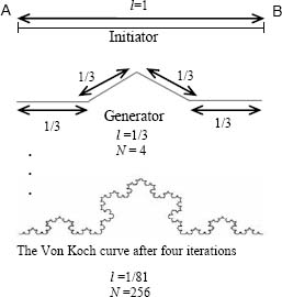
Figure 3.1. Some iterations of a subdivision of Von Koch curve. The Von Koch curve is a fractal which is the result of an infinite number of subdivisions

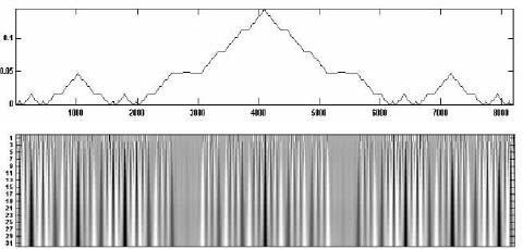
Figure 3.2. The analysis of the Von Koch curve by wavelet transformation with ψ = − θ′ where θ is a Gaussian function shows self-similarity

Wavelet analysis detects the singularities of the signal and shows the initial pattern of the signal on a fine scale. This initial pattern is identically reproduced over and over again.

3.2.2.2. Cantor’s set

The triadic set, introduced by Georg Cantor in 1884 [CAN 84], is created by recursively dividing intervals of size l into two intervals l/3 and a central hole, as can be seen in Figure 3.3. The triadic set which is the result of the limit of the subdivisions of the intervals is a set of points known as Cantor’s set.

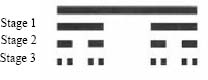
Figure 3.3. Three iterations using Cantor’s set

Figure 3.4. The analysis of the Cantor set signal by wavelet transformation with ψ = −θ′ where θ is a Gaussian function shows self-similarity

3.2.3. Fractal dimension

Determining the dimension is to establish the relationship between the way in which an object uses its space, and its scale variation.

We tend to attribute whole dimensions to Euclidean geometric shapes: straight lines, circles, cubes, etc.

Fractals possess complex topological properties, for example the Von Koch snowflake, which is of infinite length but which resides in a finitely sized square. Faced with these difficulties, Hausdorff came up with a new definition of dimension, which was based on the variations of the size of the sets during the change in scale. This idea became the basis of his fundamental work in 1919 [HAU 19], which was developed further in 1935 by Besicovitch [BES 35].

3.2.3.1. Some definitions

The fractal dimension (sometimes called the capacity dimension) can be defined as follows.

DEFINITION 3.2.– Let A be a bounded part of Rⁿ and N(s) the minimum number of balls of radius s which are necessary to cover A, then the fractal dimension can be defined as follows: .

The measurement of A is . The measurement of A can be either finite or infinite.

With this formula it is possible to identify the idea of the box-counting dimension which is very useful in certain applications (see Figure 3.6).

Another definition which can be attributed to Hausdorff-Besicovitch gives a new perspective on the Hausdorff-Besicovitch dimension

DEFINITION 3.3.– The Hausdorff-Besicovitch dimension d_H-B is defined as the logarithmic quotient of the number of internal homothetic transformations N of an object, by the inverse proportion of this homothety (1/s):

EXAMPLES 3.1

– For a point:

– For a segment, it is possible to establish two internal homothetic transformations of ratio 1:2:

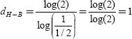
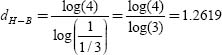
– For the Von Koch snowflake:

At each iteration and from each side, four new similar sides are generated in a homothetic ratio of 1:3.

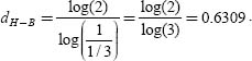
– For Cantor’s triadic set

At each iteration the current intervals are divided into two smaller intervals and a central hole in a homothetic ratio of 1:3.

– For the following fractal curve:

Figure 3.5. Calculation of the Hausdorff-Besicovitch dimension from any given fractal

NOTE 3.1.– The fractal dimension of the Von Koch curve is not equal to its unit size as is the case for all traditional linear geometric shapes. In the case of Cantor’s set, the limit of its subdivisions is a set of points in an interval [0,1]. Therefore, the Euclidean dimension of a point is zero whilst the fractal dimension of this set is 0.63.

As a consequence, the fractal dimension is greater than the topological or Euclidean dimension.

EXAMPLE 3.2.– The following application gives some insight into the principal use of the box-counting method by using linear regression to calculate the fractal dimension of a curve which represents a given physical phenomenon:

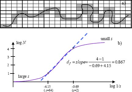
Figure 3.6. Calculation of the fractal dimension by linear regression. (a) Paving followed by the covering of the function by N boxes of size s; (b) evolution of log (N) vs log (1/s)

EXAMPLE 3.3.– Estimation of the fractal dimension from rupture profile using the Fraclab toolbox.

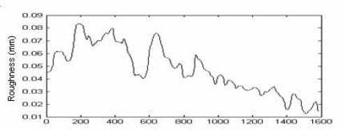
Figure 3.7. Rupture profile¹

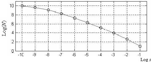
Figure 3.8. Estimation of the fractal dimension using box-counting method d_f = 1.0082

Some software for calculating the fractal dimension:

1. Matlab FRACLAB toolbox (free);
2. FDC (Fractal Dimension Calculator);
3. HarFA (Harmonic and Fractal image Analyzer);
4. BENOIT Fractal Analysis System;
5. FRACTALYSE.

3.3. Multifractal analysis of signals

The objective of multifractal analysis is to describe and analyze phenomena whose regularity, which is measured by a particular indicator (the Hölder exponent), can vary from one point to another. Thus, multifractal analysis provides both a local and global description of a signal’s singularity; a local description is obtained using the Hölder exponent, and the global description is obtained thanks to multifractal spectra. The multifractal spectra geometrically and statistically characterize the distribution of singularities which are present on the signal’s support.

3.3.1. Regularity

EXAMPLE 3.4.– The Weierstrass function: self-similarity and singularities

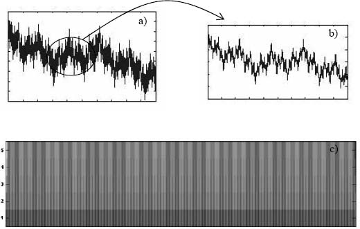
Figure 3.9. A signal generated by the Weierstrass function where α = 0.9 and β = 0.3: (a) the complete signal; (b) an extraction from a part of this signal; (c) its WT modulus

The signal , in which α and β are real numbers and α, is odd (under the condition 0 < α < 1 < αβ), is a continuous signal which is non-derivable. Its Hölder function is constant. Figure 3.9(b) shows the self-similarity of the signal; the shape of the signal remains the same regardless of the scale of the representation used. Figure 3.9(c) represents the wavelet transform modulus of f(t) which is calculated from a wavelet which has been derived from a Gaussian style wavelet: in other words confirming this notion of self-similarity on all scales and also confirming the detection of singularities (presence of impulses).

3.3.1.1. The roughness exponent (Hurst exponent)

Rough surfaces, which can be the result of a rupture, may lead to invariance through anisotropic transformation (self-affinity). In this case the surfaces are described by a local roughness exponent or by the Hurst exponent which verifies that: ∀ x = (x, y) R² in a neighborhood of x₀, ∃H R such that, for all values of λ > 0 :

In the case of a random phenomenon the symbol ~ signifies equality in terms of the laws of probability.

The Hurst exponent always has a value between zero and one and characterizes the fluctuations of height in a given surface. The analyzed surface might possess some properties of self-affinity meaning that it possesses properties of isotropic scale invariance if δ=1 or of anisotropic scale invariance if δ≠1.

3.3.1.2. Local regularity (Hölder exponent)

Local regularity is introduced with the aim of describing the signals that show signs of local fluctuations, in this case, the Hurst exponent is insufficient when it comes to determining the regularity of the signals. A signal is said to be regular if it can be approached locally by a polynomial.

A signal is said to be a regular Hölder signal h(x₀) ≥ 0 if there is the presence of a polynomial P_x0 and a constant C > 0, so that:

If f can be differentiated n times in the neighborhood x₀, then P_x0 is equal to the Taylor series of f at x₀.

If 0 ≤ α < 1, then the regular part of f(x) is reduced to P_x0 (x) = f (x₀) and therefore

The Hölder exponent provides a measurement of the rugosity of f(x): the closer the value of f(x) is to one then the softer its trajectory will be. The closer the value of f(x) is to zero, then the more variability the trajectory or the surface will possess. This increased variability corresponds to an increased level of rugosity. Singularities play a fundamental role in the study of signals and they often carry essential and relevant information. In the case of an image, its contours correspond to discontinuities or sudden variations in grayscale. These discontinuities or sudden variations in grayscale are the pieces of information that are recorded by a singularity of scale h.

EXAMPLE 3.5.– The calculation of the Hölder exponent of the profile of a rupture surface of an elastomeric material: characteristics of rugosity.

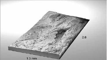
Figure 3.10. A 3D representation of one of the rupture surfaces of an elastomeric material

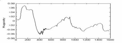
Figure 3.11. Example of a rupture profile

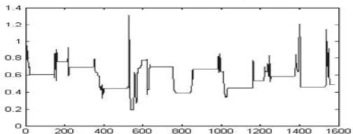
Figure 3.12. The values of the local Hölder exponent calculated for each point of the profile

INTERPRETATION 3.1.– Our signal describes a profile (Figure 3.11) which has been extracted from a rupture surface of an elastomeric material that can be seen as a 3D representation in Figure 3.10. The calculation of the local Hölder exponent of this signal was created with the help of the Fraclab toolbox.

Figure 3.12 shows that the majority of the values of the local exponent are between zero and one, with some peak values above one, reaching a maximum of 1.3. The most notable point of this graph peaks at an amplitude of 1.3 for an abscissa of 552. This value of 1.3 is characterized by a sharp increase in h (the Hölder exponent) and is followed by much smaller values of 0.3. The most singular points of the entire profile, i.e. those with the smallest exponent, can be found straight after the maximum value of 1.3. The value of the exponent is approximately 0.25 for an abscissa of between 555 and 570; in other words this means that there is a strong level of rugosity of the rupture’s surface. This interval relates to the breaking point of the material and can correspond to a default or inclusion in the surface of the rupture.

Our analysis remains basic and our objective is to trace the causes of the ruptures, for example by carrying out research into the defects which cause the material to break, or by looking at the poor physical and chemical design of the material. This study shows that the evolution of the local Hölder exponent provides clear and relevant information during the propagation analysis of cracks in a given material.

3.3.2. Multifractal spectrum

It is important to determine the distribution of the singularities of a multifractal in order to analyze its properties. The singularity spectrum (noted as D(h) and defined as the Hausdorff dimension of points where the Hölder exponent carries a particular value (iso-Hölder sets)) provides a geometric description of the singularities and measures the global distribution of the different Hölder exponents.

Mathematically, this can be defined as follows [MAL 98].

DEFINITION 3.4.– Let A_h be the set of all the points where the punctual regular Hölder signal of a multifractal is worth h. The singularity spectrum D(h) of a multifractal is the fractal dimension (the Hausdorff dimension) of A_h. The support of D(h)is the entire sets of h for which A_h is not empty.

Consequently, according to the definition of the fractal dimension given in section 3.2, covering the support of a multifractal by unconnected intervals of size s gives the number of intervals which intersects A_h:

The singularity spectrum thus expresses the proportion of singularities h which appear on a given scale s. The singularity spectrum of multifractals can easily be measured from the wavelet transform modulus which will be introduced in section 3.4.4.

NOTE 3.2.– A multifractal is said to be homogenous if all of its singularities have the same Hölder exponent h = α0, the support of D(h) therefore become punctual {α₀}.

The multifractal approach of 2D signals enables scientists to consider light intensity as a measurement of local information held by the image [LEV 00, LEV 97, LEV 94, LEV 92, BER 94].

A Hölder exponent is attributed to each point x on the image h = h(x) according to the following equation:

This equation provides information on the local regularity of the image in a neighborhood of x. Once this simulation has been carried out on the entire image it is then possible to construct sets of regularities by grouping together the points of the image which have the most similar Hölder exponent values in order to measure the Hausdorff dimension of these sets, noted as d_H. The pair (h, d_H), which is then obtained, can be used as an important piece of information in different applications:

– detection of contours; the contours of an image are identified with the component that is linked to the strongest singularities;

– measurement of the rugosity of a texture;

– denoising.

A large part of the noise (pixels of isolated singularities which do not correspond to any contour) can be eliminated by carrying out threshold techniques which are based on the notion of dimension.

Figure 3.13 shows an example of the multifractal spectrum of a rupture surface image as well as the corresponding contours.

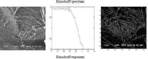
Figure 3.13. Estimation of the exponents of the singularities of the rupture surface. On the left: the original image of the face. Center: distribution of the values of the image’s singularity exponents. On the right: grayscale representation of the singularity exponents: the clearer the pixel, the weaker the exponent of the pixel

Despite the complexity of the texture of the image, this method ensures the detection of very fine contours.

3.4. Distribution of singularities based on wavelets

3.4.1. Qualitative approach

Singularities and irregular structures of a signal carry relevant information. It is very important to detect and characterize the discontinuities in the intensity of pixels which describes an image. This intensity also defines the contours of a scene (Figure 3.13) or the transient of a pathological electro-encephalogram.

In order to characterize singular structures, it is necessary to quantify the regularity of the signal f(t). The Hölder exponent (sometimes also referred to as the Lipchitz exponent) provides the measurements for uniform regularity of intervals as well as for any given point v. If f is singular, i.e. non-derivable, its behavior is described by the Hölder exponent.

The decrease of the wavelet transform modulus according to the respective scale is linked to the global and punctual regularity of the signal. Measuring this asymptotic decrease can be compared to “zooming” into the structures of a signal with a scale that tends towards zero.

3.4.2. A rough guide to the world of wavelet

In the case of an image, the “time-scale” or “space-scale” analysis is based on the use of a very extensive range of scales used to analyze a signal. This type of analysis is often referred to as a multiresolution analysis. Multiresolution analysis is based on a variety of different behaviors in terms of the laws that define the scales (e.g. rather large to very fine scales). The different scales are used to “zoom” into the structure of the signal and obtain increasingly precise representations of the signal that is being analyzed. A function ψ(t) or a localized and oscillating wave known as “mother-wavelet” are needed for the operation named above.

The condition of localization implies a rapid decrease when |t| increases indefinitely and the oscillation suggests that ψ(t) vibrates just as a wave does and that ψ(t)’s average and its n moments equal zero:

This property (n vanishing moments) is important in order to analyze the local regularity of a signal. Indeed, the Hölder regularity index increases with increasing the number of vanishing wavelet moments. Furthermore, the wavelet is (a zero average function) centered around zero with a finite energy.

The mother-wavelet ψ(t) – whose scale, based on a convention, is 1 – generates other wavelets ψ_u,s(t), s > 0, u R. This generation of other wavelets is based on the changes of the scale s as well as on temporal translation u:

ψu,s(t) is therefore centered around u.

The wavelet transform of f, expressed by Wf(u,s), for the scale s and the position u, is calculated by correlating f with the corresponding wavelet:

where ψ^*u,s describes the complex conjugate of ψ_u,s.

In a way, this transformation measures the fluctuations in a signal f(t) around a specific point u and for the scale provided by s > 0. This type of property has interesting applications and allows for the detection of transients and analysis of fractals. These transients are detected when zooming all along the scales and fractal analysis in determining the distribution of singularities.

It is possible to compare the time-scale analysis (u, s) to a time-frequency representation (u, η/s) where ψ_u,s is symbolically represented by rectangles whose dimensions vary according to s. Their surface, however, remains the same (Figure 3.14). This idea therefore also represents the Heisenberg uncertainty principle:

respectively represents the temporal resolution (or standard deviation) and the frequency resolution.

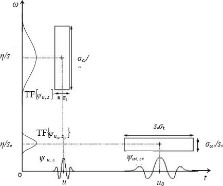
Figure 3.14. Process of wavelet analysis and the illustration of the Heisenberg uncertainty principle

Figure 3.14 shows that if s decreases, the frequency support increases and shifts towards higher frequencies. As a result the temporal resolution improves.

Figures 3.15(a) and (b) show some examples of wavelets that are very useful in the analysis of signals.

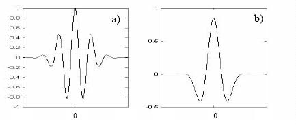
Figure 3.15. Wavelets generated from a Gaussian function θ;(a) Morlet: θ modulated; (b) Mexican hat: -θ″

3.4.3. Wavelet Transform Modulus Maxima (WTMM) method

Wavelet ψ is assumed to have n moments equal to zero. This wavelet is also Cⁿ with the derivates of a rapid decrease. This means that for every 0 ≤ k ≤ n and m N, there is C_m such that:

Jaffard’s necessary and sufficient condition [JAF 91] on wavelet transform, used in order to estimate the Hölder (or Lipchitz) punctual regularity of f at a point v, can be expressed as follows:

if f L²(R) is Hölder² α ≤ n, there exists A such that:

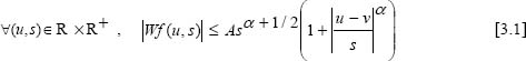
Based on what has been discussed above, the Hölder local regularity of f at v depends on the decrease of |Wf(u,s)| at fine scales in the neighborhood of v. The decrease of |Wf(u,s)| can indeed be controlled by the values of its local maxima.

Modulus maximum describes any point (u₀, s₀) such that |Wf(u₀, s₀)| is locally maximum at u = u₀ [OUA 02]. This implies:

NOTE 3.3.– The singularities are detected by searching the abscissa where the wavelet modulus maxima converge at fine scales. Indeed, if ψ has exactly n moments equal to zero and a compact support, there is θ with a compact support such that ψ = (–1)n θ⁽ⁿ⁾ with . The wavelet transform can be expressed as a multiscale differential operator of order n: with .

If the wavelet has only one moment which equals zero, wavelet modulus maxima are the maxima of the first order derivate of f smoothened by . These multiscale modulus maxima are used for the location of discontinuities as well as when analyzing the contours of an image. If the wavelet has two moments that equal zero, the modulus maxima correspond to large curvatures.

NOTE 3.4.– A contrario, if Wf(u,s) does not have a local maximum on the level of fine scales, then f is regular in that local area.

NOTE 3.5.– In general nothing guarantees that a modulus maxima is situated at (u₀, s₀) nor that this modulus is part of a line of maxima that propagates finer scales. However, in the case of θ being a Gaussian function, the modulus maxima of Wf(u,s) belong to the related curves that are never interrupted when the scale decreases.

NOTE 3.6.– In the case of an image, the points of the contours are distributed on curves that often correspond to the boundaries of the main structures. The modulus of individual maximum wavelets are linked to form a curve of maxima that follows the outline. For an image, partial derivates of wavelets linked to x₁ and x₂ of a smoothing function θ are also taken into consideration.

Function θ is assumed to be localized around x₁ = x₂ = 0 and isotropic (does not depend on |x|). The Gaussian function and the Mexican hat wavelet are wavelets that meet these requirements. The corresponding wavelets transform is as follows:

where * describes the operator of the convolution product.

This transformation can equally be expressed by its modulus |Wf(u,s)| and its argument Arg{Wf(u,s)}.

This signifies that the 2D-wavelet transform defines the gradient field of f(x) smoothened by θ. Note that the gradient indicates the direction of the largest variation of f for a smoothened scale s and that the orthogonal direction is often referred to as the direction of maximum regularity.

Furthermore, in the sense of Canny’s detection of the contours, wavelet modulus maxima are defined by the respective points u where |Wf(u,s)| is a local maximum that tends towards the direction of the given gradient described by the angle Arg{Wf(u,s)}. Its points create a chain that is referred to as the maxima chain. They might also be referred to as a gradient vector that indicates the local direction in which the signal varies the most when compared to the smoothened scale s.

The skeleton of wavelet transformation consists of two lines of maxima that are convergent up to the point of plane (x₁, x₂,) in the limits of s → 0. This skeleton carries out the positioning of the space-scale that contains all information concerning the fluctuations of the local regularity of f.

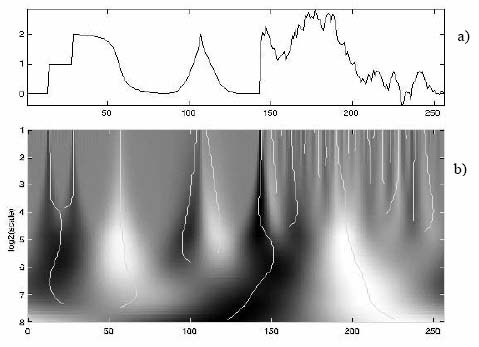
Figure 3.16. (a) Signal f(t )shows its singularities; (b) the wavelet modulus maxima and the lines of maxima of this modulus

Figure 3.16 can be accessed on the website http://cas.ensmp.fr/~chaplais/ and shows that the singularities create coefficients of great amplitude in their cone of influence. WTMMs detect the singularities well and allow us to estimate graphically the order of singularity of f (t) at all times in representing the WTMM linked to the function of the scale s. The gradient (based on the hypothesis of linearity) of the curve, e.g. log-log, obtained at a specific point in time, provides an estimation of the Hölder coefficient.

NOTE 3.7.– Numerical aspects. It is well known that derivatives of Gaussians are used to guarantee that all maxima lines propagate up to the finest scales. However, the process of chaining maxima must be performed with caution due to the apparition of artefacts in areas where the wavelet transform is close to zero.

Moreover, the finest scale of the wavelet transform is limited by the resolution of data. Then, the sampling period must be sufficiently small so that α is measured precisely.

3.4.4. Spectrum of singularities and wavelets

The singularities of multifractals vary from one point to another. It is important to establish the distribution of these singularities to analyze their properties. In practice, the distribution of singularities is estimated by global measurements which use self-similarities of multifractals. In this way, the fractal dimension of the points with the same Hölder regularity is calculated. The function used for this calculation is a function based on global partition calculated on the basis of the WTMM. The self-similarity of the wavelet transform modulus leads to the positions of the values of wavelet transform modulus maxima being equally self-similar.

In practice, the spectrum of singularities written as D(α) or D(h) for multifractals is measured based on the local maxima of the wavelet transformation.

Let ψ be a wavelet with n vanishing moments. If f has pointwese Hölder reglarity α₀ < n at v, the wavelet transform Wf(u,s) possesses a set of modulus maxima that are convergent towards v at fine scales.

All maxima at the scale s can be interpreted as a recovery of the singular support of f by wavelets of scale s. For its maxima, the following applies:

Let represent the positions of all local maxima of |Wf(u,s)| on a fixed scale s, [α_min, α_min] is the support of D(α), and ψ a wavelet with n > α_max moments equal to zero. The calculation of the spectrum D(α) for a self-similar signal f is carried out as follows:

– calculation of maxima; determine Wf (u,s) and its modulus maxima for each scale s; create chains of the wavelets’ maxima across scales;

– calculation of the function of partition (measurement of the sum of power q for these wavelet modulus maxima)

– determination of the scaling exponent τ(q) by linear regression of log₂ Z(s,q) as function of log₂s

Note that the Hölder exponent α and the spectrum of singularities D(α) are conjugated variables of q and τ(q). This means that D(α) can be obtained by inverting the Legendre transform of τ(q) under the hypothesis that D(α) is convex;

– determination of the spectrum

NOTE 3.8 – The monofractals or the homogenous fractals are characterized by a single Hölder exponent h (or α) = H (the Hurst exponent) of a spectrum τ_q which is linear and whose gradient is given by . On the other hand, a non-linear behavior of τ_q indicates a multifractal for which the Hölder exponent h(x) is a variable.

3.4.5. WTMM and some didactic signals

Highly oscillatory signals

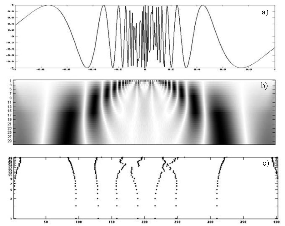
Figure 3.17. (a) Signal f (t) = sin(a/t); (b) the modulus of its wavelet transform calculated with ψ = −θ′ where θ is a Gaussian function; (c) the lines of maxima for this modulus

Figure 3.17 shows the analysis of a generic signal which is highly

oscillatory and discontinuous at t = 0. If (u, s) is in the cone of influence of 0, condition [3.1] is verified for α = h = 2. However, Figure 3.17 shows that there are coefficients for wavelets of high energy outside the cone of influence centered at 0. The instantaneous frequency of f(t) is , and if u varies, the set of points (u,s(u)) describes a parabolic curve situated outside the cone of influence centered around 0. The WTTMs confirm that large amplitudes are situated outside the cone of influence.

A signal with a finite number of discontinuities

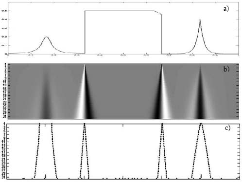
Figure 3.18. (a) signal f(t) with a finite number of discontinuities; (b) its wavelet transform modulus calculated with ψ = −θ″ where θ is a Gaussian; (c) the lines of maxima for this modulus

Figure 3.18 represents the analysis of a generic signal which shows singularities that are marked by discontinuities and non-derivabilities. The WTTMs are calculated with the help of a wavelet which is a second derivative of a Gaussian. The decrease of |Wf(u,s)| described by s is expressed throughout several curves of maxima. These curves correspond to the smoothned and non-smoothened singularities.

3.5. Experiments

3.5.1. Fractal analysis of structures in images: applications in microbiology

Fractal analysis can be used in microbiology when determining the number of yeast cells in a digitized image [VES 01].

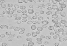
Figure 3.19. Image of a microbiological sample

Figure 3.19 comes from an acquisition system that is composed of an SM-6 optical microscope and a digital camera that can be operated with the help of a computer.

The optical level of the microscope and the resolution of the digital camera provide the link between the size of the image and the size of the sample (10 μm/48 pixels) to be studied.

The number of cells can be determined by bearing the following characteristics in mind:

– the cells have a round shape;

– the cells are of a similar size;

– the cells differ from the background in their color and intensity.

The process of determining the number of cells works as follows:

1. Application of a mask to adjust the color: white (W) for the cells and black (B) for the background.

2. Determining the fractal dimension and the fractal measurement (see definition 3.2) of the masked image comprising the interface of the background (K_WBW, d_WBW) as well as the interface of the cells (K_BW, d_BW) is done with the help of the following equations that are directly based on the definition of the fractal:

N_W and N_BW respectively represent the number of entirely white boxes as well as the number of partially black boxes.

d_BW and d_WBW are the fractal dimensions obtained with the help of the box-counting method (see section 3.2.3.1), K_BW and K_WBW are fractal measurements.

To determine the number of cells n_c as well as their radius r, the following equations are used:

From equations [3.2] and [3.3], the following equation is inferred:

s_m is the size of the box corresponding to the maximum fractal dimension. For a radius of r = 38 pixels, the fractal analysis estimates the number of cells which is equal to n_c= 100 cells. This is shown in Figure 3.20.

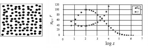
Figure 3.20. On the left: model of cellular structure, n_c = 100 cells of the radius r = 38 pixels. On the right: Determination of the number of cells n and their radius by fractal analysis (log s = 2 provides n_c = 100 and r = 38 pixels)

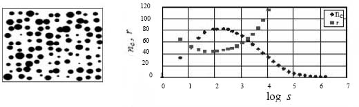
Figure 3.21. On the left: model of cellular structure n_c = 100 cells whose size is distributed according to a Gaussian law on the average radius r = 38 pixels of the standard deviation = 4. On the right: fractal analysis of the number of cells n and their radius r (log s = 2 provides nc = 82 and r = 43 pixels)

Note that unless the structures are of a certain size a bias is introduced in the estimation process (Figure 3.21), the number of cells that has been calculated is always lower than the number of cells in reality. The size of the cells is therefore underestimated.

Determining the number and the size of cells with the help of a fractal analysis is therefore only valid if the structures contain cells that are of a similar size.

This experiment shows that fractal analysis is a promising tool when it comes to counting and measuring objects in a digital image.

3.5.2. Using WTMM for the classification of textures – application in the field of medical imagery

Numerous works in image processing and pattern recognition are directed to two complex tasks: detection and automated classification of aggregates that might indicate the beginning of breast cancer.

This study, related to medical issues, is based on the application of the WTMM 2D method described in section 3.4.3. The aim of the segmentation of aggregates referred to as accumulation is to dip objects into the rough texture at a specific moment in time, shown in Figure 3.24.

As far as methodology is concerned, this technique is pertinent in discriminating against the groups of singularities that have been sufficiently characterized by the Hölder exponent.

Furthermore, the WTMM method is used to measure the properties of the invariance of the scale of mammography in order to distinguish dense tissue and adipose tissue with the help of the Hurst exponent.

In particular, the invariance of the observed scale is of a monofractal type in which two different groups of tissue are respectively characterized by the Hurst exponent H=0.3±0.05 and H=0.65±0.05. This type of result can be interpreted as an adipose feature of nature (fat) or as conjunctive (dense) tissue. The properties of invariance of a scale are associated with two groups of tissue that allow for the segmentation of the image of a breast. This procedure is based on the Hurst exponent of a square size of 256×256 pixels per analysis of around 50 images (see Figure 3.23).

This discrimination of monofractal behavior between adipose and dense tissue is also proven by the calculation of spectra for singularities D(h) (see Figure 3.22).

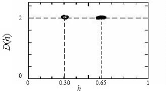
Figure 3.22. Spectrum of singularities of 49 juxtaposed images (512×512) on the level of scales 21≤ s ≤112

These spectra are made up of around 50 images and can be reduced to one single point h=H=0.30 for adipose tissue and h=H=0.65 for dense tissue. This is the proof that the texture represented in the mammogram is of a monofractal nature throughout the entire image. This is why it is possible to distinguish adipose from dense tissue.

For more information and more details on these concepts, please see Kestener’s thesis [KES 03].

Figure 3.23. Analysis based on WTMM of two mammograms: (a-d) breast with dense tissue and (e-h) breast with adipose tissue. The wavelet used in the analysis is an isotropic wavelet of the order 1 (derivate of a Gaussian function.) (a) and (e) represent the original mammogram; (b) and (f) represent their respective growth (zoom on the central part: 256×256 pixels); (c) and (g) show the WT modulus and the maxima chains at the level of s = 39 pixels; (d) and (h) show the chains of local maxima as well as their positions

Furthermore, this method is used to locate microcalcifications and characterize their disposition in a possible accumulation. In order to do this, the fractal dimension of all objects classed as “microcalcifications” are analyzed.

Figure 3.24. On the left: a mammogram showing microcalcifications. On the right: close-up on the area containing the cluster of microcalcifications

If the accumulation or cluster is of a linear disposition, the fractal dimension is equal to its Euclidean dimension d_f = 1, if a finite surface is filled d_f = 2 can be expected. However, if the cluster is of an arborescent structure, the fractal dimension is fractioned 1 < d_f < 2, which reflects the local complexity of mammary canals as well as the dissemination of the microcalcifications within these canals. An example of detecting microcalcifications in an accumulation or a cluster is shown in Figure 3.25. These images show that it is possible to clearly distinguish the areas of microcalcifications. Consequently, WTMM allows for an analysis and a characterization which still have to prove their effectiveness in clinical tests.

Figure 3.25. Detection of microcalcifications in a cluster (d_f = 2±0.05). (a) original mammogram. (b) and (c) Chains of maxima that indicate the microcalcifications for the scales s = 14 pixels and s = 24 pixels

In this study, the WTMM method confirms the interest in a fractal approach and shows that the Hölder exponent (or the Hurst exponent) can be used as an indicator of microcalcifications in the breast (probability of early stages of breast cancer) and, last but not least, this method also establishes the geometric shape of the cluster. This type of information could be used in combination with medical diagnosis and as an automatic system that helps medical staff with the diagnosis.

3.6. Conclusion

This chapter provides a pragmatic approach to the analysis of signals whose regularity varies from one point to another.

The concepts that have been used show multifractal analysis and wavelet analysis. In practice, the distribution of singularities is estimated by global measures using self-similarity or invariance on the scale of multifractals. The criterion of local regularity based on the Hölder exponent can be characterized as a decrease in the wavelet coefficients in the signal that is being analyzed. Furthermore, the spectrum of singularities of the multifractals to be studied is measured by local maxima of wavelet transform.

In the framework of this study, the formalism that was used has been validated in the field of health technology for the detection and characterization of images. Furthermore, the field of mechanical engineering looks at the process in terms of material fatigue.

This promising formalism is currently undergoing a fusion of ideas on its very basic level as well as in the area that aims at developing analysis tools.

3.7. Bibliography

[BEN 00] BENASSI A., COHEN S., DEGUY S., ISTAS J., “Self-similarity and intermittency”, in Wavelets and Time-frequency Signal Analysis, EPH, Cairo, Egypt, 2000.

[BER 94] BERAN J., Statistics for Long–Memory Process, Chapman and Hall, New York, 1994.

[BER 94] BERROIR J., Analyse multifractale d’images. Thesis, Paris University IX, 1994.

[BES 35] BESICOVITCH A.S., Mathematische Annalen 110, 1935.

[CAN 84] CANTOR G., “On the power of perfect sets of points”, Acta Mathematica 2, 1884.

[GRA 03] GRAZZINI J., Analyse multiéchelle et multifractale d’images météorologiques: application à la détection de zones précipitantes. Thesis, Marne-La-Vallée University, 2003.

[HAU 19] HAUSDORFF F., Mathematische Annalen 79, 157, 1919.

[JAF 91] JAFFARD S., “Pointwise smoothness, two-microlocalization and wavelet coefficients”, Publicaciones Matematiques, vol. 35, p. 155-168, 1991.

[KES 03] KESTENER P., Analyse multifractale 2D et 3D à l’aide de la transformation en ondelettes: application en mammographie et en turbulence développée. Thesis, Bordeaux University I, 2003.

[LEV 00] LEVY VEHEL J., “Analyse fractale: une nouvelle génération d’outils pour le traitement du signal-enjeux, tendances et évolution”, TSI 19 (1-2-3), pp. 335-350, 2000.

[LEV 97] LEVY VEHEL J., LUTTON E., TRICOT C., Fractal in Engineering. Springer Verlag, 1997.

[LEV 94] LEVY VEHEL J., MIGNOT P., “Multifractale segmentation of images”, Fractlas 2(3), pp. 371-377, 1994.

[LEV 92] LEVY VEHEL J., MIGNOT P., BERROIR J., “Multifractals, texture and image analysis”, In: Proc of Computer Vision and Pattern Recognition, CVPR’92, p. 661-664, 1992.

[MAN 82] MANDELBROT B.B., The Fractal Geometry of Nature, Freeman and Company, San Francisco, 1982.

[MAL 98] MALLAT F., A Wavelet Tour of Signal Processing, Academic Press, San Diego, 1998.

[OUA 02] OUAHABI A., LOPEZ A., BENDERBOUS S., “A wavelet-based method for compression, improving signal-to-noise and contrast in MR Images”, Proc. of the 2^nd. IEEE International Conference on Systems, Man & Cybernetics, Hammamet, Tunisia, 6-9 October 2002.

[SAM 94] SAMORODNITSKY G., TAQQU M.S., Stable Non-Gaussian Random Processes, Chapmann and Hall, 1994.

[VES 01] VESLA M., ZMESKAL O., VESELAY M., NEZADAL M., “Fractal analysis of image structures for microbiologic application”, HarFa, p. 9-10, 2001.

[VON 04] VON KOCH H., “Sur une courbe continue sans tangente, obtenue par une construction géometrique élémentaire”, Arkiv for Matematik 1, p. 681-704, 1904.