
In the previous chapter, you learned how to create and use Coherence caches without ever having to configure them explicitly. However, if you had paid close attention during the Coherence node startup, you might have noticed the log message that appears immediately after the banner that prints out the Coherence version, edition, and mode:
Oracle Coherence Version 3.5.1/461
Grid Edition: Development mode
Copyright (c) 2000, 2009, Oracle and/or its affiliates. All rights reserved.
Just like the default deployment descriptor, the default cache configuration file is packaged within coherence.jar, which is the reason why everything we've done so far has worked.
While this is great for trying things out quickly, it is not the optimal way to run Coherence in either the development or production environment, as you will probably want to have more control over things such as cache topology, data storage within the cache and its persistence outside of it, cache expiration, and so on.
Fortunately, Coherence is fully configurable and allows you to control all these things in detail. However, in order to make good decisions, you need to know when each of the various alternatives should be used.
That is the subject we will cover in this chapter. We will first discuss the different cache topologies and their respective strengths and weaknesses. We will then talk about various data storage strategies, which should provide you enough information to choose the one that best fits your needs. Finally, we will cover the Coherence cache configuration file and provide a sample configuration you can use as a starting point for your own applications.
So let's start by looking under the hood and learning more about the inner workings of Coherence.
You have already seen that using the Coherence cache is as simple as obtaining a reference to a NamedCache instance and using a Map-like API to get data from it (and put data into it). While the simplicity of the API is a great thing, it is important to understand what's going on under the hood so that you can configure Coherence in the most effective way, based on your application's data structures and data access patterns.
The simplicity of access to the Coherence named cache, from the API, might make you imagine the named cache as in the following diagram:
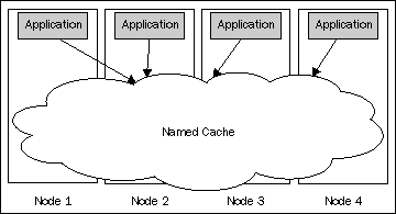
Basically, your application sees the Coherence named cache as a cloud-like structure that is spread across the cluster of nodes, but accessible locally using a very simple API. While this is a correct view from the client application's perspective, it does not fully reflect what goes on behind the scenes.
So let's clear the cloud and see what's hidden behind it.
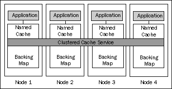
Whenever you invoke a method on a named cache instance, that method call gets delegated to the clustered cache service that the named cache belongs to. The preceding image depicts a single named cache managed by the single cache service, but the relationship between the named cache instances and the cache service is many to one—each named cache belongs to exactly one cache service, but a single cache service is typically responsible for more than one named cache.
The cache service is responsible for the distribution of cache data to appropriate members on cache writes, as well as for the retrieval of the data on cache reads.
However, the cache service is not responsible for the actual storage of the cached data. Instead, it delegates this responsibility to a backing map. There is one instance of the backing map 'per named cache per node', and this is where the cached data is actually stored.
There are many backing map implementations available out of the box, and we will discuss them shortly. For now, let's focus on the clustered cache services and the cache topologies they enable.
For each clustered cache you define in your application, you have to make an important choice—which cache topology to use.
There are two base cache topologies in Coherence: replicated and partitioned. They are implemented by two different clustered cache services, the Replicated Cache service and the Partitioned Cache service, respectively.
Note
Distributed or partitioned?
You will notice that the partitioned cache is often referred to as a distributed cache as well, especially in the API documentation and configuration elements.
This is somewhat of a misnomer, as both replicated and partitioned caches are distributed across many nodes, but unfortunately the API and configuration element names have to remain the way they are for compatibility reasons.
I will refer to them as partitioned throughout the book as that name better describes their purpose and functionality, but please remember this caveat when looking at the sample code and Coherence documentation that refers to distributed caches.
When the Coherence node starts and joins the cluster using the default configuration, it automatically starts both of these services, among others:
Services
(
TcpRing{...}
ClusterService{...}
InvocationService{Name=Management, ...}
Optimistic{Name=OptimisticCache, ...}
InvocationService{Name=InvocationService, ...}
)
While both replicated and partitioned caches look the same to the client code (remember, you use the same Map-based API to access both of them), they have very different performance, scalability, and throughput characteristics. These characteristics depend on many factors, such as the data set size, data access patterns, the number of cache nodes, and so on. It is important to take all of these factors into account when deciding the cache topology to use for a particular cache.
In the following sections, we will cover both cache topologies in more detail and provide some guidelines that will help you choose the appropriate one for your caches.
Note
Optimistic Cache service
You might also notice the Optimistic Cache service in the previous output, which is another cache service type that Coherence supports.
The Optimistic Cache service is very similar to the Replicated Cache service, except that it doesn't provide any concurrency control. It is rarely used in practice, so we will not discuss it separately.
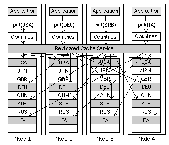
The most important characteristic of the replicated cache is that each cache item is replicated to all the nodes in the grid. That means that every node in the grid that is running the Replicated Cache service has the full dataset within a backing map for that cache.
For example, if we configure a Countries cache to use the Replicated Cache service and insert several objects into it, the data within the grid would look like the following:
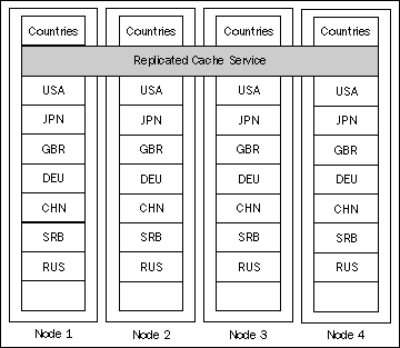
As you can see, the backing map for the Countries cache on each node has all the elements we have inserted.
This has significant implications on how and when you can use a replicated topology. In order to understand these implications better, we will analyze the replicated cache topology on four different criteria:
Read performance
Write performance
Data set size
Fault tolerance
Replicated caches have excellent, zero-latency read performance because all the data is local to each node, which means that an application running on that node can get data from the cache at in-memory speed.
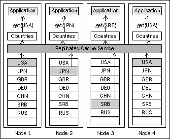
This makes replicated caches well suited for read-intensive applications, where minimal latency is required, and is the biggest reason you would consider using a replicated cache.
One important thing to note is that the locality of the data does not imply that the objects stored in a replicated cache are also in a ready-to-use, deserialized form. A replicated cache deserializes objects on demand. When you put the object into the cache, it will be serialized and sent to all the other nodes running the Replicated Cache service. The receiving nodes, however, will not deserialize the received object until it is requested, which means that you might incur a slight performance penalty when accessing an object in a replicated cache the first time. Once deserialized on any given node, the object will remain that way until an updated serialized version is received from another node.
In order to perform write operations, such as put, against the cache, the Replicated Cache service needs to distribute the operation to all the nodes in the cluster and receive confirmation from them that the operation was completed successfully. This increases both the amount of network traffic and the latency of write operations against the replicated cache. The write operation can be imagined from the following diagram:
To make things even worse, the performance of write operations against a replicated cache tends to degrade as the size of the cluster grows, as there are more nodes to synchronize.
All this makes a replicated cache poorly suited for write-intensive applications.
The fact that each node holds all the data implies that the total size of all replicated caches is limited by the amount of memory available to a single node. Of course, if the nodes within the cluster are not identical, this becomes even more restrictive and the limit becomes the amount of memory available to the smallest node in the cluster, which is why it is good practice to configure all the nodes in the cluster identically.
There are ways to increase the capacity of the replicated cache by using one of the backing map implementations that stores all or some of the cache data outside of the Java heap, but there is very little to be gained by doing so. As as soon as you move the replicated cache data out of RAM, you sacrifice one of the biggest advantages it provides: zero-latency read access.
This might not seem like a significant limitation considering that today's commodity servers can be equipped with up to 256 GB of RAM, and the amount will continue to increase in the future. (Come to think of it, this is 26 thousand times more than the first hard drive I had, and an unbelievable 5.6 million times more than 48 KB of RAM my good old ZX Spectrum had back in the eighties. It is definitely possible to store a lot of data in memory these days.)
However, there is a caveat—just because you can have that much memory in a single physical box, doesn't mean that you can configure a single Coherence node to use all of it. There is obviously some space that will be occupied by the OS, but the biggest limitation comes from today's JVMs and more specifically the way memory is managed within the JVM.
At the time of writing (mid 2009), there are hard limitations on how big your Coherence nodes can be; these are imposed by the underlying Java Virtual Machine (JVM).
The biggest problem is represented by the pauses that effectively freeze the JVM for a period of time during garbage collection. The length of this period is directly proportional to the size of the JVM heap, so, the bigger the heap, the longer it will take to reclaim the unused memory and the longer the node will seem frozen.
Once the heap grows over a certain size (2 GB at the moment for most JVMs), the garbage collection pause can become too long to be tolerated by users of an application, and possibly long enough that Coherence will assume the node is unavailable and kick it out of the cluster. There are ways to increase the amount of time Coherence waits for the node to respond before it kicks it out. However, it is usually not a good idea to do so as it might increase the actual cluster response time to the client application, even in the situations where the node really fails and should be removed from the cluster as soon as possible and its responsibilities transferred to another node.
Because of this, the recommended heap size for Coherence nodes is typically in the range of 1 to 2 GB, with 1 GB usually being the optimal size that ensures that garbage collection pauses are short enough to be unnoticeable. This severely limits the maximum size of the data set in a replicated cache.
Keeping the Coherence node size in a 1 to 2 GB range will also allow you to better utilize the processing power of your servers. As I mentioned earlier, Coherence can perform certain operations in parallel, across the nodes. In order to fully utilize modern servers, which typically have multiple CPUs, with two or four cores on each one, you will want to have multiple Coherence nodes on each physical server. There are no hard and fast rules here: you will have to test different configurations to determine which one works best for your application, but the bottom line is that in any scenario you will likely split your total available RAM across multiple nodes on a single physical box.
One of the new features introduced in Coherence 3.5 is the ability to manage data outside of the JVM heap, and I will cover it in more detail in the Backing maps section later in the chapter. Regardless, some information, such as indexes, is always stored on the JVM heap, so the heap size restriction applies to some extent to all configurations.
Replicated caches are very resilient to failure as there are essentially as many copies of the data as there are nodes in the cluster. When a single node fails, all that a Replicated Cache service needs to do in order to recover from the failure is to redirect read operations to other nodes and to simply ignore write operations sent to the failed node, as those same operations are simultaneously performed on the remaining cluster nodes.
When a failed node recovers or new node joins the cluster, failback is equally simple—the new node simply copies all the data from any other node in the cluster.
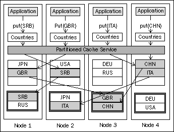
Unlike a replicated cache service, which simply replicates all the data to all cluster nodes, a partitioned cache service uses a divide and conquer approach—it partitions the data set across all the nodes in the cluster, as shown in the following diagram:
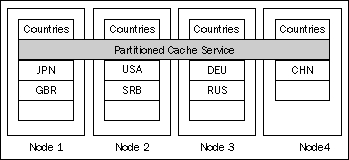
In this scenario, Coherence truly is reminiscent of a distributed hash map. Each node in the cluster becomes responsible for a subset of cache partitions (buckets), and the Partitioned Cache service uses an entry key to determine which partition (bucket) to store the cache entry in.
Let's evaluate the Partitioned Cache service using the same four criteria we used for the Replicated Cache service.
Because the data set is partitioned across the nodes, it is very likely that the reads coming from any single node will require an additional network call. As a matter of fact, we can easily prove that in a general case, for a cluster of N nodes, (N-1)/N operations will require a network call to another node.
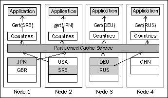
This is depicted in the preceding diagram, where three out of the four requests were processed by a node different from the one issuing the request.
However, it is important to note that if the requested piece of data is not managed locally, it will always take only one additional network call to get it, because the Partitioned Cache service is able to determine which node owns a piece of data based on the requested key. This allows Coherence to scale extremely well in a switched network environment, as it utilizes direct point-to-point communication between the nodes.
Another thing to consider is that the objects in a partitioned cache are always stored in a serialized binary form. This means that every read request will have to deserialize the object, introducing additional latency.
The fact that there is always at most one network call to retrieve the data ensures that reads from a partitioned cache execute in constant time. However, because of that additional network call and deserialization, this is still an order of magnitude slower than a read from a replicated cache.
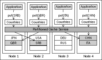
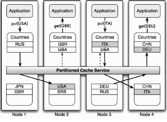
In the simplest case, partitioned cache write performance is pretty much the same as its read performance. Write operations will also require network access in the vast majority of cases, and they will use point-to-point communication to accomplish the goal in a single network call, as shown in the following screenshot
However, this is not the whole story, which is why I said "in the simplest case".
One thing you are probably asking yourself by now is "but what happens if a node fails?". Rest assured, partitioned caches can be fully fault tolerant, and we will get into the details of that in a section on fault tolerance. For now, let's fix the preceding diagram to show what partitioned cache writes usually look like.
As you can see from the diagram, in addition to the backing map that holds the live cache data, the partitioned cache service also manages another map on each node—a backup storage.
Backup storage is used to store backup copies of cache entries, in order to ensure that no data is lost in the case of a node failure. Coherence ensures that backup copies of primary entries from a particular node are stored not only on a different node, but also on a different physical server if possible. This is necessary in order to ensure that data is safe even in the case of hardware failure, in which case all the nodes on that physical machine would fail simultaneously.
You can configure the number of backup copies Coherence should create. The default setting of one backup copy, as the preceding diagram shows, is the most frequently used configuration. However, if the objects can be easily restored from a persistent data store, you might choose to set the number of backup copies to zero, which will have a positive impact on the overall memory usage and the number of objects that can be stored in the cluster.
You can also increase the number of backup copies to more than one, but this is not recommended by Oracle and is rarely done in practice. The reason for this is that it guards against a very unlikely scenario—that two or more physical machines will fail at exactly the same time.
The chances are that you will either lose a single physical machine, in the case of hardware failure, or a whole cluster within a data center, in the case of catastrophic failure. A single backup copy, on a different physical box, is all you need in the former case, while in the latter no number of backup copies will be enough—you will need to implement much broader disaster recovery solution and guard against it by implementing cluster-to-cluster replication across multiple data centers.
If you use backups, that means that each partitioned cache write will actually require at least two network calls: one to write the object into the backing map of the primary storage node and one or more to write it into the backup storage of each backup node.
This makes partitioned cache writes somewhat slower than reads, but they still execute in constant time and are significantly faster than replicated cache writes.
Because each node stores only a small (1/N) portion of the data set, the size of the data set is limited only by the total amount of space that is available to all the nodes in the cluster. This allows you to manage very large data sets in memory, and to scale the cluster to handle growing data sets by simply adding more nodes. Support for very large in-memory data sets (potentially terabytes in Coherence 3.5) is one of the biggest advantages of a partitioned over a replicated cache, and is often the main reason to choose it.
That said, it is important to realize that the actual amount of data you can store is significantly lower than the total amount of RAM in the cluster. Some of the reasons for this are obvious—if your data set is 1 GB and you have one backup copy for each object, you need at least 2 GB of RAM. However, there is more to it than that.
For one, your operating system and Java runtime will use some memory. How much exactly varies widely across operating systems and JVM implementations, but it won't be zero in any case. Second, the cache indexes you create will need some memory. Depending on the number of indexes and the size of the indexed properties and corresponding cache keys, this might amount to a significant quantity. Finally, you need to leave enough free space for execution of both Coherence code and your own code within each JVM, or a frequent full garbage collection will likely bring everything to a standstill, or worse yet, you will run out of memory and most likely bring the whole cluster down—when one node fails in a low-memory situation, it will likely have a domino effect on other nodes as they try to accommodate more data than they can handle.
Because of this, it is important that you size the cluster properly and use cache expiration and eviction policies to control the amount of data in the cache.
As we discussed in the section on write performance, a Partitioned Cache service allows you to keep one or more backups of cache data in order to prevent data loss in the case of a node failure.
When a node fails, the Partitioned Cache service will notify all other nodes to promote backup copies of the data that the failed node had primary responsibility for, and to create new backup copies on different nodes.
When the failed node recovers, or a new node joins the cluster, the Partitioned Cache service will fail back some of the data to it by repartitioning the cluster and asking all of the existing members to move some of their data to the new node.
It should be obvious by now that the partitioned cache should be your topology of choice for large, growing data sets, and write-intensive applications.
However, as I mentioned earlier, there are several Coherence features that are built on top of partitioned cache that make it preferable for many read-intensive applications as well. We will discuss one of these features in detail next and briefly touch upon the second one, which will be covered in a lot more detail later in the book.
A near cache is a hybrid, two-tier caching topology that uses a combination of a local, size-limited cache in the front tier, and a partitioned cache in the back tier to achieve the best of both worlds: the zero-latency read access of a replicated cache and the linear scalability of a partitioned cache.
Basically, the near cache is a named cache implementation that caches a subset of the data locally and responds to read requests for the data within that subset directly, without asking the Partitioned Cache service to handle the request. This eliminates both network access and serialization overhead associated with the partitioned cache topology, and allows applications to obtain data objects at the same speed as with replicated caches.
On the other hand, the near cache simply delegates cache writes to the partitioned cache behind it, so the write performance is almost as good as with the partitioned cache (there is some extra overhead to invalidate entries in the front cache).
One problem typically associated with locally cached data is that it could become stale as the master data in the backend store changes. For example, if a near cache on a node A has object X cached locally, and node B updates object X in the cluster, the application running on node A (and other nodes that have object X cached locally) might end up holding a stale, and potentially incorrect, version of object X...
Fortunately, Coherence provides several invalidation strategies that allow the front tier of a near cache to evict stale objects based on the changes to the master copy of those objects, in a back-tier partitioned cache.
This strategy, as its name says, doesn't actually do anything to evict stale data.
The reason for that is that for some applications it doesn't really matter if the data is somewhat out of date. For example, you might have an e-commerce website that displays the current quantity in stock for each product in a catalog. It is usually not critical that this number is always completely correct—a certain degree of staleness is OK.
However, you probably don't want to keep using the stale data forever. So, you need to configure the front-tier cache to use time-based expiration with this strategy, based on how current your data needs to be.
The main benefit of the None strategy is that it scales extremely well, as there is no extra overhead that is necessary to keep the data in sync, so you should seriously consider it if your application can allow some degree of data staleness.
The Present strategy uses event listeners to evict the front cache data automatically when the data in a back-tier cache changes.
It does that by registering a key-based listener for each entry that is present in its front cache (thus the name). As soon as one of those entries changes in a back cache or gets deleted, the near cache receives an event notification and evicts the entry from its front cache. This ensures that the next time an application requests that particular entry, the latest copy is retrieved from the back cache and cached locally until the next invalidation event is received.
This strategy has some overhead, as it registers as many event listeners with the partitioned cache as there are items in the front cache. This requires both processing cycles within the cluster to determine if an event should be sent, and network access for the listener registration and deregistration, as well as for the event notifications themselves.
One thing to keep in mind is that the invalidation events are sent asynchronously, which means that there is still a time window (albeit very small, typically in the low milliseconds range) during which the value in the front cache might be stale. This is usually acceptable, but if you need to ensure that the value read is absolutely current, you can achieve that by locking it explicitly before the read. That will require a network call to lock the entry in the back cache, but it will ensure that you read the latest version.
Just like the Present strategy, the All strategy uses Coherence events to keep the front cache from becoming stale. However, unlike the Present strategy, which registers one listener for each cache entry, the All strategy registers only a single listener with a back cache, but that single listener listens to all the events.
There is an obvious trade-off here: registering many listeners with the back cache, as the Present strategy does, will require more CPU cycles in the cluster to determine whether an event notification should be sent to a particular near cache, but every event received by the near cache will be useful. On the other hand, using a single listener to listen for all cache events, as the All strategy does, will require less cycles to determine if an event notification should be sent, but will result in a lot more notifications going to a near cache, usually over the network. Also, the near cache will then have to evaluate them and decide whether it should do anything about them or not, which requires more CPU cycles on a node running the near cache than the simple eviction as a result of an event notification for a Present strategy.
The choice of Present or All depends very much on the data access pattern. If the data is mostly read and typically updated by the node that has it cached locally (as is the case with session state data when sticky load balancing is used, for example), the Present strategy tends to work better. However, if the updates are frequent and there are many near caches with a high degree of overlap in their front caches, you will likely get better results using the All strategy, as many of the notifications will indeed be applicable to all of them.
That said, the best way to choose the strategy is to run some realistic performance tests using both and to see how they stack up.
The final invalidation strategy is the Auto strategy, which according to the documentation "switches between Present and All based on the cache statistics". Unfortunately, while that might have been the goal, the current implementation simply defaults to All, and there are indications that it might change in the future to default to Present instead.
This wouldn't be too bad on its own, but the problem is that Auto is also the default strategy for near cache invalidation. That means that if its implementation does indeed change in the future, all of the near caches using default invalidation strategy will be affected.
Because of this, you should always specify the invalidation strategy when configuring a near cache. You should choose between Present and All if event-based invalidation is required, or use None if it isn't.
The near cache allows you to achieve the read performance of a replicated cache as well as the write performance and scalability of a partitioned cache. This makes it the best topology choice for the read-mostly or balanced read-write caches that need to support data sets of any size.
This description will likely fit many of the most important caches within your application, so you should expect to use near cache topology quite a bit.
The Continuous Query Cache (CQC) is conceptually very similar to a near cache. For one, it also has a zero-latency front cache that holds a subset of the data, and a slower but larger back cache, typically a partitioned cache, that holds all the data. Second, just like the near cache, it registers a listener with a back cache and updates its front cache based on the event notifications it receives.
However, there are several major differences as well:
CQC populates its front cache based on a query as soon as it is created, unlike the near cache, which only caches items after they have been requested by the application.
CQC registers a query-based listener with a back cache, which means that its contents changes dynamically as the data in the back cache changes. For example, if you create a CQC based on a Coherence query that shows all open trade orders, as the trade orders are processed and their status changes they will automatically disappear from a CQC. Similarly, any new orders that are inserted into the back cache with a status set to
Openwill automatically appear in the CQC. Basically, CQC allows you to have a live dynamic view of the filtered subset of data in a partitioned cache.CQC can only be created programmatically, using the Coherence API. It cannot be configured within a cache configuration descriptor.
Because of the last point, we will postpone the detailed discussion on the CQC until we cover both cache events and queries in more detail, but keep in mind that it can be used to achieve a similar result to that which a near cache allows you to achieve via configuration: bringing a subset of the data closer to the application, in order to allow extremely fast, zero-latency read access to it without sacrificing write performance.
It is also an excellent replacement for a replicated cache—by simply specifying a query that returns all objects, you can bring the whole data set from a back cache into the application's process, which will allow you to access it at in-memory speed.
Now that we have covered various cache topologies, it is time to complete the puzzle by learning more about backing maps.
As you learned earlier, the backing map is where cache data within the cluster is actually stored, so it is a very important piece within the Coherence architecture. So far we have assumed that a backing map stores all the data in memory, which will be the case for many applications as it provides by far the best performance. However, there are situations where storing all the data in memory is either impossible, because the data set is simply too big, or impractical, because a large part of the data is rarely accessed and there is no need to have the fastest possible access to it at all times.
One of the nicest things about Coherence is that it is extremely flexible and configurable. You can combine different pieces that are available out of the box, such as caching services and backing maps, in many different ways to solve many difficult distributed data management problems. If nothing fits the bill, you can also write your own, custom implementations of various components, including backing maps.
However, there is rarely a need to do so, as Coherence ships with a number of useful backing map implementations that can be used to store data both on-heap as well as off-heap. We will discuss all of them in the following sections so you can make an informed decision when configuring backing maps for your caches.
The local cache is commonly used both as the backing map for replicated and partitioned caches and as a front cache for near and continuous query caches. It stores all the data on the heap, which means that it provides by far the fastest access speed, both read and write, compared to other backing map implementations.
The local cache can be size-limited to a specific number of entries, and will automatically prune itself when the limit is reached, based on the specified eviction policy: LRU (Least Recently Used), LFU (Least Frequently Used), or HYBRID, which is the default and uses a combination of LRU and LFU to determine which items to evict. Of course, if none of these built-in eviction policies works for you, Coherence allows you to implement and use a custom one.
You can also configure the local cache to expire cache items based on their age, which is especially useful when it is used as a front cache for a near cache with invalidation strategy set to none.
Finally, the local cache implements full Map, CacheMap, and ObservableMap APIs, which means that you can use it within your application as a more powerful HashMap, which in addition to the standard Map operations supports item expiration and event notifications, while providing fully thread-safe, highly concurrent access to its contents.
The external backing map allows you to store cache items off-heap, thus allowing far greater storage capacity, at the cost of somewhat-to-significantly worse performance.
There are several pluggable storage strategies that you can use with an external backing map, which allow you to configure where and how the data will be stored. These strategies are implemented as storage managers:
NIO Memory Manager: This uses an off-heap NIO buffer for storage. This means that it is not affected by the garbage collection times, which makes it a good choice for situations where you want to have fast access to data, but don't want to increase the size or the number of Coherence JVMs on the server.
NIO File Manager: This uses NIO memory-mapped files for data storage. This option is generally not recommended as its performance can vary widely depending on the OS and JVM used. If you plan to use it, make sure that you run some performance tests to make sure it will work well in your environment.
Berkeley DB Store Manager: This uses Berkeley DB Java Edition embedded database to implement on-disk storage of cache items.
In addition to these concrete storage manager implementations, Coherence ships with a wrapper storage manager that allows you to make write operations asynchronous for any of the store managers listed earlier. You can also create and use your own custom storage manager by creating a class that implements the com.tangosol.io.BinaryStoreManager interface.
Just like the local cache, the external backing map can be size limited and can be configured to expire cache items based on their age. However, keep in mind that the eviction of cache items from disk-based caches can be very expensive. If you need to use it, you should seriously consider using the paged external backing map instead.
The paged external backing map is very similar to the external backing map described previously. They both support the same set of storage managers, so your storage options are exactly the same. The big difference between the two is that a paged external backing map uses paging to optimize LRU eviction.
Basically, instead of storing cache items in a single large file, a paged backing map breaks it up into a series of pages. Each page is a separate store, created by the specified store manager. The page that was last created is considered current and all write operations are performed against that page until a new one is created.
You can configure both how many pages of data should be stored and the amount of time between page creations. The combination of these two parameters determines how long the data is going to be kept in the cache. For example, if you wanted to cache data for an hour, you could configure the paged backing map to use six pages and to create a new page every ten minutes, or to use four pages with new one being created every fifteen minutes.
Once the page count limit is reached, the items in the oldest page are considered expired and are evicted from the cache, one page at a time. This is significantly more efficient than the individual delete operations against the disk-based cache, as in the case of a regular external backing map.
The overflow backing map is a composite backing map with two tiers: a fast, size-limited, in-memory front tier, and a slower, but potentially much larger back tier on a disk. At first sight, this seems to be a perfect way to improve read performance for the most recently used data while allowing you to store much larger data sets than could possibly fit in memory.
However, using an overflow backing map in such a way is not recommended. The problem is that the access to a disk-based back tier is much slower than the access to in-memory data. While this might not be significant when accessing individual items, it can have a huge negative impact on operations that work with large chunks of data, such as cluster repartitioning.
A Coherence cluster can be sized dynamically, by simply adding nodes or removing nodes from it. The whole process is completely transparent and it does not require any changes in configuration—you simply start new nodes or shut down existing ones. Coherence will automatically rebalance the cluster to ensure that each node handles approximately the same amount of data.
When that happens, whole partitions need to be moved from one node to another, which can be quite slow when disk-based caches are used, as is almost always the case with the overflow backing map. During the repartitioning requests targeted to partitions that are being moved are blocked, and the whole cluster might seem a bit sluggish, or in the worst case scenario completely stalled, so it is important to keep repartitioning as short as possible.
Because of this, it is recommended that you use an overflow map only when you are certain that most of the data will always fit in memory, but need to guard against occasional situations where some data might need to be moved to disk because of a temporary memory shortage. Basically, the overflow backing map can be used as a substitute for an eviction policy in these situations.
If, on the other hand, you need to support much larger data sets than could possibly fit in memory, you should use a read-write backing map instead.
The read-write backing map is another composite backing map implementation. However, unlike the overflow backing map, which has a two-tiered cache structure, the read-write backing map has a single internal cache (usually a local cache) and either a cache loader, which allows it to load data from the external data source on cache misses, or a cache store, which also provides the ability to update data in the external data store on cache puts.
As such, the read-write backing map is a key enabler of the read-through/ write-through architecture that places Coherence as an intermediate layer between the application and the data store, and allows for a complete decoupling between the two. It is also a great solution for situations where not all the data fits in memory, as it does not have the same limitations as overflow backing map does.
The key to making a read-write backing map work is to use it in front of a shared data store that can be accessed from all the nodes. The most obvious and commonly used data source that fits that description is a relational database, so Coherence provides several cache loader and cache store implementations for relational database access out of the box, such as JPA, Oracle TopLink, and Hibernate.
However, a read-write backing map is not limited to a relational database as a backend by any means. It can also be used in front of web services, mainframe applications, a clustered file system, or any other shared data source that can be accessed from Java.
By default, a single backing map is used to store the entries from all cache partitions on a single node. This imposes certain restrictions on how much data each node can store.
For example, if you choose to use local cache as a backing map, the size of the backing map on a single node will be limited by the node's heap size. In most cases, this configuration will allow you to store up to 300-500 MB per node, because of the heap size limitations discussed earlier.
However, even if you decide to use NIO buffer for off-heap storage, you will be limited by the maximum direct buffer size Java can allocate, which is 2 GB (as a 32-bit integer is used to specify the size of the buffer). While you can still scale the size of the cache by adding more nodes, there is a practical limit to how far you can go. The number of CPUs on each physical machine will determine the upper limit for the number on nodes you can run, so you will likely need 100 or more physical boxes and 500 Coherence nodes in order to store 1 TB of data in a single cache.
In order to solve this problem and support in-memory caches in the terabytes range without increasing the node count unnecessarily, the partitioned backing map was introduced in Coherence 3.5.
The partitioned backing map contains one backing map instance for each cache partition, which allows you to scale the cache size by simply increasing the number of partitions for a given cache. Even though the theoretical limit is now 2 GB per partition, you have to keep in mind that a partition is a unit of transfer during cache rebalancing, so you will want to keep it significantly smaller (the officially recommended size for a single partition is 50 MB).
That means that you need to divide the expected cache size by 50 MB to determine the number of partitions. For example, if you need to store 1 TB of data in the cache, you will need at least 20,972 partitions. However, because the number of partitions should always be a prime number, you should set it to the next higher prime number, which in this case is 20,981 (you can find the list of first 10,000 prime numbers, from 1 to 104,729, at http://primes.utm.edu/lists/small/10000.txt).
The important thing to keep in mind is that the number of partitions has nothing to do with the number of nodes in the cluster—you can spread these 20 thousand plus partitions across 10 or 100 nodes, and 5 or 50 physical machines. You can even put them all on a single box, which will likely be the case during testing.
By making cache size dependent solely on the number of partitions, you can fully utilize the available RAM on each physical box and reach 1 TB cache size with a significantly smaller number of physical machines and Coherence nodes. For example, 50 nodes, running on 10 physical machines with 128 GB of RAM each, could easily provide you with 1 TB of in-memory storage.
Note
Partitioned backing map and garbage collection
I mentioned earlier that you need to keep heap size for each Coherence JVM in the 1-2 GB range, in order to avoid long GC pauses.
However, this is typically not an issue with a partitioned backing map, because it is usually used in combination with off-heap, NIO buffer-based storage.
Now that you understand the available cache topologies and data storage options, let's return to the subject we started this chapter with.
What you will realize when you start identifying entities within your application and planning caches for them is that many of those entities have similar data access patterns. Some will fall into the read-only or read-mostly category, such as reference, and you can decide to use either a replicated cache or a partitioned cache fronted by a near or continuous query cache for them.
Others will fall into a transactional data category, which will tend to grow in size over time and will have a mixture of reads and writes. These will typically be some of the most important entities that the application manages, such as invoices, orders, and customers. You will use partitioned caches to manage those entities, possibly fronted with a near cache depending on the ratio of reads to writes.
You might also have some write-mostly data, such as audit trail or log entries, but the point is that in the end, when you finish analyzing your application's data model, you will likely end up with a handful of entity categories, even though you might have many entity types.
If you had to configure a cache for each of these entity types separately, you would end up with a lot of repeated configuration, which would be very cumbersome to maintain if you needed to change something for each entity that belongs to a particular category.
This is why the Coherence cache configuration has two parts: caching schemes and cache mappings. The former allows you to define a single configuration template for all entities in a particular category, while the latter enables you to map specific named caches to a particular caching scheme.
Caching schemes are used to define cache topology, as well as other cache configuration parameters, such as which backing map to use, how to limit cache size and expire cache items, where to store backup copies of the data, and in the case of a read-write backing map, even how to load data into the cache from the persistent store and how to write it back into the store.
While there are only a few top-level caching schemes you are likely to use, which pretty much map directly to the cache topologies we discussed in the first part of this chapter, there are many possible ways to configure them. Covering all possible configurations would easily fill a book on its own, so we will not go that far. In the remainder of this chapter we will look at configuration examples for the commonly used cache schemes, but even for those I will not describe every possible configuration option.
The Coherence Developer's Guide is your best resource on various options available for cache configuration using any of the available schemes, and you should now have enough background information to understand various configuration options available for each of them. I strongly encourage you to review the Appendix D: Cache Configuration Elements section in the Developer's Guide for more information about all configuration parameters for a particular cache topology and backing map you are interested in.
Let's look at an example of a caching scheme definition under a microscope, to get a better understanding of what it is made of.
<distributed-scheme>
<scheme-name>example-distributed</scheme-name>
<service-name>DistributedCache</service-name>
<backing-map-scheme>
<local-scheme>
<scheme-ref>example-binary-backing-map</scheme-ref>
</local-scheme>
</backing-map-scheme>
<autostart>true</autostart>
</distributed-scheme>
The preceding code is taken directly from the sample cache configuration file that is shiped with Coherence, and you have seen it before, when you issued the cache countries command in the Coherence Console in the previous chapter.
The top-level element, distributed-scheme, tells us that any cache that uses this scheme will use a partitioned topology (this is one of those unfortunate instances where distributed is used instead of partitioned for backwards compatibility reasons).
The scheme-name element allows us to specify a name for the caching scheme, which we can later use within cache mappings and when referencing a caching scheme from another caching scheme, as we'll do shortly.
The service-name element is used to specify the name of the cache service that all caches using this particular scheme will belong to. While the service type is determined by the root element of the scheme definition, the service name can be any name that is meaningful to you. However, there are two things you should keep in mind when choosing a service name for a scheme:
Coherence provides a way to ensure that the related objects from different caches are stored on the same node, which can be very beneficial from a performance standpoint. For example, you might want to ensure that the account and all transactions for that account are collocated. You will learn how to do that in the next chapter, but for now you should remember that this feature requires that all related caches belong to the same cache service. This will automatically be the case for all caches that are mapped to the same cache scheme, but in the cases when you have different schemes defined for related caches, you will need to ensure that service name for both schemes is the same.
All caches that belong to the same cache service share a pool of threads. In order to avoid deadlocks, Coherence prohibits re-entrant calls from the code executing on a cache service thread into the same cache service. One way to work around this is to use separate cache services. For example, you might want to use separate services for reference and transactional caches, which will allow you to access reference data without any restrictions from the code executing on a service thread of a transactional cache.
The next element, backing-map-scheme, defines the type of the backing map we want all caches mapped to this caching scheme to use. In this example, we are telling Coherence to use local cache as a backing map. Note that while many named caches can be mapped to this particular caching scheme, each of them will have its own instance of the local cache as a backing map. The configuration simply tells the associated cache service which scheme to use as a template when creating a backing map instance for the cache.
The scheme-ref element within the local-scheme tells us that the configuration for the backing map should be loaded from another caching scheme definition, example-binary-backing-map. This is a very useful feature, as it allows you to compose new schemes from the existing ones, without having to repeat yourself.
Finally, the autostart element determines if the cache service for the scheme will be started automatically when the node starts. If it is omitted or set to false, the service will start the first time any cache that belongs to it is accessed. Normally, you will want all the services on your cache servers to start automatically.
The scheme definition shown earlier references the local cache scheme named example-binary-backing-scheme as its backing map. Let's see what the referenced definition looks like:
<local-scheme>
<scheme-name>example-binary-backing-map</scheme-name>
<eviction-policy>HYBRID</eviction-policy>
<high-units>{back-size-limit 0}</high-units>
<unit-calculator>BINARY</unit-calculator>
<expiry-delay>{back-expiry 1h}</expiry-delay>
<flush-delay>1m</flush-delay>
<cachestore-scheme></cachestore-scheme>
</local-scheme>
You can see that the local-scheme allows you to configure various options for the local cache, such as eviction policy, the maximum number of units to keep within the cache, as well as expiry and flush delay.
The high-units and unit-calculator elements are used together to limit the size of the cache, as the meaning of the former is defined by the value of the latter. Coherence uses unit calculator to determine the "size" of cache entries. There are two built-in unit calculators: fixed and binary.
The difference between the two is that the first one simply treats each cache entry as a single unit, allowing you to limit the number of objects in the cache, while the second one uses the size of a cache entry (in bytes) to represent the number of units it consumes. While the latter gives you much better control over the memory consumption of each cache, its use is constrained by the fact that the entries need to be in a serialized binary format, which means that it can only be used to limit the size of a partitioned cache.
In other cases you will either have to use the fixed calculator to limit the number of objects in the cache, or write your own implementation that can determine the appropriate unit count for your objects (if you decide to write a calculator that attempts to determine the size of deserialized objects on heap, you might want to consider using com.tangosol.net.cache.SimpleMemoryCalculator as a starting point).
One important thing to note in the example on the previous page is the use of macro parameters to define the size limit and expiration for the cache, such as {back-size-limit 0} and {back-expiry 1h}. The first value within the curly braces is the name of the macro parameter to use, while the second value is the default value that should be used if the parameter with the specified name is not defined. You will see how macro parameters and their values are defined shortly, when we discuss cache mappings.
Near cache is a composite cache, and requires us to define separate schemes for the front and back tier. We could reuse both scheme definitions we have seen so far to create a definition for a near cache:
<near-scheme>
<scheme-name>example-near</scheme-name>
<front-scheme>
<local-scheme>
<scheme-ref>example-binary-backing-map</scheme-ref>
</local-scheme>
</front-scheme>
<back-scheme>
<distributed-scheme>
<scheme-ref>example-distributed</scheme-ref>
</distributed-scheme>
</back-scheme>
<invalidation-strategy>present</invalidation-strategy>
<autostart>true</autostart>
</near-scheme>
Unfortunately, the example-binary-backing-map won't quite work as a front cache in the preceding definition—it uses the binary unit calculator, which cannot be used in the front tier of a near cache. In order to solve the problem, we can override the settings from the referenced scheme:
<front-scheme>
<local-scheme>
<scheme-ref>example-binary-backing-map</scheme-ref>
</local-scheme>
</front-scheme>
However, in this case it would probably make more sense not to use reference for the front scheme definition at all, or to create and reference a separate local scheme for the front cache.
Using local cache as a backing map is very convenient during development and testing, but more likely than not you will want your data to be persisted as well. If that's the case, you can configure a read-write backing map as a backing map for your distributed cache:
<distributed-scheme>
<scheme-name>example-distributed</scheme-name>
<service-name>DistributedCache</service-name>
<backing-map-scheme>
<read-write-backing-map-scheme>
<internal-cache-scheme>
<local-scheme/>
</internal-cache-scheme>
<cachestore-scheme>
<class-scheme>
<class-name>
com.tangosol.coherence.jpa.JpaCacheStore
</class-name>
<init-params>
<init-param>
<param-type>java.lang.String</param-type>
<param-value>{cache-name}</param-value>
</init-param>
<init-param>
<param-type>java.lang.String</param-type>
<param-value>{class-name}</param-value>
</init-param>
<init-param>
<param-type>java.lang.String</param-type>
<param-value>PersistenceUnit</param-value>
</init-param>
</init-params>
</class-scheme>
</cachestore-scheme>
</read-write-backing-map-scheme>
</backing-map-scheme>
<autostart>true</autostart>
</distributed-scheme>
The read-write backing map defined previously uses unlimited local cache to store the data, and a JPA-compliant cache store implementation that will be used to persist the data on cache puts, and to retrieve it from the database on cache misses.
We will discuss JPA cache store in much more detail in Chapter 8, Implementing the Persistence Layer, but from the preceding example it should be fairly obvious that its constructor accepts three arguments: entity name, which is in this example equivalent to a cache name, fully qualified name of entity class, and the name of the JPA persistence unit defined in the persistence.xml file.
As we discussed earlier, the partitioned backing map is your best option for very large caches. The following example demonstrates how you could configure a partitioned backing map that will allow you to store 1 TB of data in a 50-node cluster, as we discussed earlier:
<distributed-scheme>
<scheme-name>large-scheme</scheme-name>
<service-name>LargeCacheService</service-name>
<partition-count>20981</partition-count>
<backing-map-scheme>
<partitioned>true</partitioned>
<external-scheme>
<high-units>20</high-units>
<unit-calculator>BINARY</unit-calculator>
<unit-factor>1073741824</unit-factor>
<nio-memory-manager>
<initial-size>1MB</initial-size>
<maximum-size>50MB</maximum-size>
</nio-memory-manager>
</external-scheme>
</backing-map-scheme>
<backup-storage>
<type>off-heap</type>
<initial-size>1MB</initial-size>
<maximum-size>50MB</maximum-size>
</backup-storage>
<autostart>true</autostart>
</distributed-scheme>
We have configured partition-count to 20,981, which will allow us to store 1 TB of data in the cache while keeping the partition size down to 50 MB.
We have then used the partitioned element within the backing map scheme definition to let Coherence know that it should use the partitioned backing map implementation instead of the default one.
The external-scheme element is used to configure the maximum size of the backing map as a whole, as well as the storage for each partition. Each partition uses an NIO buffer with the initial size of 1 MB and a maximum size of 50 MB.
The backing map as a whole is limited to 20 GB using a combination of high-units, unit-calculator, and unit-factor values. Because we are storing serialized objects off-heap, we can use binary calculator to limit cache size in bytes. However, the high-units setting is internally represented by a 32-bit integer, so the highest value we could specify for it would be 2 GB.
In order allow for larger cache sizes while preserving backwards compatibility, Coherence engineers decided not to widen high-units to 64 bits. Instead, they introduced the unit-factor setting, which is nothing more than a multiplier for the high-units value. In the preceding example, the unit-factor is set to 1 GB, which in combination with the high-units setting of 20 limits cache size per node to 20 GB.
Finally, when using a partitioned backing map to support very large caches off-heap, we cannot use the default, on-heap backup storage. The backup storage is always managed per partition, so we had to configure it to use off-heap buffers of the same size as primary storage buffers.
Finally, we can use a partitioned read-write backing map to support automatic persistence for very large caches. The following example is really just a combination of the previous two examples, so I will not discuss the details. It is also a good illustration of the flexibility Coherence provides when it comes to cache configuration.
<distributed-scheme>
<scheme-name>large-persistent-scheme</scheme-name>
<service-name>LargePersistentCacheService</service-name>
<partition-count>20981</partition-count>
<backing-map-scheme>
<partitioned>true</partitioned>
<read-write-backing-map-scheme>
<internal-cache-scheme>
<external-scheme>
<high-units>20</high-units>
<unit-calculator>BINARY</unit-calculator>
<unit-factor>1073741824</unit-factor>
<nio-memory-manager>
<initial-size>1MB</initial-size>
<maximum-size>50MB</maximum-size>
</nio-memory-manager>
</external-scheme>
</internal-cache-scheme>
<cachestore-scheme>
<class-scheme>
<class-name>
com.tangosol.coherence.jpa.JpaCacheStore
</class-name>
<init-params>
<init-param>
<param-type>java.lang.String</param-type>
<param-value>{cache-name}</param-value>
</init-param>
<init-param>
<param-type>java.lang.String</param-type>
<param-value>{class-name}</param-value>
</init-param>
<init-param>
<param-type>java.lang.String</param-type>
<param-value>SigfePOC</param-value>
</init-param>
</init-params>
</class-scheme>
</cachestore-scheme>
</read-write-backing-map-scheme>
</backing-map-scheme>
<backup-storage>
<type>off-heap</type>
<initial-size>1MB</initial-size>
<maximum-size>50MB</maximum-size>
</backup-storage>
<autostart>true</autostart>
</distributed-scheme>
This concludes our discussion of caching schemes—it is now time to see how we can map our named caches to them.
Cache mappings allow you to map cache names to the appropriate caching schemes:
<cache-mapping>
<cache-name>repl-*</cache-name>
<scheme-name>example-replicated</scheme-name>
</cache-mapping>
You can map either a full cache name, or a name pattern, as in the previous example. What this definition is basically saying is that whenever you call the CacheFactory.getCache method with a cache name that starts with repl-, a caching scheme with the name example-replicated will be used to configure the cache.
Coherence will evaluate cache mappings in order, and will map the cache name using the first pattern that matches. That means that you need to specify cache mappings from the most specific to the least specific.
Cache mappings can also be used to specify macro parameters used within a caching scheme definition:
<cache-mapping>
<cache-name>near-accounts</cache-name>
<scheme-name>example-near</scheme-name>
<init-params>
<init-param>
</init-param>
</init-params>
</cache-mapping>
<cache-mapping>
<cache-name>dist-*</cache-name>
<scheme-name>example-distributed</scheme-name>
<init-params>
<init-param>
</init-param>
</init-params>
</cache-mapping>
In the preceding example, we are using macro parameter front-size-limit to ensure that we never cache more than thousand objects in the front tier of the near-accounts cache. In a similar fashion, we use back-size-limit to limit the size of the backing map of each partitioned cache whose name starts with dist- to 8 MB.
One thing to keep in mind when setting size limits is that all the numbers apply to a single node—if there are 10 nodes in the cluster, each partitioned cache would be able to store up to 80 MB. This makes it easy to scale the cache size by simply adding more nodes with the same configuration.
As you can see in the previous sections, Coherence cache configuration is very flexible. It allows you both to reuse scheme definitions in order to avoid code duplication, and to override some of the parameters from the referenced definition when necessary.
Unfortunately, this flexibility also introduces a level of complexity into cache configuration that can overwhelm new Coherence users—there are so many options that you don't know where to start. My advice to everyone learning Coherence or starting a new project is to keep things simple in the beginning.
Whenever I start a new Coherence project, I use the following cache configuration file as a starting point:
<?xml version="1.0"?>
<!DOCTYPE cache-config SYSTEM "cache-config.dtd">
<cache-config>
<caching-scheme-mapping>
<cache-mapping>
<cache-name>*</cache-name>
<scheme-name>default-partitioned</scheme-name>
</cache-mapping>
</caching-scheme-mapping>
<caching-schemes>
<distributed-scheme>
<scheme-name>default-partitioned</scheme-name>
<service-name>DefaultPartitioned</service-name>
<serializer>
<class-name>
com.tangosol.io.pof.ConfigurablePofContext
</class-name>
<init-params>
<init-param>
<param-type>java.lang.String</param-type>
<param-value>pof-config.xml</param-value>
</init-param>
</init-params>
</serializer>
<backing-map-scheme>
<local-scheme/>
</backing-map-scheme>
<autostart>true</autostart>
</distributed-scheme>
</caching-schemes>
</cache-config>
Everything but the serializer element, which will be discussed in the next chapter, should look familiar by now. We are mapping all caches to a default-partitioned cache scheme, which uses unlimited local cache as a backing map.
While this is far from what the cache configuration usually looks like by the end of the project, it is a good start and will allow you to focus on the business problem you are trying to solve. As the project progresses and you gain a better understanding of the requirements, you will refine the previous configuration to include listeners, persistence, additional cache schemes, and so on.
Coherence allows you to choose from several cache topologies. You can use replicated caches to provide fast access to read-only data, or partitioned caches to support large data sets and ensure that both reads and writes are performed in constant time, regardless of the cluster size, allowing for linear scalability. You can also use near and continuous query caches in front of a partitioned cache to get the best of both worlds.
There are also many options when it comes to data storage. You can use on-heap and off-heap storage, memory mapped files, or even disk-based storage. You can use a partitioned backing map to support very large data sets, and a read-write backing map to enable transparent loading and persistence of objects.
However, it is good to keep things simple in the beginning, so start by mapping all caches to a partitioned scheme that uses unlimited local cache as a backing map. You can refine cache configuration to better fit your needs (without having to modify the code) as your application starts to take form, so there is no reason to spend a lot of time up front on an elaborate cache scheme design.
Now that you know how to configure Coherence caches, it's time to learn how to design domain objects that will be stored in them.