1. Pandas DataFrame Basics
1.1 Introduction
Pandas is an open source Python library for data analysis. It gives Python the ability to work with spreadsheet-like data for fast data loading, manipulating, aligning, and merging, among other functions. To give Python these enhanced features, Pandas introduces two new data types to Python: Series and DataFrame. The DataFrame represents your entire spreadsheet or rectangular data, whereas the Series is a single column of the DataFrame. A Pandas DataFrame can also be thought of as a dictionary or collection of Series objects.
Why should you use a programming language like Python and a tool like Pandas to work with data? It boils down to automation and reproducibility. If a particular set of analyses need to be performed on multiple data sets, a programming language has the ability to automate the analysis on those data sets. Although many spreadsheet programs have their own macro programming languages, many users do not use them. Furthermore, not all spreadsheet programs are available on all operating systems. Performing data analysis using a programming language forces the user to maintain a running record of all steps performed on the data. I, like many people, have accidentally hit a key while viewing data in a spreadsheet program, only to find out that my results no longer make any sense due to bad data. This is not to say that spreadsheet programs are bad or that they do not have their place in the data workflow, they do. Rather, my point is that there are better and more reliable tools out there.
Concept Map
1. Prior knowledge needed (appendix)
a. relative directories
b. calling functions
c. dot notation
d. primitive Python containers
e. variable assignment
2. This chapter
a. loading data
b. subset data
c. slicing
e. basic Pandas data structures (Series, DataFrame)
f. resemble other Python containers (list, numpy.ndarray)
g. basic indexing
Objectives
This chapter will cover:
1. Loading a simple delimited data file
2. Counting how many rows and columns were loaded
3. Determining which type of data was loaded
4. Looking at different parts of the data by subsetting rows and columns
1.2 Loading Your First Data Set
When given a data set, we first load it and begin looking at its structure and contents. The simplest way of looking at a data set is to examine and subset specific rows and columns. We can see which type of information is stored in each column, and can start looking for patterns by aggregating descriptive statistics.
Since Pandas is not part of the Python standard library, we have to first tell Python to load (import) the library.
import pandas
With the library loaded, we can use the read_csv function to load a CSV data file. To access the read_csv function from Pandas, we use dot notation. More on dot notations can be found in Appendices H, O, and S.
About the Gapminder Data Set
The Gapminder data set originally comes from www.gapminder.org. The version of the Gapminder data used in this book was prepared by Jennifer Bryan from the University of British Columbia. The repository can be found at: www.github.com/jennybc/gapminder.
# by default the read_csv function will read a comma-separated file;
# our Gapminder data are separated by tabs
# we can use the sep parameter and indicate a tab with
df = pandas.read_csv('../data/gapminder.tsv', sep=' ')
# we use the head method so Python shows us only the first 5 rows
print(df.head())
0 Afghanistan Asia 1952 28.801 8425333 779.445314
1 Afghanistan Asia 1957 30.332 9240934 820.853030
2 Afghanistan Asia 1962 31.997 10267083 853.100710
3 Afghanistan Asia 1967 34.020 11537966 836.197138
4 Afghanistan Asia 1972 36.088 13079460 739.981106
When working with Pandas functions, it is common practice to give pandas the alias pd. Thus the following code is equivalent to the preceding example:
import pandas as pd
df = pd.read_csv('../data/gapminder.tsv', sep=' ')
We can check whether we are working with a Pandas DataFrame by using the built-in type function (i.e., it comes directly from Python, not any package such as Pandas).
print(type(df))
The type function is handy when you begin working with many different types of Python objects and need to know which object you are currently working on.
The data set we loaded is currently saved as a Pandas DataFrame object and is relatively small. Every DataFrame object has a shape attribute that will give us the number of rows and columns of the DataFrame.
# get the number of rows and columns
print(df.shape)
The shape attribute returns a tuple (Appendix J) in which the first value is the number of rows and the second number is the number of columns. From the preceding results, we see our Gapminder data set has 1704 rows and 6 columns.
Since shape is an attribute of the dataframe, and not a function or method of the DataFrame, it does not have parentheses after the period. If you made the mistake of putting parentheses after the shape attribute, it would return an error.
# shape is an attribute, not a method
# this will cause an error
print(df.shape())
File "<ipython-input-1-e05f133c2628>", line 2, in <module>
print(df.shape())
TypeError: 'tuple' object is not callable
Typically, when first looking at a data set, we want to know how many rows and columns there are (we just did that). To get the gist of which information it contains, we look at the columns. The column names, like shape, are specified using the column attribute of the dataframe object.
# get column names
print(df.columns)
'gdpPercap'],
dtype='object')
The Pandas DataFrame object is similar to the DataFrame-like objects found in other languages (e.g., Julia and R) Each column (Series) has to be the same type, whereas each row can contain mixed types. In our current example, we can expect the country column to be all strings and the year to be integers. However, it’s best to make sure that is the case by using the dtypes attribute or the info method. Table 1.1 compares the types in Pandas to the types in native Python.
# get the dtype of each column
print(df.dtypes)
continent object
year int64
lifeExp float64
pop int64
gdpPercap float64
dtype: object
# get more information about our data
print(df.info())
RangeIndex: 1704 entries, 0 to 1703
Data columns (total 6 columns):
country 1704 non-null object
continent 1704 non-null object
year 1704 non-null int64
lifeExp 1704 non-null float64
pop 1704 non-null int64
gdpPercap 1704 non-null float64
dtypes: float64(2), int64(2), object(2)
memory usage: 80.0+ KB
None
Table 1.1 Pandas Types Versus Python Types
Pandas Type |
Python Type |
Description |
|
|
Most common data type |
|
|
Whole numbers |
|
|
Numbers with decimals |
|
|
|
1.3 Looking at Columns, Rows, and Cells
Now that we’re able to load a simple data file, we want to be able to inspect its contents. We could print out the contents of the dataframe, but with today’s data, there are often too many cells to make sense of all the printed information. Instead, the best way to look at our data is to inspect it in parts by looking at various subsets of the data. We already saw that we can use the head method of a dataframe to look at the first five rows of our data. This is useful to see if our data loaded properly and to get a sense of each of the columns, its name, and its contents. Sometimes, however, we may want to see only particular rows, columns, or values from our data.
Before continuing, make sure you are familiar with Python containers (Appendices I, J, and K).
1.3.1 Subsetting Columns
If we want to examine multiple columns, we can specify them by names, positions, or ranges.
1.3.1.1 Subsetting Columns by Name
If we want only a specific column from our data, we can access the data using square brackets.
# just get the country column and save it to its own variable
country_df = df['country']
# show the first 5 observations
print(country_df.head())
1 Afghanistan
2 Afghanistan
3 Afghanistan
4 Afghanistan
Name: country, dtype: object
# show the last 5 observations
print(country_df.tail())
1700 Zimbabwe
1701 Zimbabwe
1702 Zimbabwe
1703 Zimbabwe
Name: country, dtype: object
To specify multiple columns by the column name, we need to pass in a Python list between the square brackets. This may look a bit strange since there will be two sets of square brackets.
# Looking at country, continent, and year
subset = df[['country', 'continent', 'year']]
print(subset.head())
0 Afghanistan Asia 1952
1 Afghanistan Asia 1957
2 Afghanistan Asia 1962
3 Afghanistan Asia 1967
4 Afghanistan Asia 1972
print(subset.tail())
1699 Zimbabwe Africa 1987
1700 Zimbabwe Africa 1992
1701 Zimbabwe Africa 1997
1702 Zimbabwe Africa 2002
1703 Zimbabwe Africa 2007
Again, you can opt to print the entire subset dataframe. We won’t use this option in this book, as it would take up an unnecessary amount of space.
1.3.1.2 Subsetting Columns by Index Position Break in Pandas v0.20
At times, you may want to get a particular column by its position, rather than its name. For example, you want to get the first (“country”) column and third column (“year”), or just the last column (“gdpPercap”).
As of pandas v0.20, you are no longer able to pass in a list of integers in the square brackets to subset columns. For example, df[[1]], df[[0, -1], and df[list(range(5)] no longer work. There are other ways of subsetting columns (Section 1.3.3), but they build on the technique used to subset rows.
1.3.2 Subsetting Rows
Rows can be subset in multiple ways, by row name or row index. Table 1.2 gives a quick overview of the various methods.
Table 1.2 Different Methods of Indexing Rows (or Columns)
Subset method |
Description |
|
Subset based on index label (row name) |
|
Subset based on row index (row number) |
|
Subset based on index label or row index |
1.3.2.1 Subset Rows by Index Label: loc
Let’s take a look at part of our Gapminder data.
0 Afghanistan Asia 1952 28.801 8425333 779.445314
1 Afghanistan Asia 1957 30.332 9240934 820.853030
2 Afghanistan Asia 1962 31.997 10267083 853.100710
3 Afghanistan Asia 1967 34.020 11537966 836.197138
4 Afghanistan Asia 1972 36.088 13079460 739.981106
On the left side of the printed dataframe, we see what appear to be row numbers. This column-less row of values is the index label of the dataframe. Think of the index label as being like a column name, but for rows instead of columns. By default, Pandas will fill in the index labels with the row numbers (note that it starts counting from 0). A common example where the row index labels are not the same as the row number is when we work with time series data. In that case, the index label will be a timestamp of sorts. For now, though, we will keep the default row number values.
We can use the loc attribute on the dataframe to subset rows based on the index label.
# get the first row
# Python counts from 0
print(df.loc[0])
continent Asia
year 1952
lifeExp 28.801
pop 8425333
gdpPercap 779.445
Name: 0, dtype: object
# get the 100th row
# Python counts from 0
print(df.loc[99])
continent Asia
year 1967
lifeExp 43.453
pop 62821884
gdpPercap 721.186
Name: 99, dtype: object
# get the last row
# this will cause an error
print(df.loc[-1])
File "/home/dchen/anaconda3/envs/book36/lib/python3.6/site-
packages/pandas/core/indexing.py", line 1434, in _has_valid_type
error()
KeyError: 'the label [-1] is not in the [index]'
During handling of the above exception, another exception occurred:
Traceback (most recent call last):
File "<ipython-input-1-5c89f7ac3971>", line 2, in <module>
print(df.loc[-1])
KeyError: 'the label [-1] is not in the [index]'
Note that passing -1 as the loc will cause an error, because it is actually looking for the row index label (row number) ‘-1’, which does not exist in our example. Instead, we can use a bit of Python to calculate the number of rows and pass that value into loc.
# get the last row (correctly)
# use the first value given from shape to get the number of rows
number_of_rows = df.shape[0]
# subtract 1 from the value since we want the last index value
last_row_index = number_of_rows - 1
# now do the subset using the index of the last row
print(df.loc[last_row_index])
continent Africa
year 2007
lifeExp 43.487
pop 12311143
gdpPercap 469.709
Name: 1703, dtype: object
Alternatively, we can use the tail method to return the last 1 row, instead of the default 5.
# there are many ways of doing what you want
print(df.tail(n=1))
1703 Zimbabwe Africa 2007 43.487 12311143 469.709298
Notice that when we used tail() and loc, the results were printed out differently. Let’s look at which type is returned when we use these methods.
subset_loc = df.loc[0]
subset_head = df.head(n=1)
# type using loc of 1 row
print(type(subset_loc))
# type using head of 1 row
print(type(subset_head))
At the beginning of this chapter, we mentioned that Pandas introduces two new data types into Python. Depending on which method we use and how many rows we return, Pandas will return a different object. The way an object gets printed to the screen can be an indicator of the type, but it’s always best to use the type function to be sure. We go into more details about these objects in Chapter 2.
Subsetting Multiple Rows Just as for columns, we can select multiple rows.
# select the first, 100th, and 1000th rows
# note the double square brackets similar to the syntax used to
# subset multiple columns
print(df.loc[[0, 99, 999]])
0 Afghanistan Asia 1952 28.801 8425333 779.445314
99 Bangladesh Asia 1967 43.453 62821884 721.186086
999 Mongolia Asia 1967 51.253 1149500 1226.041130
1.3.2.2 Subset Rows by Row Number: iloc
iloc does the same thing as loc but is used to subset by the row index number. In our current example, iloc and loc will behave om exactly the same way since the index labels are the row numbers. However, keep in mind that the index labels do not necessarily have to be row numbers.
# get the 2nd row
print(df.iloc[1])
continent Asia
year 1957
lifeExp 30.332
pop 9240934
gdpPercap 820.853
Name: 1, dtype: object
## get the 100th row
print(df.iloc[99])
continent Asia
year 1967
lifeExp 43.453
pop 62821884
gdpPercap 721.186
Name: 99, dtype: object
Note that when we put 1 into the list, we actually get the second row, rather than the first row. This follows Python’s zero-indexed behavior, meaning that the first item of a container is index 0 (i.e., 0th item of the container). More details about this kind of behavior are found in Appendices I, L, and P.
With iloc, we can pass in the -1 to get the last row—something we couldn’t do with loc.
# using -1 to get the last row
print(df.iloc[-1])
continent Africa
year 2007
lifeExp 43.487
pop 12311143
gdpPercap 469.709
Name: 1703, dtype: object
Just as before, we can pass in a list of integers to get multiple rows.
## get the first, 100th, and 1000th rows
print(df.iloc[[0, 99, 999]])
0 Afghanistan Asia 1952 28.801 8425333 779.445314
99 Bangladesh Asia 1967 43.453 62821884 721.186086
999 Mongolia Asia 1967 51.253 1149500 1226.041130
1.3.2.3 Subsetting Rows With ix No Longer Works in Pandas v0.20
The ix attribute does not work in versions later than Pandas v0.20, since it can be confusing. Nevertheless, this section quickly reviews ix for completeness.
ix can be thought of as a combination of loc and iloc, as it allows us to subset by label or integer. By default, it searches for labels. If it cannot find the corresponding label, it falls back to using integer indexing. This can be the cause for a lot of confusion, which is why this feature has been taken out. The code using ix will look exactly like that written when using loc or iloc.
# first row
df.ix[0]
# 100th row
df.ix[99]
# 1st, 100th, and 1000th rows
df.ix[[0, 99, 999]]
1.3.3 Mixing It Up
The loc and iloc attributes can be used to obtain subsets of columns, rows, or both. The general syntax for loc and iloc uses square brackets with a comma. The part to the left of the comma is the row values to subset; the part to the right of the comma is the column values to subset. That is, df.loc[[rows], [columns]] or df.iloc[[rows], [columns]]
1.3.3.1 Subsetting Columns
If we want to use these techniques to just subset columns, we must use Python’s slicing syntax (Appendix L). We need to do this because if we are subsetting columns, we are getting all the rows for the specified column. So, we need a method to capture all the rows.
The Python slicing syntax uses a colon, :. If we have just a colon, the attribute refers to everything. So, if we just want to get the first column using the loc or iloc syntax, we can write something like df.loc[:, [columns]] to subset the column(s).
# subset columns with loc
# note the position of the colon
# it is used to select all rows
subset = df.loc[:, ['year', 'pop']]
print(subset.head())
0 1952 8425333
1 1957 9240934
2 1962 10267083
3 1967 11537966
4 1972 13079460
# subset columns with iloc
# iloc will alow us to use integers
# -1 will select the last column
subset = df.iloc[:, [2, 4, -1]]
print(subset.head())
0 1952 8425333 779.445314
1 1957 9240934 820.853030
2 1962 10267083 853.100710
3 1967 11537966 836.197138
4 1972 13079460 739.981106
We will get an error if we don’t specify loc and iloc correctly.
# subset columns with loc
# but pass in integer values
# this will cause an error
subset = df.loc[:, [2, 4, -1]]
print(subset.head())
File "<ipython-input-1-719bcb04e3c1>", line 2, in <module>
subset = df.loc[:, [2, 4, -1]]
KeyError: 'None of [[2, 4, -1]] are in the [columns]'
# subset columns with iloc
# but pass in index names
# this will cause an error
subset = df.iloc[:, ['year', 'pop']]
print(subset.head())
File "<ipython-input-1-43f52fceab49>", line 2, in <module>
subset = df.iloc[:, ['year', 'pop']]
TypeError: cannot perform reduce with flexible type
1.3.3.2 Subsetting Columns by Range
You can use the built-in range function to create a range of values in Python. This way you can specify beginning and end values, and Python will automatically create a range of values in between. By default, every value between the beginning and the end (inclusive left, exclusive right; see Appendix L) will be created, unless you specify a step (Appendices L and P). In Python 3, the range function returns a generator (Appendix P). If you are using Python 2, the range function returns a list (Appendix I), and the xrange function returns a generator.
If we look at the code given earlier (Section 1.3.1.2), we see that we subset columns using a list of integers. Since range returns a generator, we have to convert the generator to a list first.
Note that when range(5) is called, five integers are returned: 0 – 4.
# create a range of integers from 0 to 4 inclusive
small_range = list(range(5))
print(small_range)
# subset the dataframe with the range
subset = df.iloc[:, small_range]
print(subset.head())
0 Afghanistan Asia 1952 28.801 8425333
1 Afghanistan Asia 1957 30.332 9240934
2 Afghanistan Asia 1962 31.997 10267083
3 Afghanistan Asia 1967 34.020 11537966
4 Afghanistan Asia 1972 36.088 13079460
# create a range from 3 to 5 inclusive
small_range = list(range(3, 6))
print(small_range)
subset = df.iloc[:, small_range]
print(subset.head())
0 28.801 8425333 779.445314
1 30.332 9240934 820.853030
2 31.997 10267083 853.100710
3 34.020 11537966 836.197138
4 36.088 13079460 739.981106
Again, note that the values are specified in a way such that the range is inclusive on the left, and exclusive on the right.
# create a range from 0 to 5 inclusive, every other integer
small_range = list(range(0, 6, 2))
subset = df.iloc[:, small_range]
print(subset.head())
0 Afghanistan 1952 8425333
1 Afghanistan 1957 9240934
2 Afghanistan 1962 10267083
3 Afghanistan 1967 11537966
4 Afghanistan 1972 13079460
Converting a generator to a list is a bit awkward; we can use the Python slicing syntax to fix this.
1.3.3.3 Slicing Columns
Python’s slicing syntax, :, is similar to the range syntax. Instead of a function that specifies start, stop, and step values delimited by a comma, we separate the values with the colon.
If you understand what was going on with the range function earlier, then slicing can be seen as a shorthand means to the same thing.
While the range function can be used to create a generator and converted to a list of values, the colon syntax for slicing only has meaning when slicing and subsetting values, and has no inherent meaning on its own.
small_range = list(range(3))
subset = df.iloc[:, small_range]
print(subset.head())
0 Afghanistan Asia 1952
1 Afghanistan Asia 1957
2 Afghanistan Asia 1962
3 Afghanistan Asia 1967
4 Afghanistan Asia 1972
# slice the first 3 columns
subset = df.iloc[:, :3]
print(subset.head())
0 Afghanistan Asia 1952
1 Afghanistan Asia 1957
2 Afghanistan Asia 1962
3 Afghanistan Asia 1967
4 Afghanistan Asia 1972
small_range = list(range(3, 6))
subset = df.iloc[:, small_range]
print(subset.head())
0 28.801 8425333 779.445314
1 30.332 9240934 820.853030
2 31.997 10267083 853.100710
3 34.020 11537966 836.197138
4 36.088 13079460 739.981106
# slice columns 3 to 5 inclusive
subset = df.iloc[:, 3:6]
print(subset.head())
0 28.801 8425333 779.445314
1 30.332 9240934 820.853030
2 31.997 10267083 853.100710
3 34.020 11537966 836.197138
4 36.088 13079460 739.981106
small_range = list(range(0, 6, 2))
subset = df.iloc[:, small_range]
print(subset.head())
0 Afghanistan 1952 8425333
1 Afghanistan 1957 9240934
2 Afghanistan 1962 10267083
3 Afghanistan 1967 11537966
4 Afghanistan 1972 13079460
# slice every other first 5 columns
subset = df.iloc[:, 0:6:2]
print(subset.head())
0 Afghanistan 1952 8425333
1 Afghanistan 1957 9240934
2 Afghanistan 1962 10267083
3 Afghanistan 1967 11537966
4 Afghanistan 1972 13079460
Question
What happens if you use the slicing method with two colons, but leave a value out? For example, what is the result in each of the following cases?
■ df.iloc[:, 0:6:]
■ df.iloc[:, 0::2]
■ df.iloc[:, ::2]
■ df.iloc[:, ::]
1.3.3.4 Subsetting Rows and Columns
We’ve been using the colon, :, in loc and iloc to the left of the comma. When we do so, we select all the rows in our dataframe. However, we can choose to put values to the left of the comma if we want to select specific rows along with specific columns.
# using loc
print(df.loc[42, 'country'])
# using iloc
print(df.iloc[42, 0])
Just make sure you don’t forget the differences between loc and iloc.
# will cause an error
print(df.loc[42, 0])
File "<ipython-input-1-2b69d7150b5e>", line 2, in <module>
print(df.loc[42, 0])
TypeError: cannot do label indexing on <class
'pandas.core.indexes.base.Index'> with these indexers [0] of <class
'int'>
Now, look at how confusing ix can be. Good thing it no longer works.
# get the 43rd country in our data
df.ix[42, 'country']
# instead of 'country' I used the index 0
df.ix[42, 0]
1.3.3.5 Subsetting Multiple Rows and Columns
We can combine the row and column subsetting syntax with the multiple-row and multiple-column subsetting syntax to get various slices of our data.
# get the 1st, 100th, and 1000th rows
# from the 1st, 4th, and 6th columns
# the columns we are hoping to get are
# country, lifeExp, and gdpPercap
print(df.iloc[[0, 99, 999], [0, 3, 5]])
0 Afghanistan 28.801 779.445314
99 Bangladesh 43.453 721.186086
999 Mongolia 51.253 1226.041130
In my own work, I try to pass in the actual column names when subsetting data whenever possible. That approach makes the code more readable since you do not need to look at the column name vector to know which index is being called. Additionally, using absolute indexes can lead to problems if the column order gets changed for some reason. This is just a general rule of thumb, as there will be exceptions where using the index position is a better option (i.e., concatenating data in Section 4.3).
# if we use the column names directly,
# it makes the code a bit easier to read
# note now we have to use loc, instead of iloc
print(df.loc[[0, 99, 999], ['country', 'lifeExp', 'gdpPercap']])
0 Afghanistan 28.801 779.445314
99 Bangladesh 43.453 721.186086
999 Mongolia 51.253 1226.041130
Remember, you can use the slicing syntax on the row portion of the loc and iloc attributes.
print(df.loc[10:13, ['country', 'lifeExp', 'gdpPercap']])
10 Afghanistan 42.129 726.734055
11 Afghanistan 43.828 974.580338
12 Albania 55.230 1601.056136
13 Albania 59.280 1942.284244
1.4 Grouped and Aggregated Calculations
If you’ve worked with other numeric libraries or languages, you know that many basic statistic calculations either come with the library or are built into the language. Let’s look at our Gapminder data again.
print(df.head(n=10))
0 Afghanistan Asia 1952 28.801 8425333 779.445314
1 Afghanistan Asia 1957 30.332 9240934 820.853030
2 Afghanistan Asia 1962 31.997 10267083 853.100710
3 Afghanistan Asia 1967 34.020 11537966 836.197138
4 Afghanistan Asia 1972 36.088 13079460 739.981106
5 Afghanistan Asia 1977 38.438 14880372 786.113360
6 Afghanistan Asia 1982 39.854 12881816 978.011439
7 Afghanistan Asia 1987 40.822 13867957 852.395945
8 Afghanistan Asia 1992 41.674 16317921 649.341395
9 Afghanistan Asia 1997 41.763 22227415 635.341351
There are several initial questions that we can ask ourselves:
1. For each year in our data, what was the average life expectancy? What is the average life expectancy, population, and GDP?
2. What if we stratify the data by continent and perform the same calculations?
3. How many countries are listed in each continent?
1.4.1 Grouped Means
To answer the questions just posed, we need to perform a grouped (i.e., aggregate) calculation. In other words, we need to perform a calculation, be it an average or a frequency count, but apply it to each subset of a variable. Another way to think about grouped calculations is as a split–apply–combine process. We first split our data into various parts, then apply a function (or calculation) of our choosing to each of the split parts, and finally combine all the individual split calculations into a single dataframe. We accomplish grouped/aggregate computations by using the groupby method on dataframes.
# For each year in our data, what was the average life expectancy?
# To answer this question,
# we need to split our data into parts by year;
# then we get the 'lifeExp' column and calculate the mean
print(df.groupby('year')['lifeExp'].mean())
1952 49.057620
1957 51.507401
1962 53.609249
1967 55.678290
1972 57.647386
1977 59.570157
1982 61.533197
1987 63.212613
1992 64.160338
1997 65.014676
2002 65.694923
2007 67.007423
Name: lifeExp, dtype: float64
Let’s unpack the statement we used in this example. We first create a grouped object. Notice that if we printed the grouped dataframe, Pandas would return only the memory location.
grouped_year_df = df.groupby('year')
print(type(grouped_year_df))
print(grouped_year_df)
From the grouped data, we can subset the columns of interest on which we want to perform our calculations. To our question, we need the lifeExp column. We can use the subsetting methods described in Section 1.3.1.1.
grouped_year_df_lifeExp = grouped_year_df['lifeExp']
print(type(grouped_year_df_lifeExp))
print(grouped_year_df_lifeExp)
Notice that we now are given a series (because we asked for only one column) in which the contents of the series are grouped (in our example by year).
Finally, we know the lifeExp column is of type float64. An operation we can perform on a vector of numbers is to calculate the mean to get our final desired result.
mean_lifeExp_by_year = grouped_year_df_lifeExp.mean()
print(mean_lifeExp_by_year)
1952 49.057620
1957 51.507401
1962 53.609249
1967 55.678290
1972 57.647386
1977 59.570157
1982 61.533197
1987 63.212613
1992 64.160338
1997 65.014676
2002 65.694923
2007 67.007423
Name: lifeExp, dtype: float64
We can perform a similar set of calculations for the population and GDP since they are of types int64 and float64, respectively. But what if we want to group and stratify the data by more than one variable? And what if we want to perform the same calculation on multiple columns? We can build on the material earlier in this chapter by using a list!
# the backslash allows us to break up 1 long line of Python code
# into multiple lines
# df.groupby(['year', 'continent'])[['lifeExp', 'gdpPercap']].mean()
# is the same as the following code
multi_group_var = df.
groupby(['year', 'continent'])
[['lifeExp', 'gdpPercap']].
mean()
print(multi_group_var)
year continent
1952 Africa 39.135500 1252.572466
Americas 53.279840 4079.062552
Asia 46.314394 5195.484004
Europe 64.408500 5661.057435
Oceania 69.255000 10298.085650
1957 Africa 41.266346 1385.236062
Americas 55.960280 4616.043733
Asia 49.318544 5787.732940
Europe 66.703067 6963.012816
Oceania 70.295000 11598.522455
1962 Africa 43.319442 1598.078825
Americas 58.398760 4901.541870
Asia 51.563223 5729.369625
Europe 68.539233 8365.486814
Oceania 71.085000 12696.452430
1967 Africa 45.334538 2050.363801
Americas 60.410920 5668.253496
Asia 54.663640 5971.173374
Europe 69.737600 10143.823757
Oceania 71.310000 14495.021790
1972 Africa 47.450942 2339.615674
Americas 62.394920 6491.334139
Asia 57.319269 8187.468699
Europe 70.775033 12479.575246
Oceania 71.910000 16417.333380
1977 Africa 49.580423 2585.938508
Americas 64.391560 7352.007126
Asia 59.610556 7791.314020
Europe 71.937767 14283.979110
Oceania 72.855000 17283.957605
1982 Africa 51.592865 2481.592960
Americas 66.228840 7506.737088
Asia 62.617939 7434.135157
Europe 72.806400 15617.896551
Oceania 74.290000 18554.709840
1987 Africa 53.344788 2282.668991
Americas 68.090720 7793.400261
Asia 64.851182 7608.226508
Europe 73.642167 17214.310727
Oceania 75.320000 20448.040160
1992 Africa 53.629577 2281.810333
Americas 69.568360 8044.934406
Asia 66.537212 8639.690248
Europe 74.440100 17061.568084
Oceania 76.945000 20894.045885
1997 Africa 53.598269 2378.759555
Americas 71.150480 8889.300863
Asia 68.020515 9834.093295
Europe 75.505167 19076.781802
Oceania 78.190000 24024.175170
2002 Africa 53.325231 2599.385159
Americas 72.422040 9287.677107
Asia 69.233879 10174.090397
Europe 76.700600 21711.732422
Oceania 79.740000 26938.778040
2007 Africa 54.806038 3089.032605
Americas 73.608120 11003.031625
Asia 70.728485 12473.026870
Europe 77.648600 25054.481636
Oceania 80.719500 29810.188275
The output data is grouped by year and continent. For each year–continent pair, we calculated the average life expectancy and average GDP. The data is also printed out a little differently. Notice the year and continent “column names” are not on the same line as the life expectancy and GPD “column names.” There is some hierarchal structure between the year and continent row indices. We’ll discuss working with these types of data in more detail in Chapter 10.
If you need to “flatten” the dataframe, you can use the reset_index method.
flat = multi_group_var.reset_index()
print(flat.head(15))
0 1952 Africa 39.135500 1252.572466
1 1952 Americas 53.279840 4079.062552
2 1952 Asia 46.314394 5195.484004
3 1952 Europe 64.408500 5661.057435
4 1952 Oceania 69.255000 10298.085650
5 1957 Africa 41.266346 1385.236062
6 1957 Americas 55.960280 4616.043733
7 1957 Asia 49.318544 5787.732940
8 1957 Europe 66.703067 6963.012816
9 1957 Oceania 70.295000 11598.522455
10 1962 Africa 43.319442 1598.078825
11 1962 Americas 58.398760 4901.541870
12 1962 Asia 51.563223 5729.369625
13 1962 Europe 68.539233 8365.486814
14 1962 Oceania 71.085000 12696.452430
Question
Does the order of the list we used to group the data matter?
1.4.2 Grouped Frequency Counts
Another common data-related task is to calculate frequencies. We can use the nunique and value_counts methods, respectively, to get counts of unique values and frequency counts on a Pandas Series.
# use the nunique (number unique)
# to calculate the number of unique values in a series
print(df.groupby('continent')['country'].nunique())
Africa 52
Americas 25
Asia 33
Europe 30
Oceania 2
Name: country, dtype: int64
Question
What do you get if you use value_counts instead of nunique?
1.5 Basic Plot
Visualizations are extremely important in almost every step of the data process. They help us identify trends in data when we are trying to understand and clean the data, and they help us convey our final findings. More information about visualization and plotting is described in Chapter 3.
Let’s look at the yearly life expectancies for the world population again.
global_yearly_life_expectancy = df.groupby('year')['lifeExp'].mean()
print(global_yearly_life_expectancy)
1952 49.057620
1957 51.507401
1962 53.609249
1967 55.678290
1972 57.647386
1977 59.570157
1982 61.533197
1987 63.212613
1992 64.160338
1997 65.014676
2002 65.694923
2007 67.007423
Name: lifeExp, dtype: float64
We can use Pandas to create some basic plots as shown in Figure 1.1.
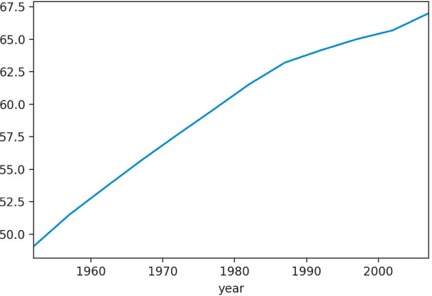
global_yearly_life_expectancy.plot()
1.6 Conclusion
This chapter explained how to load up a simple data set and start looking at specific observations. It may seem tedious at first to look at observations this way, especially if you are already familiar with the use of a spreadsheet program. Keep in mind that when doing data analytics, the goal is to produce reproducible results, and to not repeat repetitive tasks. Scripting languages give you that ability and flexibility.
Along the way you learned about some of the fundamental programming abilities and data structures that Python has to offer. You also encountered a quick way to obtain aggregated statistics and plots. The next chapter goes into more detail about the Pandas DataFrame and Series object, as well as other ways you can subset and visualize your data.
As you work your way though this book, if there is a concept or data structure that is foreign to you, check the various appendices for more information on that topic. Many fundamental programming features of Python are covered in the appendices.