
14. Model Diagnostics
14.1 Introduction
Building models is a continuous art. As we start adding and removing variables from our models, we need a means to compare models with one another and a consistent way of measuring model performance. There are many ways we can compare models, and this chapter describes some of these methods.
14.2 Residuals
The residuals of a model compare what the model calculates and the actual values in the data. Let’s fit some models on a housing data set.
import pandas as pd
housing = pd.read_csv('../data/housing_renamed.csv')
print(housing.head())
neighborhood type units year_built sq_ft income
0 FINANCIAL R9-CONDOMINIUM 42 1920.0 36500 1332615
1 FINANCIAL R4-CONDOMINIUM 78 1985.0 126420 6633257
2 FINANCIAL RR-CONDOMINIUM 500 NaN 554174 17310000
3 FINANCIAL R4-CONDOMINIUM 282 1930.0 249076 11776313
4 TRIBECA R4-CONDOMINIUM 239 1985.0 219495 10004582
income_per_sq_ft expense expense_per_sq_ft net_income
0 36.51 342005 9.37 990610
1 52.47 1762295 13.94 4870962
2 31.24 3543000 6.39 13767000
3 47.28 2784670 11.18 8991643
4 45.58 2783197 12.68 7221385
value value_per_sq_ft boro
0 7300000 200.00 Manhattan
1 30690000 242.76 Manhattan
2 90970000 164.15 Manhattan
3 67556006 271.23 Manhattan
4 54320996 247.48 Manhattan
We’ll begin with a multiple linear regression model with three covariates.
import statsmodels
import statsmodels.api as sm
import statsmodels.formula.api as smf
house1 = smf.glm('value_per_sq_ft ~ units + sq_ft + boro',
data=housing).fit()
print(house1.summary())
Generalized Linear Model Regression Results
==============================================================================
Dep. Variable: value_per_sq_ft No. Observations: 2626
Model: GLM Df Residuals: 2619
Model Family: Gaussian Df Model: 6
Link Function: identity Scale: 1879.49193485
Method: IRLS Log-Likelihood: -13621.
Date: Tue, 12 Sep 2017 Deviance: 4.9224e+06
Time: 05:07:05 Pearson chi2: 4.92e+06
No. Iterations: 2
=========================================================================================
coef std err z P>|z| [0.025 0.975]
-----------------------------------------------------------------------------------------
Intercept 43.2909 5.330 8.122 0.000 32.845 53.737
boro[T.Brooklyn] 34.5621 5.535 6.244 0.000 23.714 45.411
boro[T.Manhattan] 130.9924 5.385 24.327 0.000 120.439 141.546
boro[T.Queens] 32.9937 5.663 5.827 0.000 21.895 44.092
boro[T.Staten Island] -3.6303 9.993 -0.363 0.716 -23.216 15.956
units -0.1881 0.022 -8.511 0.000 -0.231 -0.145
sq_ft 0.0002 2.09e-05 10.079 0.000 0.000 0.000
=========================================================================================
/home/dchen/anaconda3/envs/book36/lib/python3.6/site-
packages/statsmodels/compat/pandas.py:56: FutureWarning: The
pandas.core.datetools module is deprecated and will be removed in a
future version. Please use the pandas.tseries module instead.
from pandas.core import datetools
We can plot the residuals of our model (Figure 14.1). What we are looking for is a plot with a random scattering of points. If a pattern is apparent, then we will need to investigate our data and model to see why this pattern emerged.
import seaborn as sns
import matplotlib.pyplot as plt
fig, ax = plt.subplots()
ax = sns.regplot(x=house1.fittedvalues,
y=house1.resid_deviance, fit_reg=False)
plt.show()
fig.savefig('p5-ch-model_diagnostics/figures/resid_1')
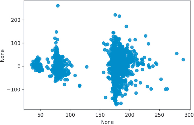
This residual plot is extremely concerning because it contains obvious clusters and groups. Let’s can color our plot by the boro variable, which indicates the borough of New York where the data apply (Figure 14.2).
res_df = pd.DataFrame({
'fittedvalues': house1.fittedvalues,
'resid_deviance': house1.resid_deviance,
'boro': housing['boro']
})
fig = sns.lmplot(x='fittedvalues', y='resid_deviance',
data=res_df, hue='boro', fit_reg=False)
plt.show()
fig.savefig('p5-ch-model_diagnostics/figures/resid_boros')
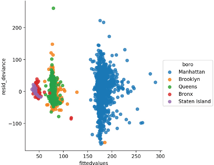
When we color our points based on boro, you can see that the clusters are highly governed by the value of this variable.
14.2.1 Q-Q Plots
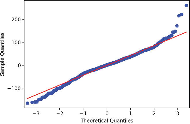
A q-q plot is a graphical technique that determines whether your data conforms to a reference distribution. Since many models assume the data is normally distributed, a q-q plot is one way to make sure your data really is normal (Figure 14.3).
from scipy import stats
resid = house1.resid_deviance.copy()
resid_std = stats.zscore(resid)
fig = statsmodels.graphics.gofplots.qqplot(resid, line='r')
plt.show()
fig.savefig('p5-ch-model_diagnostics/figures/house_1_qq')
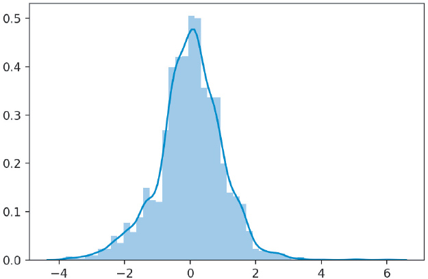
We can also plot a histogram of the residuals to see if our data is normal (Figure 14.4).
fig, ax = plt.subplots()
ax = sns.distplot(resid_std)
plt.show()
fig.savefig('p5-ch-model_diagnostics/figures/house1_resid_std')
If the points on the q-q plot lie on the red line, then that means our data match our reference distribution. If the points do not lie on this line, then one thing we can do is apply a transformation to our data. Table 14.1 shows which transformations can be performed on your data. If the q-q plot of points is convex compared to the red reference line, then you can transform your data toward the top of the table. If the q-q plot of points is concave compared to the red reference line, then you can transform your data toward the bottom of the table.
xp |
Equivalent |
Description |
x2 |
x2 |
Square |
x1 |
x |
|
|
|
Square root |
“x”x |
log(x) |
Log |
|
|
Reciprocal square root |
x–1 |
|
Reciprocal |
x–2 |
|
Reciprocal square |
14.3 Comparing Multiple Models
Now that we know how to assess a single model, we need a means to compare multiple models so that we can pick the “best” one.
14.3.1 Working With Linear Models
We begin by fitting five models. Note that some of the models use the + operator to add covariates to the model, whereas others use the * operator. To specify an interaction in our model, we use the * operator. That is, the variables that are interacting are behaving in a way that is not independent from one another, but rather in such a way that their values affect one another and are not simply additive.
# the original housing data set has a column named class
# this would cause an error if we used 'class'
# because 'class' is a Python keyword
# the column was renamed to 'type'
f1 = 'value_per_sq_ft ~ units + sq_ft + boro'
f2 = 'value_per_sq_ft ~ units * sq_ft + boro'
f3 = 'value_per_sq_ft ~ units + sq_ft * boro + type'
f4 = 'value_per_sq_ft ~ units + sq_ft * boro + sq_ft * type'
f5 = 'value_per_sq_ft ~ boro + type'
house1 = smf.ols(f1, data=housing).fit()
house2 = smf.ols(f2, data=housing).fit()
house3 = smf.ols(f3, data=housing).fit()
house4 = smf.ols(f4, data=housing).fit()
house5 = smf.ols(f5, data=housing).fit()
With all our models, we can collect all of our coefficients and the model with which they are associated.
mod_results = pd.concat([house1.params, house2.params, house3.params,
house4.params, house5.params], axis=1).
rename(columns=lambda x: 'house' + str(x + 1)).
reset_index().
rename(columns={'index': 'param'}).
melt(id_vars='param', var_name='model', value_name='estimate')
print(mod_results.head())
param model estimate
0 Intercept house1 43.290863
1 boro[T.Brooklyn] house1 34.562150
2 boro[T.Manhattan] house1 130.992363
3 boro[T.Queens] house1 32.993674
4 boro[T.Staten Island] house1 -3.630251
print(mod_results.tail())
param model estimate
85 type[T.R4-CONDOMINIUM] house5 20.457035
86 type[T.R9-CONDOMINIUM] house5 1.293322
87 type[T.RR-CONDOMINIUM] house5 -11.680515
88 units house5 NaN
89 units:sq_ft house5 NaN
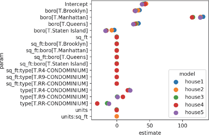
Since it’s not very useful to look at a large column of values, we can plot our coefficients to quickly see how the models are estimating parameters in relation to each other (Figure 14.5).
fig, ax = plt.subplots()
ax = sns.pointplot(x="estimate", y="param", hue="model",
data=mod_results,
dodge=True, # jitter the points
join=False) # don't connect the points
plt.tight_layout()
plt.show()
Now that we have our linear models, we can use the analysis of variance (ANOVA) method to compare them. The ANOVA will give us the residual sum of sqaures (RSS), which is one way we can measure performance (lower is better).
model_names = ['house1', 'house2', 'house3', 'house4', 'house5']
house_anova = statsmodels.stats.anova.anova_lm(
house1, house2, house3, house4, house5)
house_anova.index = model_names
print(house_anova)
df_resid ssr df_diff ss_diff F
house1 2619.0 4.922389e+06 0.0 NaN NaN
house2 2618.0 4.884872e+06 1.0 37517.437605 20.039049
house3 2612.0 4.619926e+06 6.0 264945.539994 23.585728
house4 2609.0 4.576671e+06 3.0 43255.441192 7.701289
house5 2618.0 4.901463e+06 -9.0 -324791.847907 19.275539
Pr(>F)
house1 NaN
house2 7.912333e-06
house3 2.754431e-27
house4 4.025581e-05
house5 NaN
/home/dchen/anaconda3/envs/book36/lib/python3.6/site-
packages/scipy/stats/_distn_infrastructure.py:879: RuntimeWarning:
invalid value encountered in greater
return (self.a < x) & (x < self.b)
/home/dchen/anaconda3/envs/book36/lib/python3.6/site-
packages/scipy/stats/_distn_infrastructure.py:879: RuntimeWarning:
invalid value encountered in less
return (self.a < x) & (x < self.b)
/home/dchen/anaconda3/envs/book36/lib/python3.6/site-
packages/scipy/stats/_distn_infrastructure.py:1818: RuntimeWarning:
invalid value encountered in less_equal
cond2 = cond0 & (x <= self.a)
Another way we can calculate model performance is by using the Akaike information criterion (AIC) and the Bayesian information criterion (BIC). These methods apply a penalty for each feature that is added to the model. Thus, we should strive to balance performance and parsimony (lower is better).
house_models = [house1, house2, house3, house4, house5]
house_aic = list(
map(statsmodels.regression.linear_model.RegressionResults.aic,
house_models))
house_bic = list(
map(statsmodels.regression.linear_model.RegressionResults.bic,
house_models))
# remember dicts are unordered
abic = pd.DataFrame({
'model': model_names,
'aic': house_aic,
'bic': house_bic
})
print(abic)
aic bic model
0 27256.031113 27297.143632 house1
1 27237.939618 27284.925354 house2
2 27103.502577 27185.727615 house3
3 27084.800043 27184.644733 house4
4 27246.843392 27293.829128 house5
14.3.2 Working With GLM Models
We can perform the same calculations and model diagnostics on generalized linear models (GLMs). However, the ANOVA is simply the deviance of the model.
def anova_deviance_table(*models):
return pd.DataFrame({
'df_residuals': [i.df_resid for i in models],
'resid_stddev': [i.deviance for i in models],
'df': [i.df_model for i in models],
'deviance': [i.deviance for i in models]
})
f1 = 'value_per_sq_ft ~ units + sq_ft + boro'
f2 = 'value_per_sq_ft ~ units * sq_ft + boro'
f3 = 'value_per_sq_ft ~ units + sq_ft * boro + type'
f4 = 'value_per_sq_ft ~ units + sq_ft * boro + sq_ft * type'
f5 = 'value_per_sq_ft ~ boro + type'
glm1 = smf.glm(f1, data=housing).fit()
glm2 = smf.glm(f2, data=housing).fit()
glm3 = smf.glm(f3, data=housing).fit()
glm4 = smf.glm(f4, data=housing).fit()
glm5 = smf.glm(f5, data=housing).fit()
glm_anova = anova_deviance_table(glm1, glm2, glm3, glm4, glm5)
print(glm_anova)
deviance df df_residuals resid_stddev
0 4.922389e+06 6 2619 4.922389e+06
1 4.884872e+06 7 2618 4.884872e+06
2 4.619926e+06 13 2612 4.619926e+06
3 4.576671e+06 16 2609 4.576671e+06
4 4.901463e+06 7 2618 4.901463e+06
We can do the same set of calculations in a logistic regression.
# create a binary variable
housing['high_value'] = (housing['value_per_sq_ft'] >= 150).
astype(int)
print(housing['high_value'].value_counts())
0 1619
1 1007
Name: high_value, dtype: int64
# create and fit our logistic regression using GLM
f1 = 'high_value ~ units + sq_ft + boro'
f2 = 'high_value ~ units * sq_ft + boro'
f3 = 'high_value ~ units + sq_ft * boro + type'
f4 = 'high_value ~ units + sq_ft * boro + sq_ft * type'
f5 = 'high_value ~ boro + type'
logistic = statsmodels.genmod.families.family.Binomial(
link=statsmodels.genmod.families.links.logit
)
glm1 = smf.glm(f1, data=housing, family=logistic).fit()
glm2 = smf.glm(f2, data=housing, family=logistic).fit()
glm3 = smf.glm(f3, data=housing, family=logistic).fit()
glm4 = smf.glm(f4, data=housing, family=logistic).fit()
glm5 = smf.glm(f5, data=housing, family=logistic).fit()
# show the deviances from our GLM models
print(anova_deviance_table(glm1, glm2, glm3, glm4, glm5))
deviance df df_residuals resid_stddev
0 1695.631547 6 2619 1695.631547
1 1686.126740 7 2618 1686.126740
2 1636.492830 13 2612 1636.492830
3 1619.431515 16 2609 1619.431515
4 1666.615696 7 2618 1666.615696
Finally, we can create a table of AIC and BIC values.
mods = [glm1, glm2, glm3, glm4, glm5]
mods_aic = list(
map(statsmodels.regression.linear_model.RegressionResults.aic,
mods))
mods_bic = list(
map(statsmodels.regression.linear_model.RegressionResults.bic,
mods))
# remember dicts are unordered
abic = pd.DataFrame({
'model': model_names,
'aic': house_aic,
'bic': house_bic
})
print(abic)
aic bic model
0 27256.031113 27297.143632 house1
1 27237.939618 27284.925354 house2
2 27103.502577 27185.727615 house3
3 27084.800043 27184.644733 house4
4 27246.843392 27293.829128 house5
Looking at all these measures, we can say Model 4 is performing the best so far.
14.4 k-Fold Cross-Validation
Cross-validation is another technique to compare models. One of the main benefits is that it can account for how well your model performs on new data. It does this by partitioning your data into k parts. It holds one of the parts aside as the “test” set and then fits the model on the remaining k – 1 parts, the “training” set. The fitted model is then used on the “test” and an error rate is calculated. This process is repeated until all k parts have been used as a “test” set. The final error of the model is some average across all the models.
Cross-validation can be performed in many different ways. The method just described is called “k-fold cross-validation.” Alternative ways of performing cross-validation include “leave-one-out cross-validation,” in which the training data consists of all the data except one observation designated as the test set.
Here we will split our data into k – 1 testing and training data sets.
from sklearn.model_selection import train_test_split
from sklearn.linear_model import LinearRegression
print(housing.columns)
Index(['neighborhood', 'type', 'units', 'year_built', 'sq_ft',
'income', 'income_per_sq_ft', 'expense', 'expense_per_sq_ft',
'net_income', 'value', 'value_per_sq_ft', 'boro',
'high_value'],
dtype='object')
# get training and test data
X_train, X_test, y_train, y_test = train_test_split(
pd.get_dummies(housing[['units', 'sq_ft', 'boro']],
drop_first=True),
housing['value_per_sq_ft'],
test_size=0.20,
random_state=42
)
We can get a score that indicates how well our model is performing using our test data.
lr = LinearRegression().fit(X_train, y_train)
print(lr.score(X_test, y_test))
0.613712528503
Since sklearn relies heavily on the numpy ndarray, the patsy library allows you to specify a formula just like the formula API in statsmodels, and it returns a proper numpy array you can use in sklearn.
Here is the same code as before, but using the dmatrices function in the patsy library.
from patsy import dmatrices
y, X = dmatrices('value_per_sq_ft ~ units + sq_ft + boro', housing, return_type="dataframe")
X_train, X_test, y_train, y_test = train_test_split(
X, y, test_size=0.20, random_state=42)
lr = LinearRegression().fit(X_train, y_train)
print(lr.score(X_test, y_test))
0.613712528503
To perform a k-fold cross-validation, we need to import this function from sklearn.
from sklearn.model_selection import KFold, cross_val_score
# get a fresh new housing data set
housing = pd.read_csv('../data/housing_renamed.csv')
We now have to specify how many folds we want. This number depends on how many rows of data you have. If your data does not include too many observations, you may opt to select a smaller k (e.g., 2). Otherwise, a k between 5 to 10 is fairly common. However, keep in mind that the trade-off with higher k values is more computation time.
kf = KFold(n_splits=5)
y, X = dmatrices('value_per_sq_ft ~ units + sq_ft + boro', housing)
Next we can train and test our model on each fold.
coefs = []
scores = []
for train, test in kf.split(X):
X_train, X_test = X[train], X[test] y_train,
y_test = y[train], y[test]
lr = LinearRegression().fit(X_train, y_train)
coefs.append(pd.DataFrame(lr.coef_))
scores.append(lr.score(X_test, y_test))
We can also view the results.
coefs_df = pd.concat(coefs)
coefs_df.columns = X.design_info.column_names
coefs_df
Intercept boro[T.Brooklyn] boro[T.Manhattan] boro[T.Queens]
0 0.0 33.369037 129.904011 32.103100
0 0.0 32.889925 116.957385 31.295956
0 0.0 30.975560 141.859327 32.043449
0 0.0 41.449196 130.779013 33.050968
0 0.0 -38.511915 56.069855 -17.557939
boro[T.Staten Island] units sq_ft
0 -4.381085 -0.205890 0.000220
0 -4.919232 -0.146180 0.000155
0 -4.379916 -0.179671 0.000194
0 -3.430209 -0.207904 0.000232
0 0.000000 -0.145829 0.000202
We can take a look at the average coefficient across all folds using apply and the np.mean function.
import numpy as np
print(coefs_df.apply(np.mean))
Intercept 0.000000
boro[T.Brooklyn] 20.034361
boro[T.Manhattan] 115.113918
boro[T.Queens] 22.187107
boro[T.Staten Island] -3.422088
units -0.177095
sq_ft 0.000201
dtype: float64
We can also look at our scores. Each model has a default scoring method.
LinearRegression, for example, uses the R2 (coefficient of determination) regression score function.1
1. sklearn R2 scoring: http://scikit-learn.org/stable/modules/generated/sklearn.metrics.r2_score.html
print(scores)
[0.027314162906420303, -0.55383622124079213, -0.15636371688048567,
-0.32342020619288148, -1.6929655586930985]
We can also use cross_val_scores (for cross-validation scores) to calculate our scores.
# use cross_val_scores to calculate CV scores
model = LinearRegression()
scores = cross_val_score(model, X, y, cv=5)
print(scores)
[ 0.02731416 -0.55383622 -0.15636372 -0.32342021 -1.69296556]
If we were to compare multiple models with each other, we would compare the average of the scores.
print(scores.mean())
-0.53985430802
Now we’ll refit all our models using k-fold cross-validation.
# create the predictor and response matrices
y1, X1 = dmatrices('value_per_sq_ft ~ units + sq_ft + boro',
housing)
y2, X2 = dmatrices('value_per_sq_ft ~ units*sq_ft + boro',
housing)
y3, X3 = dmatrices('value_per_sq_ft ~ units + sq_ft*boro + type',
housing)
y4, X4 = dmatrices('value_per_sq_ft ~ units + sq_ft*boro + sq_ft*type',
housing)
y5, X5 = dmatrices('value_per_sq_ft ~ boro + type', housing)
# fit our models
model = LinearRegression()
scores1 = cross_val_score(model, X1, y1, cv=5)
scores2 = cross_val_score(model, X2, y2, cv=5)
scores3 = cross_val_score(model, X3, y3, cv=5)
scores4 = cross_val_score(model, X4, y4, cv=5)
scores5 = cross_val_score(model, X5, y5, cv=5)
We can now look at our cross-validation scores.
scores_df = pd.DataFrame([scores1, scores2, scores3,
scores4, scores5])
print(scores_df.apply(np.mean, axis=1))
0 -5.398543e-01
1 -1.088184e+00
2 -3.569632e+26
3 -1.141180e+27
4 -3.227148e+25
dtype: float64
Once again, we see that Model 4 has the best performance.
14.5 Conclusion
When we are working with models, it’s important to measure their performance. Using ANOVA for linear models, looking at deviance for GLM models, and using cross-validation are all ways we can measure error and performance when trying to pick the best model.